Signs of Phase Transitions in Two-Nucleon Systems

Abstract

The properties of dense nuclear matter under extreme conditions are a subject of the large experimental activities worldwide. Heavy-ion collision experiments are the agenda item at RHIC, LHC, FAIR, and NICA facilities. Meanwhile, a complementary approach to the heavy-ion collision researches devoted to investigation of phase transitions in few-nucleon systems has not been discussed. In this paper, we try to fill up the gap. It is shown that signals of the phase transition of deuteron into 6-q bag as well as signs of formation of the pion Bose-Einstein condensate in compressed two-nucleon systems might be already observed in deuteron-deuteron collisions.

I Introduction

High-energy nuclear collisions allow the study of new phases of nuclear matter under extreme conditions at which the phase transition of nuclear matter to a color-deconfined state was predicted by the fundamental theory of strong interactions, the Quantum Chromodynamics (QCD). The experimental programs at BNL and CERN have already confirmed that the extreme conditions of matter necessary to reach the new phase can be reached in the high-energy nuclear collisions. However, identifying and studying the properties of those phases is a challenging task, mainly because of many-body effects and nonperturbative nature of the processes involved. These challenges stimulate putting forward new experimental and theoretical ideas aimed at search of unambiguous signatures of the phase transition onset. Recently a proposal of QCD investigation at high density and low temperature complementary to the high-energy heavy nuclear collisions was suggested Kostenko1 ; Kostenko2 . The proposal is based on the fact that a large number of nucleons in the interaction region is not necessary for the phase transition to occur, and only a change of the vacuum state should be initiated by some experimental environment. Detection of two- and three-nucleon short range correlations CLAS affords an opportunity to use the dense few-nucleon correlated systems of this type (SRC) as targets which correspond to small fragments of nuclear matter in the dynamically broken chiral symmetry states. Collisions of SRC with bombarding particles can initiate the chiral phase transition, ending in the creation of a multi-baryon(MB). Thus, the observation of MB would be a direct evidence of the chiral condensate disappearance and the chiral symmetry restoration in the interaction area. Separation of a MB mass from the secondary particle background is feasible if the MB decay width is narrow enough. That requires the excitation energy of produced MB to be low. For this purpose, it is reasonable to select only those experimental events in which the MB creation is accompanied with a high momentum particle, taking away an essential part of the energy from the interaction region (a cooling effect). In this paper, we focus on new developments in this direction outlined in Kostenko1 ; Kostenko2 and put them in a context with some of older experimental data taken at JINR synchrophasotron Baldin ; Troyan1 ; Troyan2 ; Troyan3 .

An experiment Baldin was designed for measurement of the cross-sections of elastic pp-, ND-, and DD-scattering at 8.9 GeV momentum of primary protons and deuterons. Particularly, three peaks were observed in the spectrum of the missing masses of the reaction D$+$D$\to$M${}_{X}+$D at $t=-0.495$ GeV² (see Fig. 1).

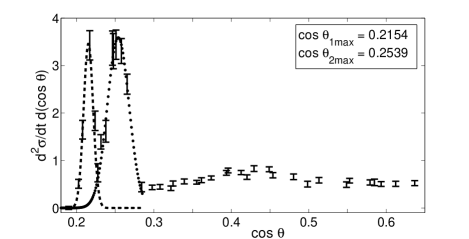
Figure 1: Double differential cross-sections, in mb$\cdot$c²/GeV², of the D$+$D$\to$M${}_{X}+$D reaction against cosine of the target nucleus scattering angle Baldin . The dashed and dotted curves correspond to approximations of the first two peaks by the Gaussian functions which maxima positions are given in the insertion.

Till now the first of them corresponding to the most heavy M_X was estimated to cover the elastic DD scattering; the second one was interpreted as a manifestation of the scattering of a projectile deuteron’s nucleon by the target deuteron; in regard to the third peak, it was suggested to appear because of 1) a contribution of the constituent quark scattering, 2) a contribution of an excited state of deuteron (e.g., 6q-bag), and 3) to be a kinematic manifestation of a baryon N^∗ with a value of mass in the neighborhood of 1400 MeV.

Experimental findings occurred after the paper Baldin was written give cause for re-examination of its conclusions. Data from Troyan1 ; Troyan2 employing 38915 events will play an especially important role in our consideration. So far as the interpretations of the third peak promise detection of the chiral phase transition, we begin with it. Thereafter problems concerning the first two peaks will be discussed.

II Possible dibaryons in the third peak region

Figure 2: The experimental data (dots) in the range of the third peak and their explanation by the sum of contributions of N$+$D$\to$X$+$D reactions (dashed line). The top scale corresponds to the kinematics of reaction D$+$D$\to$X$+$D which implies the dibaryon production. A possible contribution of a dibaryon at 2.37 GeV, $\Gamma\approx$ 70 MeV, reported by WASA-at-COSY Collaboration WASA into the third region is shown with the overturned solid line.

Kinematics of the N$+$D$\to$X$+$D reaction reads

$${{\it M_{X}}}^{2}={{\it M_{N}}}^{2}+t+$$ (1)

$$+1/2\,{\frac{\sqrt{{{\it P_{1}}}^{2}+4\,{{\it M_{N}}}^{2}}t+{\it P_{1}}\,\sqrt{t\left(-4\,{{\it M_{D}}}^{2}+t\right)}\cos\theta}{{\it M_{D}}}},$$

where $P_{1}$ is momentum of the primary deuteron, $P_{1}=8.9$, and $M_{N}=0.94$, $M_{D}=1.8756$ GeV. Here X may be any baryon resonance or nucleon escorted by one or more pions. In framework of this model, the differential cross-section $d^{2}\sigma/dtdM_{X}^{2}$ in a region $M_{X}\approx 1.4$ GeV may be expressed as follows:

$$C_{0}+\sum\limits_{i=1}^{3}{C_{i}f_{i}}+2\sum\limits_{\begin{array}[]{*{20}c}{i,j=1}\\ {i<j}\\ \end{array}}^{3}{k_{ij}\sqrt{C_{i}C_{j}f_{i}f_{i}}\cos(\varphi_{i}-}\varphi_{j}),$$ (2)

where resonances N(1440), N(1520), and N(1535) were taken into account. We have chosen functions $f_{i}$ in the formPilk $f_{i}=M_{i}\Gamma_{i}/((M_{X}^{2}-M_{i}^{2})^{2}+\Gamma_{i}^{2}M_{i}^{2})$. Data on baryon resonances were taken from ref. PDG ; a contribution of the reaction with nucleon and several pions in the final state was approximated by a constant; values of parameters in (2) were found to obtain the best description of the data, according to a global optimization procedure. We have introduced for the interference terms factors $k_{ij}\in[0,1]$ which take into account a value of indistinguishability of two different resonances. In Fig. 2, an attempt to explain a fine structure in the range of the third peak by the sum of contributions of reactions N$+$D$\to$X$+$D. One can see that, in principle, it possible to explain at least a part of the fine structure in the third peak region by the sum of contributions of the processes with nucleon excitations.

For the dibaryon production in the reaction D$+$D$\to$2B$+$D, the isospin conservation leads to $I_{2B}=0$. The kinematics,

$$M_{X}^{2}=M_{D}^{2}+t+\frac{{E_{1}t+P_{1}\sqrt{t(-4M_{D}^{2}+t)}\cos\theta}}{{M_{D}}},$$ (3)

states that the fine structure in the third peak region is described if one supposes the existence of a dibaryon at $M_{2B}\approx$ 2.38 GeV (see the upper scale in Fig. 2). It looks like it was recently reportedWASA by WASA-at-COSY Collaboration in reaction pp $\to$ D $\pi^{0}\pi^{0}$ at 2.37 GeV, $\Gamma\approx$ 70 MeV. Similar masses were found in a pp$\pi^{+}$ system in Troyan3 . Therefore, it is plausible to expect that these hypothetic dibaryons decay into two nucleons and one or two pions.

It is interesting to check if the fine structure in the third peak region may be explained as constituent quark scattering in reaction qD$\to$qD. The elastic scattering of a constituent quark by the target deuteron may be considered in the framework of a model in which values of momentum and mass of the projectile quark are considered in the form

$$P_{q}=xP_{1},\qquad M_{q}=xM_{D},$$

where $x$ is determined from kinematics of the reaction. The model gives for $\cos\theta=0.396$ corresponding to $M_{2B}\approx$ 2.38 GeV, a value of quark mass

$$M_{q}=\frac{{-M_{D}^{2}t}}{{E_{1}t+P_{1}\sqrt{t(-4M_{D}^{2}+t)}\cos\theta}},$$

about 0.351 GeV. It contradicts to modern constituent quark models; see, e.g., ref. Jovan in which $M_{q}=0.318$ GeV.

III The first two peaks’ puzzle

The Gaussian two-peak approximation results in $\cos\theta_{1}=0.2154$ and $\cos\theta_{2}=0.2539$ for the location of the first two peaks’ maxima (see Fig. 1). It was very unexpected to find that elastic D-D scattering gives the angle distribution with a maximum at 0.2272, see (3) for $M_{X}=M_{D}$, i.e. between $\cos\theta_{1}$ and $\cos\theta_{2}$. Similarly, elastic N-D scattering described by (1) with $M_{X}=M_{N}$ has a maximum at 0.2661, clearly shifted from the second peak location. Thus, the explanation of the first two peaks by means of contributions of the elastic D-D and N-D scattering fails and their origin remains unclear. At first glance, the discrepancy may be attributed to systematic errors committed in the experiment, but a subsequent calculations found out that another astonishing explanation is more plausible.

To explain positions of the first two peaks, different models have been tried out. The models were based on the fact that only the recoil deuteron was unambiguously identified inBaldin but masses of all other participants were unknown. Therefore, any transitions X$+$Y$\to$Z$+$D are allowed to be taken into account. For example, a scattering X$+$D $\to$ D$+$D explains the first peak location if one assigns to X a value of mass of about 1913 Mev which turns out to be close to 1916$\pm$2 MeV, observed in a pp dibaryon spectrum by Yu.A. Troyan Troyan1 ; Troyan2 . A model D$+$D $\to$ X$+$D gives for the second peak location if one assumes $M_{X}=1965$ MeV. The data from Troyan1 ; Troyan2 contain a corresponding dibaryon with $M_{X}=1965\;\pm 2$ MeV.

Analysis of other models showed that almost each dibaryon observed in Troyan1 ; Troyan2 can give a contribution to the first two peaks observed in Baldin , under an assumption that masses of dibaryons detected in the np-system are 1 MeV less than the corresponding masses in the pp-system. In Table 1, considered reactions are shown in the first column. The second column specifies masses of ingoing or outgoing objects in the deuteron scattering experiment Baldin . Dibaryon masses found for the pp-system in refs. Troyan1 ; Troyan2 are given in the third column.

Table 1: Kinematically admissible masses (KAM) which might contribute to the first or second peak in the experiment Baldin . Proton-proton dibaryon masses are taken from Troyan1 ; Troyan2 .

Reaction	KAM	pp-dibaryon masses Troyan1 ; Troyan2
X$+$D$\to$D+D	1913	1916$\pm$2
D$+$X$\to$D+D	1884	1886$\pm$1
D$+$X$\to$X+D	1886	1886$\pm$1
X$+$X$\to$X+D	1884	1886$\pm$1
X$+$X$\to$Y+D	1886$\to$1898	1886$\pm$1, 1898$\pm$1
X$+$D$\to$Y+D	1916$\to$1884	1916$\pm$2, 1886$\pm$1
	1965$\to$1937	1965$\pm$2, 1937$\pm$2
	1980$\to$1953	1980$\pm$2, 1955$\pm$2
	2106$\to$2086	2106$\pm$2, 2087$\pm$3
D$+$D$\to$X+D	1965	1965$\pm$2
X$+$D$\to$Y+D	1886$\to$1966	1886$\pm$1, 1965$\pm$2
	1898$\to$1979	1898$\pm$1, 1980$\pm$2
	1916$\to$1998	1916$\pm$2, 1999$\pm$2
	1937$\to$2020	1937$\pm$2, 2017$\pm$3
	1999$\to$2086	1999$\pm$2, 2087$\pm$3
	2017$\to$2105	2017$\pm$3, 2106$\pm$3

The reactions above the horizontal line explain the first peak and the reactions below it explain the second one. It is possible to verify that the reactions considered for explanation of the data Baldin reproduce masses of all dibaryons observed in refs. Troyan1 ; Troyan2 , with the exception of two of them at 2008$\pm$3 and 2046$\pm$3 MeV/c².

IV An equidistant spectrum assumption

With an assumption that some of dibaryons were unrecognized in the experiments Troyan1 ; Troyan2 , it is possible to approximate the pp-dibaryon mass spectrum within rather small, at 1 – 2 MeV/c² level, experimental errors by the formula

$$M_{n}=M_{NN}+10.08\;n,$$ (4)

where $n=0,1,2,...,40$, all values are taken in MeV, $M_{NN}$ is equal to the value of mass of two protons. A quality of this assumption is seen, e.g., from a fact that only 4 dibaryons might be unrecognized in Troyan1 ; Troyan2 among the first 14 ones predicted by (4).

To check the suggestion of the similarity of pp- and np-dibaryon mass spectrum, which follows from TABLE 1, we accepted the relation (4) for np-dibaryons too, only changing $M_{NN}$ with the deuteron value of mass. In Tables 2 and 3, the second column specifies masses of ingoing or outgoing particles, which are allowed by kinematics,

$$M_{Y}^{2}=M_{X}^{2}+t+M_{X}P_{1}\frac{{\sqrt{t(-4M_{d}^{2}+t)}}}{{M_{d}^{2}}}\cos\theta+\frac{{M_{X}E_{1}t}}{{M_{d}^{2}}},$$

of the X$+$D$\to$Y+D reaction. Dibaryon masses for the np-system computed according to (4) are shown in the third column.

One can see that each of dibaryons predicted by (4) in the range from 1886 to 2198 may contribute to the first or second peaks, observed in ref. Baldin . Thus, new dibaryons predicted by the equidistant spectrum (4), taken as an assumption on basis of Troyan1 ; Troyan2 , are also confirmed by the data Baldin . Moreover, quality of the description definitely improves, since no dibaryon mass calculated using (4) is now lost in the description of the data from Baldin .

Table 2: Kinematically admissible masses (KAM) which might contribute to the first peak in X$+$D$\to$Y+D reaction. Dibaryon masses are taken according to the equidistant spectrum assumption.

Reaction	KAM	dibaryon masses, (4)
X$+$D$\to$Y+D	1916$\to$1884	1916, 1886
	1926$\to$1895	1926, 1896
	1936$\to$1905	1936, 1906
	1946$\to$1916	1946, 1916
	1956$\to$1927	1956, 1926
	1966$\to$1938	1966, 1936
	1976$\to$1948	1976, 1946
	1986$\to$1959	1986, 1956
	2047$\to$2024	2047, 2027
	2057$\to$2034	2057, 2037
	2067$\to$2045	2067, 2047
	2077$\to$2056	2077, 2057
	2087$\to$2066	2087, 2067
	2097$\to$2078	2097, 2077
	2107$\to$2087	2107, 2087
	2118$\to$2099	2118, 2097
	2128$\to$2109	2128, 2107
	2138$\to$2120	2138, 2118
	2148$\to$2131	2148, 2128
	2158$\to$2141	2158, 2138

Table 3: Kinematically admissible masses (KAM), which might contribute to the second peak in X$+$D$\to$Y+D reaction. Dibaryon masses are taken according to the equidistant spectrum assumption.

Reaction	KAM	dibaryon masses, (4)
X$+$D$\to$Y+D	1886$\to$1966	1886, 1966
	1896$\to$1977	1896, 1976
	1916$\to$1998	1916, 1997
	1926$\to$2009	1926, 2007
	1936$\to$2019	1936, 2017
	1946$\to$2030	1946, 2027
	1997$\to$2084	1997, 2087
	2007$\to$2095	2007, 2097
	2017$\to$2105	2017, 2107
	2027$\to$2116	2027, 2118
	2037$\to$2127	2037, 2128
	2047$\to$2137	2047, 2138
	2057$\to$2148	2057, 2148
	2067$\to$2158	2067, 2158
	2077$\to$2169	2077, 2168
	2087$\to$2179	2087, 2178
	2097$\to$2190	2097, 2188
	2107$\to$2200	2107, 2198

V The dynamical Casimir effect

The equidistant spectrum regularity observed in Baldin ; Troyan1 ; Troyan2 hardly can be interpreted in the frame of the 6-q bag model which predicts a different form of spectrum. One may try to assign it to some kind of oscillator consisting of quarks coupled by gluon strings Wang . However, consideration of the oscillator wave function with the constituent quark mass value indicates that the oscillator should have enormous dimensions. For example, the state $\psi_{20}(x)$, lying in the middle of the spectrum observed inTroyan1 ; Troyan2 , has the length of about 50 fm.

Actually, it was difficult to find an explanation better than to associate the spectrum with the production of pion pairs, strongly bound to compressed nucleon matter by a deep potential $-U_{0}$. The parity conservation requires pions to be produced in pairs (see below). Therefore, a value of energy of a single pion

$$E=\sqrt{p^{2}+m^{2}-U_{0}}$$ (5)

should be equal to 5.04 MeV $\equiv{\rm E}_{\pi}$.

A meson field in a rectangular potential well, $\varphi(\vec{r},t)=e^{-iEt}\varphi_{E}(\vec{r})$, is described by the Klein - Gordon - Fock (KGF) steady-state equation,

$$\frac{1}{{r^{2}}}\frac{d}{{dr}}r^{2}\frac{{d\varphi_{E}(r)}}{{dr}}+(E^{2}-m^{2}+U_{0}))\varphi_{E}(r)=0$$

which has a solution $\varphi_{E}(r)=A\sin pr/r$ inside the well, and $\varphi_{E}(r)=Be^{-qr}/r$, $q=\sqrt{m^{2}-E^{2}}$ outside it. The requirement of continuity of the logarithmic derivative at the edge of the well, $r=a$, leads to a transcendental equation

$$p\;{\rm{ctg}}(pa)=\sqrt{m^{2}-E^{2}}$$ (6)

which is suitable for an estimation of relevant physical values in the interaction region. Spatial dimensions, corresponding to a given value of momentum transfer, is Halzen

$$a=\left\langle{r^{2}}\right\rangle^{1/2}\approx\sqrt{6}/{\rm{}}\left|{\vec{q}}\right|=0.68\;{\rm{fm}},\qquad\left|{\vec{q}}\right|^{2}=-t.$$

Solving eq. (6) with this value of $a$, one obtains $p\approx{\rm{0}}{\rm{.53\;GeV}},$ and using (5), one finds $\sqrt{U_{0}}\approx 0.55{\rm{\;GeV}}.$

Touching dynamics of the bound pion production, we suggest that it is induced by a change of a position of walls forming the potential well, in close analogy with emission of electromagnetic waves due to a motion of resonator s walls. This movement is capable to give energy to the virtual pions surrounding nucleons and turn them into real particles, the bound pions. Such a mechanism is known as the dynamical Casimir effect, firstly described in Fulling . It is closely connected with the Hawking radiation phenomenon and the Fulling-Unruh effect Birrell . The appeal of this model is it predicts the meson field with the vacuum quantum numbers, since the mesons are produced from the vacuum state due to the strong interaction, conserving all of them. Because of this, the pion field may be present at the ground state of deuteron, as it follows from the experimental dataBaldin , without breaking the deuteron quantum numbers. As far as the vacuum state has positive parity and the intrinsic parity of pion is negative, only even number of pions may be created in the process. Similarly, isospin conservation leads to a conclusion that pions may be produced in pairs with $I=0$, i.e. in the following vector of state:

$$\Psi_{2\pi}=\frac{1}{{\sqrt{3}}}(\pi_{a}^{+}\pi_{b}^{-}+\pi_{a}^{-}\pi_{b}^{+}-\pi_{a}^{0}\pi_{b}^{0}).$$

A picture of the pion production may be depicted as follows. At some instant $t_{1}$ a potential well capable to hold a bound pion energy level of a value $\varepsilon$ is formed. Then, rather quickly, the energy level ${\rm E}_{\pi}>\varepsilon$ is developed due to a shrinkage of the potential well in the nucleon collision process. After that at moment $t_{2}$, when nucleons is moving away, the energy level returns to the value $\varepsilon$, and afterwards it changes again to the Yukawa vacuum, corresponding $E=0$ and $q=m$. From mathematical viewpoint, creation of bound pions in this framework is totally equivalent to the parametric excitation of the quantum oscillator which appears after the quantization of the field.

VI Pion Bose-Einstein condensate

The time dependent KGF equation,

$$\left[{\frac{{\partial^{2}}}{{\partial t^{2}}}-\frac{{\partial^{2}}}{{\partial r^{2}}}+m^{2}-U_{0}}\right]\psi(r,t)=0,$$ (7)

with the evolving boundary conditions gives the wave function inside the well,

$$\varphi(r,t)=\chi(t)\sin pr/r,$$

where $\chi(t)$ describes an increasing amplitude of the field which manifests itself in the pion production. It obeys the equation

$$\frac{{\partial^{2}\chi(t)}}{{\partial t^{2}}}+(p^{2}+m^{2}-U_{0})\chi(t)=0$$ (8)

which has the same form as one for a classical oscillator with the varying frequency $\omega(t)=E(t)$. Therefore, it is possible to introduce the oscillator Hamiltonian

$$H=\frac{1}{2}\left({\pi_{\omega}^{2}+\omega^{2}(t)\chi_{\omega}^{2}}\right)=\omega(t)\left({a_{\omega}^{+}(t)a_{\omega}(t)+\frac{1}{2}}\right),$$ (9)

and draw eq. (8) in the Hamiltonian formalism framework:

$$\frac{{\partial H}}{{\partial\pi_{\omega}}}=\dot{\chi}_{\omega},\qquad-\frac{{\partial H}}{{\partial\chi_{\omega}}}=\dot{\pi}_{\omega},$$

where

$$\chi_{\omega}=\frac{{a_{\omega}+a_{\omega}^{+}}}{{\sqrt{2\omega}}},\qquad\pi_{\omega}=\frac{{a_{\omega}-a_{\omega}^{+}}}{{\sqrt{2\omega}}}.$$

The quantization may be performed by analogy with the similar procedure for a quantum field in the box via replacing functions $a_{\omega}(t)$ and $a_{\omega}^{+}(t)$ by the corresponding operators. The only non-essential difference is that now the field does not vanish at the boundary, but terminates in an exponentially decaying tail outside the potential well. Fields of this type are met in solid-state physics Shockley . Thus, the quantized field in the Heisenberg picture is written as

$$\hat{\varphi}(r,t)=\hat{\chi}_{\omega}(t)\sin pr/r=\left({\frac{{\hat{a}_{\omega}^{{\dagger}}(t)+\hat{a}_{\omega}(t)}}{{\sqrt{2\omega_{1}}}}}\right)\sin pr/r,$$

for any $t$ in the range of the pion production, $t_{1}\leq t\leq t_{2}$. Here $\omega_{1}=\omega(t_{1})=\varepsilon$. The time evolution of the field may be expressed in an equivalent form, using Bogoliubov’s canonical transformation (BCT):

$$\left({\begin{array}[]{*{20}c}{\hat{a}(\Delta t)}\\ {\hat{a}^{+}(\Delta t)}\\ \end{array}}\right)=\overbrace{\left({\begin{array}[]{*{20}c}{u(\Delta t)}&{v(\Delta t)}\\ {u^{*}(\Delta t)}&{v^{*}(\Delta t)}\\ \end{array}}\right)}^{S(\Delta t)}\left({\begin{array}[]{*{20}c}{\hat{a}_{S}}\\ {\hat{a}_{S}^{+}}\\ \end{array}}\right),$$ (10)

where $\hat{a}_{S}$, $\hat{a}_{S}^{+}$ are the annihilation and production operators in the Schrödinger representation, $u(\Delta t)$ and $v(\Delta t)$ are usual (non-operator) functions. It is obvious that matrices $S(\Delta t)$ generate a group under multiplication,

$$S(\Delta t)\equiv S(\Delta t_{1}+...+\Delta t_{n})=S(\Delta t_{n})...S(\Delta t_{1}).$$

The commutation relation requirement $[\hat{a}(t),\hat{a}^{+}(t)]=1$ leads to a constraint

$$\left|u(t)\right|^{2}-\left|v(t)\right|^{2}=1$$ (11)

which means that the group of dynamical symmetry is $SU(1,1).$

Now we turn to the Schrödinger picture and define the group action in the space of state vectors, rather than in a space of the parameters describing evolution of operators. Lie algebra of $SU(1,1)$ is defined by the commutation relations

$$\left[{\hat{K}_{1},\hat{K}_{2}}\right]=-i\hat{K}_{0},\;\;\left[{\hat{K}_{2},\hat{K}_{0}}\right]=i\hat{K}_{1},\;\;\left[{\hat{K}_{0},\hat{K}_{1}}\right]=i\hat{K}_{2},$$

or, after introducing

$$\hat{K}_{\pm}=\pm i(\hat{K}_{1}\pm i\hat{K}_{2}),$$

by

$$\left[{\hat{K}_{0},\hat{K}_{\pm}}\right]=\pm\hat{K}_{\pm},\qquad\left[{\hat{K}_{-},\hat{K}_{+}}\right]=2\hat{K}_{0}.$$

One can express elements of the $SU(1,1)$ group through its generators:

$$\hat{S}(dt)=e^{(\beta\hat{K}_{+}-\beta^{*}\hat{K}_{-}-i\gamma\hat{K}_{0})dt}.$$

But in the case of the Hamiltonian evolution

$$\hat{S}(dt)=e^{-i\hat{H}dt},$$

so that it is possible to rewrite Hamiltonian (9) in the form

$$\hat{H}=i(\beta\hat{K}_{+}-\beta^{*}\hat{K}_{-}-i\gamma\hat{K}_{0}).$$

Corresponding expressions for $\hat{K}_{+}$, $\hat{K}_{-}$ and $\hat{K}_{0}$ are

$$\hat{K}_{+}=\frac{{(\hat{a}^{{\dagger}})^{2}}}{2},\;\;\hat{K}_{-}=\frac{{\hat{a}^{2}}}{2},\;\;\hat{K}_{0}=\frac{{\hat{a}\hat{a}^{{\dagger}}+\hat{a}^{{\dagger}}\hat{a}}}{4}$$

for $\pi^{0}\pi^{0}$ and

$$\hat{K}_{+}=\hat{a}_{+}^{{\dagger}}\hat{a}_{-}^{{\dagger}},\;\hat{K}_{-}=\hat{a}_{+}\hat{a}_{-,}\;\hat{K}_{0}=\frac{1}{2}(\hat{a}_{+}^{{\dagger}}\hat{a}_{+}+\hat{a}_{-}^{{\dagger}}\hat{a}_{-}+1)$$

for $\pi^{+}\pi^{-}$. In fact, the operators $\hat{K}_{0}$ do not lead to a change of a particle number and it is possible to omit them, at least for particle number distribution calculations. Thus, the evolution operator may be defined as an element of the $SU(1,1)$ group of a kind $\hat{S}(t)=\exp{(\xi\hat{K}_{+}-\xi^{*}\hat{K}_{-})}.$ Therefore, the state of system at moment $t$ is estimated as

$$\left|{\psi_{t}}\right\rangle=\exp{(\xi\hat{K}_{+}-\xi^{*}\hat{K}_{-})}\left|0\right\rangle.$$ (12)

It is possible to notice a similarity of this state to the Glauber coherent state Glaub

$$\left|{\psi_{G}}\right\rangle=e^{\alpha a^{{\dagger}}-\alpha^{*}a}\left|0\right\rangle=e^{-\left|\alpha\right|^{2}/2}\sum\limits_{n=0}^{\infty}{\frac{{\alpha^{n}}}{{\sqrt{n!}}}}\left|n\right\rangle$$

which leads to the Poisson distribution for the probability to find $n$ particles in the $\left|{\psi_{G}}\right\rangle$ state,

$$w_{n}=\left|{\left\langle{n}\mathrel{\left|{\vphantom{n{\psi_{G}}}}\right.\kern-1.2pt}{{\psi_{G}}}\right\rangle}\right|^{2}=e^{-\left|\alpha\right|^{2}}\frac{{\left|\alpha\right|^{2n}}}{{n!}},{\rm{}}\left\langle n\right\rangle=\left|\alpha\right|^{2}.$$

Similarly, the state $\left|{\psi_{t}}\right\rangle$ readsPerel

$$\left|{\psi_{t}}\right\rangle=(1-\left|\eta\right|^{2})^{k}\sum\limits_{m=0}^{\infty}{\left({\frac{{\Gamma(m+2k)}}{{m!\Gamma(2k)}}}\right)^{1/2}}\eta^{m}\left|{k,k+m}\right\rangle.$$

Here $k$ describes a representations of $SU(1,1)$, $k=1/4$ for $\pi^{0}\pi^{0}$ and $k=\frac{1}{2}$ for $\pi^{+}\pi^{-}$, $m$ is a number of pion pairs created, $\eta=\sqrt{\rho}e^{i\varphi}.$ A value of $\rho$ may be expressed through the coefficients $u(t_{2})$ and $v(t_{2})$ of BCT at the end of the pion production, $\rho=\left|v\right|^{2}/\left|u\right|^{2},$ and $e^{i\varphi}$ is a phase factor, unessential here. The probability to find $n=2m$ particles in the state is equal to

$$w_{n}=\left|{\left\langle{n}\mathrel{\left|{\vphantom{n{\psi_{t}}}}\right.\kern-1.2pt}{{\psi_{t}}}\right\rangle}\right|^{2}=\sqrt{1-\rho}\frac{{n!}}{{2^{n}\left[{\left({n/2}\right)!}\right]^{2}}}\rho^{n/2},$$ (13)

for $\pi^{0}\pi^{0}$ system. For $\pi^{+}\pi^{-}$, it is

$$w_{n}=\left|{\left\langle{n}\mathrel{\left|{\vphantom{n{\psi_{t}}}}\right.\kern-1.2pt}{{\psi_{t}}}\right\rangle}\right|^{2}=(1-\rho)\rho^{n/2}.$$ (14)

VII Calculation of $\rho$

The model under consideration allows to find an exact solution. To arrive at it, one should only calculate a value of $\rho$. This can be done in the framework of a certain scattering problem for a quantum mechanical particleDyk ; Popov , if we accept the usual scattering matrix formalism assumption: $t_{1}\to-\infty$ and $t_{2}\to+\infty$.

In order to make sure of that, let us come back to the Bogoliubov transformation (10). One can see that the coefficients $u(t)$ and $v(t)$ should satisfy eq. (8), because the field should satisfy eq. (7), taken in the operator form. Boundary conditions for the appropriate solutions of (8) follow from requirements

$$\;\;\hat{a}(t)\xrightarrow[t\to-\infty]{}\exp{(i\omega_{1}t)}\hat{a}_{S},\qquad\qquad\qquad\qquad$$

$$\qquad\hat{a}(t)\xrightarrow[t\to+\infty]{}C_{1}\exp{(i\omega_{1}t)}\hat{a}_{S}+C_{2}\exp{(i\omega_{1}t)}\hat{a}_{S}^{{\dagger}}.$$

Here the annihilation operator for the outgoing field is taken in the most general form consistent with its $\exp{(i\omega_{1}t)}$ time dependence and the ingoing field operator describes the state without pions. This implies

$$\;\;\;u(t)\xrightarrow[t\to-\infty]{}\exp{(i\omega_{1}t)},\;\;\;\;\;v(t)\xrightarrow[t\to-\infty]{}0,\qquad\qquad\qquad$$

$$u(t)\xrightarrow[t\to+\infty]{}C_{1}\exp{(i\omega_{1}t)},\;v(t)\xrightarrow[t\to+\infty]{}C_{2}\exp{(i\omega_{1}t)}.$$

Thus, the unknown parameter $\rho$ may be written as

$$\rho(t_{2})=\frac{|v(t_{2})|^{2}}{|u(t_{2})|^{2}}=\frac{|C_{2}|^{2}}{|C_{1}|^{2}}.$$

The requirement (11) means that $|C_{1}|^{2}$ and $|C_{2}|^{2}$ are not independent. This gives

$$|C_{1}|^{2}=\frac{1}{1-\rho},\qquad|C_{2}|^{2}=\frac{\rho}{1-\rho}.$$

A variable

$$w(t)=(u(t)+v(t)^{*})/C_{1}$$

also satisfies (8) together with boundary conditions

$$w(t)\xrightarrow[t\to-\infty]{}e^{i\omega_{1}t}/C_{1},\;w(t)\xrightarrow[t\to+\infty]{}e^{i\omega_{1}t}+\frac{{C_{2}^{*}}}{{C_{1}}}e^{-i\omega_{1}t}.$$ (15)

There is a close analogy between eq. (8) for $w(t)$, and its solution (15), and the Schrödinger equation

$$\frac{{\partial^{2}\psi(x)}}{{\partial x^{2}}}+\left({\frac{{k^{2}}}{{2m}}-V(x)}\right)\psi(x)=0,$$

corresponding to the scattering problem of a particle by a potential $V(x)$, which has a solutionLandau

$${\rm{e}}^{{\rm{ik}}_{\rm{1}}x}+B{\rm{e}}^{{\rm{-ik}}_{\rm{1}}x}$$

in the region containing the incident and the scattered wave. In this framework, the value of $\rho$ corresponds to the reflection coefficient, $\rho=R$, of the scattering problem. To achieve the total mathematical equivalence of the both models, it is necessary to replace $2m$ by 1 in the Schrödinger equation, to transpose ingoing and outgoing states, and to map:

$$t\leftrightarrow x,\qquad\begin{array}[]{l}E^{2}(t)-V(t)\leftrightarrow k^{2}(x)-V(x),\\ \end{array}$$

where a time-dependent potential $V(t)$ simulates the changing boundary conditions. In a simple case when

$$E(t)=\left\{{\begin{array}[]{*{20}c}{{\rm E}_{\pi}=5.04\;{\rm{MeV}}{\rm{,\;\;\;\;for\;0<{\it t}<}}\tau{\rm{,}}}\\ {\varepsilon{\rm{,\qquad\;\;for\;0>{\it t}}}{\rm{,\;or\;{\it t}>}}\tau},\\ \end{array}}\right.$$

one has the scattering by a rectangular potential well of a depth

$$V_{0}={\rm E}^{2}_{\pi}-\varepsilon^{2}.$$

Subject to this proviso, it is possible to find:

$$\rho=\frac{1}{{1+\delta^{2}}},\qquad{\rm{}}\delta{\rm{=}}\frac{{{\rm{2}}\varepsilon{\rm E}_{\pi}}}{{V_{0}\sin{\rm E}_{\pi}\tau}},{\rm{}}$$

where $\tau\sim 1/\Gamma,$ $\Gamma$ is the dibaryon width, $\varepsilon$ is the only unknown parameter which can be found in further experiments. The data accuracy in Troyan1 ; Troyan2 does not permit to estimate $\varepsilon$ but it allows to conclude that $\rho$ is very close to 1, see (14) for the registered value of $n=80$. The distribution (13) rapidly decreases with $n$ therefore only the bound $\pi^{+}\pi^{-}$ pairs contribute to the heavy dibaryon tail observed in Troyan1 ; Troyan2 .

VIII Discussion and Conclusions

In the present paper, we confine ourself to consideration of some experimental evidences for MB production with B=2, leaving aside a possibility of observation of tribaryons, tetrabaryons, pentabaryons, etc. One may wonder why so few, if any, signs of dibaryons exist currently. And particularly, why the partial-wave analysis (PWA) of N-N elastic scattering did not reveal them. There are at least two reasonable responses to the second puzzle. First of all, data reported by WASA-at-COSY Collaboration WASA if they really inform about the dibaryon natural occurrence mean that a precision of PWA remains unsatisfactory yet. The second explanation might be based on a suggestion that some dibaryons in intermediate states of the elastic N-N scattering may appear near their mass shell only if they are escorted by pions. Corresponding intermediate states provide therefore the elastic scattering amplitude NN $\to$ dibaryon$+$n$\pi$ $\to$ NN with a cut instead a pole which is usually looked for in PWA. Our suggestion may be grounded in part by the following reasoning. All dibaryons reported in Troyan1 ; Troyan2 ; Troyan3 were observed in inelastic N-N interactions with additional secondary pions. The elastic N-N scattering amplitude is connected with the inelastic N-N interactions by the unitarity condition which provides it with all possible intermediate states. The extra pions take away an excess of excitation energy – a process which is a some kind of annealing. This may reconcile two opposite requirements imposed simultaneously on the system: it must be strongly compressed to form a compound state and it must be cold enough, since highly excited levels are usually short-living and elusive.

The second natural question concerns calculations of NN-interactions below the one-pion threshold in the Chiral Perturbation Theory (ChPT) framework. Why were there no dibaryons? The dibaryon with $M=$ 2.37 GeV stand above one-pion threshold and therefore off this discussion. As regards light dibaryons, it follows from (5) that a necessary condition for their existence is $m_{\pi}>0$. At first sight, this possibility may be considered in ChPT with the explicit symmetry breaking. Nevertheless, it is impossible. As it is argued above, the light dibaryons are an experimental evidence for the pion Bose-Einstein condensate appearance. It is a purely nonperturbative effect described by Bogoliubov’s transformation which produces a pion state beyond the range of the Fock space. Perhaps one can find some traces of this state in ChPT known there as contact terms. Sometimes they are interpreted as an evidence for the existence of the NN-dibaryon vertex, see, e.g., Ando . These terms are introduced if one should describe short-range interactions where a value of parameter $Q/\Lambda_{\chi}$ is large and the ChPT series is badly convergent. J. Soto and J. Tarrús used the same method for a low energy effective field approximation of QCD for an explanation of the nucleon-nucleon scattering amplitudes and obtained an excellent descriptions of the phase shifts Soto .

All lattice QCD collaborations have found stable NN-dibaryons and dibaryons containing s-quarks, but quark masses in their calculations are higher than the physical values, see, e.g.,HAL ; NPLQCD . Chiral extrapolations of these results to the physical point gave, however, evidences against the existence of such dibaryons, see, e.g., Shana . These calculations deal with ground states and say nothing about unstable states corresponding to a possibility of two-baryon fusion into 6-quark bag with a value of mass larger than a sum of masses of the initial baryons. Recent progress in excited baryon spectroscopy is depicted in Lin ; Edw . Corresponding results based on nonphysical quark masses too cover only one-baryon states so far and are in a poor agreement with experimental N and $\Delta$ excitation spectra. The first excited state in two-nucleon system was found in lattice QCD in PACS but with a heavy quark mass corresponding to $m_{\pi}=0.8$ GeV. Therefore, predicting quasi-bound states of a multibaryon systems remains a difficult challenge in lattice QCD till now.

In a paper B.M.Abramov et al Abramov , an opinion that Troyan’s resonances were only fluctuations of background was expressed. In practice, substraction of a background requires a design of special models, and Yu.A. Troyan elaborated one described in Troyan1 ; Troyan2 . We do not know any explicit objections against his method, while the solid line in the main figure of the paper Abramov is only an optimal approximation of the experimental invariant mass spectrum containing, in the general case, a sum of background and dibaryon contributions. Therefore, this line cannot be interpreted as the background. It could not be considered as well as a proof of dibaryon absence by reason of its smoothness, since usage of more delicate approximations of the experimental data would reveal a presence of peaks in the spectrum. Moreover, it is impossible to interpret as statistical fluctuations peaks shown in Fig. 1 in the paper of Yu.A. Troyan. Indeed, statistical fluctuations in one cell of a histogram are Poisson ones. Therefore, their standard deviation should be equal to $\sqrt{N}$, where $N$ is a number of events per a cell, shown in Y-axis in the figure. It is readily checkable that the fluctuations near the peak of the histogram overtop substantially the suggested value. More accurate study of fluctuations with taking into account experimental errors were performed by Yu.A. Troyan in Troyan2 . He showed that average error of $M_{pp}$ not far from the beginning of the spectrum is about 2.4 MeV. This is quite enough for recognition of isolated dibaryons which are separated from each other by a distance of 10 Mev. However, mean correlation distance $L_{c}=\Gamma/2$, of the fluctuations identified as dibaryons at small values of $M_{pp}$ is of the same order. This implies that the true resonant widths of the dibaryons should might be less than those seen in Fig. 1 in Troyan2 and, actually, the peaks might be higher than they appear in the figure. Therefore, very small probabilities of the dibaryons might be a maverick, found in Troyan2 , seem to be rather realistic. To confirm this suggestion future experiments must have resolution at least at a level 1 MeV due to higher statistics and less experimental errors.

There is another reason might explain the difference between Yu.A. Troyan and B.M. Abramov et al experiments. As it was suggested in our paper, observation of dibaryons is possible only under the conditions of ”deep cooling”. Let us compare. Only a reaction $pn\to pp\pi^{-}$ was considered in the paper of B.M.Abramov et al. Reactions investigated by Yu.A. Troyan include: $pn\to pp\pi^{-}$, $pn\to pp\pi^{-}\pi^{0}$, $pn\to pp\pi^{+}\pi^{-}\pi^{-}$, $pn\to pp\pi^{+}\pi^{-}\pi^{-}\pi^{0}$. We can see from kinematics, and explicit comparison of the data from Troyan1 ; Troyan2 and Abramov , that the effective mass spectrum is hotter indeed in Abramov’s experiment. The Bose-Einstein condensate may not arise at such conditions. Therefore, one might suggest that the first reaction from the Troyan’s list gave only a noise to the dibaryon signal observed. And we see, indeed, that the tail of distribution in Fig.1 in the paper of Yu.A. Troyan Troyan1 ; Troyan2 contains visible strips in which the fluctuations are symmetrical against the background. This may be a signature of a small dibaryon contribution in this region.

Our consideration of the data on the hard deuteron-deuteron scattering Baldin meets the expectation to observe the transition of nucleon matter into other states using the method of deep cooling which allows to recognize quasi-resonance peaks in the reaction cross-section. One of them shown in Fig. 2 is very close to a dibaryon reported by WASA-at-COSY Collaboration WASA at 2.37 GeV, $\Gamma\approx$ 70 MeV. Another one, at a short distance from 2.5 GeV, may be explained by the sum of contributions of N$+$D$\to$N${}^{*}+$D reactions, see Fig. 2. As far as this explanation is far from being perfect, it is possible to suspect also the existence of another dibaryon therein.

As concerns the dibaryons obeying the equidistant spectrum regularity observed in Baldin ; Troyan1 ; Troyan2 , they hardly can be interpreted in the frame of the 6-q bag model. It is very likely to assign them to the production of pion pairs strongly bound to compressed nucleon matter. The analysis of the data from Baldin reveals the possibility of presence of the pion Bose-Einstein condensate in the ground state of deuteron, see (12). According to this analysis, the condensed pion field in deuteron can change in hard nuclear collisions. The pion Bose-Einstein condensate might also appear in the compressed proton-proton system subjected to a proper cooling, according to the experimental hints from Troyan1 ; Troyan2 . The theory predicts the characteristic mass distribution for dibaryons of this type, which may be considered as an experimentally feasible signature of the pion Bose-Einstein condensate.

It is reasonable to ask whether the pion Bose-Einstein condensate arises in compressed $k$-nucleon systems for $k>2$. If this is true, it can impact essentially on collective flows at the final stage of high-energy nuclear collisions, especially on the sideflow Herrmann .

It should be noted that the state of pion field (12) has a mathematical and physical prototype in quantum optics, known there as the squeezed vacuum Walls . Using this interpretation, one may qualify the operator $\hat{S}(t)=\exp{(\xi\hat{K}_{+}-\xi^{*}\hat{K}_{-})}$ defined above as the squeeze operator. An appropriate squeeze factor $r$ can be expressed through the expectation value of the pion number in this state: $\sinh^{2}r=\left\langle\hat{a}^{{\dagger}}\hat{a}\right\rangle$ for $\pi^{0}\pi^{0}$ and $\sinh^{2}r=\left\langle\hat{a}_{\pm}^{{\dagger}}\hat{a}_{\pm}\right\rangle$ for $\pi^{+}\pi^{-}$ pairs.

References

- (1) B.F. Kostenko, J. Pribiš, Yad. Fiz. 75, 888 (2012).
- (2) B.F. Kostenko, J. Pribiš, and V. Filinova, PoS (Baldin ISHEPP XXI) 105.
- (3) K.S. Egiyan et al. (CLAS Collaboration), Phys. Rev. Lett. B 96, 082501(2006).
- (4) A.M. Baldin et al., Differential Elastic Proton-Proton, Nucleon-Deuteron and Deuteron-Deuteron Scatterings at Big Transfer Momenta, JINR Communication 1-12397, Dubna, 1979 (in Russian).
- (5) Yu.A. Troyan, V.N. Pechenov, Yad. Fiz. 56, 201 (1993).
- (6) Yu.A. Troyan, Fiz. Elem. Chastits At. Yadra 24, 683 (1993).
- (7) Yu.A. Troyan et al., Yad. Fiz. 63, 1648 (2000).
- (8) H.M. Pilkuhn. Relativistic Particle Physics, New York, Springer, 1979.
- (9) J. Beringer et al. (Particle Data Group), Phys. Rev. D 86, 010001 (2012).
- (10) V. Borka Jovanović, S. R. Ignjatović, D. Borka, and P. Jovanović, Phys. Rev. D 82, 117501 (2010).
- (11) E. Wang, C.W. Wong, Il Nuov. Cimento, 86A (1985)283.
- (12) F. Halzen, A.D. Martin. Quarks and Leptons. New York, John Wiley, 1984, Chap. 8.2.
- (13) S.A. Fulling, P.C.W. Davies, Proc. R. Soc. Lond. A, 348 (1976) 393.
- (14) N.D. Birrell, P.C.W. Davies. Quantum Fields in Curved Space. Cambridge, Cabridge University Press, 1982.
- (15) W. Shockley, Phys. Rev. 56 (1939) 317.
- (16) R.J. Glauber, Phys. Rev. 130, 2529 (1963); 131, 2766 (1963).
- (17) A. Perelomov, Generalized Coherent States and Their Applications, Springer, 1986.
- (18) A.M. Dykhne, JETP 38, 570 (1960).
- (19) V.S. Popov, A.M. Perelomov, JETP 56, 1375 (1969).
- (20) L.D. Landau, E.M. Lifshitz. Quantum Mechanics, Oxford, Pergamon, 1987.
- (21) P. Adlarson et al. (WASA-at-COSY Collaboration), Phys. Rev. Lett. 106, 242302 (2011).
- (22) Shung-ichi Ando, Eur. Phys. J. A33, 185(2007).
- (23) J. Soto and J. Tarrús, Phys. Rev. C 78, 024003 (2008).
- (24) Takashi Inoue (HAL QCD Collaboration), Lattice 2011, arXiv:1111.5098
- (25) S.R. Beane et al. (NPLQCD Collaboration), Phys. Rev. Lett. 106, 162001 (2011).
- (26) P.E. Shanahan, A.W. Thomas, R.D. Young, arXiv:1308.1748
- (27) Huey-Wen Lin, Chinese Jour. Phys. 49, 827 (2011).
- (28) R.G. Edwards, N. Mathur, D.G. Richards, S.J. Wallace, Phys Rev D 87, 054506 (2013).
- (29) T. Yamazaki, Y. Kuramashi, A. Ukawa, Phys. Rev. D 84 054506 (2011).
- (30) B.M.Abramov et al. Z.Phys. C 69, 409-413 (1996).
- (31) N. Herrmann, J.P. Wessels, and T. Wienold, Annu. Rev. Nucl. Sci. 49, 581 (1999).
- (32) D.F. Walls, G.J. Milburn. Quantum Optics, Berlin, Springer, 2008.