IR properties of one loop corrections to brane-to-brane propagators in models with localized vector bosons

Abstract

We discuss the one loop effects of massless fermion fields on the low energy vector brane-to-brane propagators in the framework of two QED brane-world scenarios. We show that one loop photon brane-to-brane propagator has a power law pathologic IR divergences in the 5D QED brane-world model with mass gap between the vector zero mode and continuous states. We also find that bulk fermions do not give rise to IR divergences in a photon brane-to-brane Green’s function at least at the one loop level in the framework of 6D QED brane model with gapless mass spectrum between vector zero mode and higher states.

I Introduction

Localizing scalars and fermions in brane-world field theoretic models is conceptually straightforward Rubakov:1983bb ; Akama:1982jy ; RandjbarDaemi:2000cr . On the other hand, gauge field localization is tricky. One either does not allow gauge fields to penetrate into the bulk Dvali:1996xe , or has to deal with charge universality Dubovsky:2001pe , i. e., the property that the effective 4D gauge coupling must be independent of the bulk wave function of a charged particle. The latter property implies that the gauge field zero mode is constant along extra dimensions (unlike zero modes of scalars and fermions, which typically decay away from the brane).

The independence of the gauge field zero mode of extra-dimensional coordinates may lead to infrared problems. Indeed, it has been pointed out in Refs. Smolyakov:2011hv ; Smolyakov:2012ud that charged bulk fields induce one-loop scattering amplitude of the zero mode gauge bosons, see Fig. 1, which diverges in 5D lineary with the size of extra dimension $L$, provided that the effective mass of the charged field does not grow indefinitely away from the brane. This is easy to understand: suppose one keeps the size of the loop finite and moves it towards $z\rightarrow\infty$, where $z$ is the extra coordinate. Since the gauge field zero mode is constant in $z$, and the effective mass of the charged field is constant at large $z$, the loop contribution is independent of $z$, and the integration over $z$ gives the volume of extra dimension. Likewise, the one-loop correction to the 4D propagator of the gauge field boson in the zero mode state is also proportional to $L$.

This observation, however, does not necessarily mean that a theory has unacceptable IR pathologies. Indeed, since the zero mode is strongly non-local along extra dimension, it cannot be produced alone by a local source. The IR pathology is indeed likely to be there in models with a gap between the zero and higher modes in the gauge field sector Smolyakov:2011hv : at low 4D momenta heavy states decouple, and the only relevant degree of freedom is the zero mode. However, the gap is absent in other models of gauge field localization, notably, generalizations Oda:2000zc ; Gherghetta:2000jf ; Dubovsky:2000av of the RSII set up Randall:1999vf . Arguments have been given some time ago Dubovsky:2002xv , suggesting that models of the latter type may be free of IR pathologies.

In this paper we calculate and compare objects of direct physical significance in models with and without gap. Since in the brane-world scenario one is interested primarily in the processes with particles (say, charged fermions) residing on the brane, the object of particular relevance is the brane-to-brane gauge field propagator. As we are interested in IR properties, we are going to study its behavior as $p\rightarrow 0$, where $p$ is 4D momentum. We will calculate corrections to the brane-to-brane gauge field propagators, which are due to fermion loops in the bulk; we consider massless fermions for simplicity. For concreteness, we consider models of Ref. Smolyakov:2011hv (with the gap) and Ref. Dubovsky:2000av with $n=1$ (gapless). Our results confirm that the models with the gap between the gauge zero mode and higher modes are IR pathological. Namely, we will see that one loop correction to the brane-to-brane gauge field propagator behaves as $1/p^{3}$ at low 4D momenta (the bare propagator is proportional to $1/p^{2}$, as usual). On the other hand, the one loop correction in the gapless model is free of pathology: the one-loop correction behaves as $1/p^{2}$, so it merely introduces the wave function renormalization.

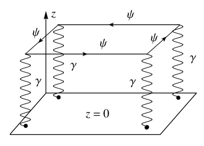
Figure 1: Light by light scattering amplitude in a domain wall set up, $\mathcal{M}(\gamma\gamma\!\rightarrow\!\gamma\gamma)\!\propto\!L\rightarrow\infty$.

The organization of this paper is as follows. In Sec. II we consider 5D spinor QED with gauge field localized on the domain wall. We introduce the model in Sec. II.1 and in Sec. II.2 we explicitly calculate one loop fermion correction to the vector brane-to-brane propagator. In Sec. III we consider 6D spinor QED in the background of RSII-1 metric with one compact extra dimension $\theta$ and one infinite extra dimension $z$. We calculate the vector propagator in Sec. III.1. In Sec. III.2 we derive one loop contribution of $\theta$-homogeneous KK fermions into the vector brane-to-brane propagator. In Sec. III.3 we discuss a position depenent cutoff scheme for calculating the one loop contribution of $\theta$-inhomogeneous KK excitations of fermions to the vector propagator, and calculate this correction explicitly. We conclude in Sec. IV. Technical details are collected in Appendices.

II Domain wall set up

II.1 The model

In this section we consider Euclidean 5D brane-world model with fermion and vector fields propagating in the bulk Smolyakov:2011hv . The action of the model is

$$S\!=\!\!\int\!\!d^{4}x\,dz\Bigl{[}\,\frac{1}{4}\phi^{2}(z)F_{MN}^{2}+i\overline{\Psi}\Gamma^{M}(\partial_{M}-i{\mathrm{g}}_{5}A_{M})\Psi\Bigr{]},$$ (1)

where indices $M,N$ label 5D space, $M,N=0,1,2,3,5$, and

$$\phi(z)=1/{\rm ch}\alpha z$$ (2)

is a field configuration which ensures the localization of vector zero mode on the brane; the parameter $1/\alpha$ is related to the brane thickness. This mechanism of gauge field localization on a higher dimensional deffect is analogous to those considered in Ref. Barnaveli:1990bi . For simplicity we assume that the fermions propagate in the flat 5D bulk. 5D and 4D couplings are related by

$${\mathrm{g}}_{5}=\frac{1}{\sqrt{\alpha}}{\mathrm{g}}_{4}.$$ (3)

It is convenient to introduce the new field $B_{M}$, which is related to $A_{M}$ as follows:

$$B_{M}=\phi A_{M}.$$ (4)

The Lagrangian of the vector field $B_{M}$ can be written as follows:

$$\begin{split}\mathcal{L}\!=\!\frac{1}{2}B_{\mu}\!\left[\eta_{\mu\nu}\!\left(\!-\partial^{2}_{\lambda}\!-\!\partial^{2}_{z}\!+\!\frac{\phi^{\prime\prime}}{\phi}\right)\!\!+\!\partial_{\mu}\partial_{\nu}\right]\!\!B_{\nu}-\\ -\frac{1}{2}B_{z}\partial^{2}_{\mu}B_{z}-B_{z}\!\left(\frac{\phi^{\prime}}{\phi}-\partial_{z}\right)\!\!\partial_{\mu}B_{\mu},\end{split}$$ (5)

where Greek indices refer to 4D, $\mu,\nu=0,1,2,3$. We set the gauge $B_{z}=0$, then the vector field $B_{\mu}$ is transverse, $\partial_{\mu}B_{\mu}=0$. KK modes $B^{(m)}(z)$ of the vector field $B_{\mu}$ obey

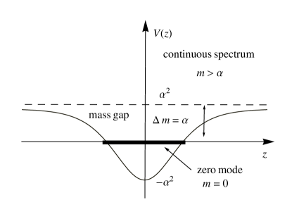
Figure 2: Domain wall effective potential.

$$\left(-\partial^{2}_{z}+\frac{\phi^{\prime\prime}}{\phi}\right)B^{(m)}(z)=m^{2}B^{(m)}(z).$$ (6)

where $m$ is 4D mass. The mass spectrum is determined by the quantum-mechanical potential

$$V(z)=\frac{\phi^{\prime\prime}}{\phi}=\alpha^{2}-\frac{2\alpha^{2}}{{\rm ch}^{2}\alpha z}.$$

In this potential the vector field has one bound state (see Fig. 2), which is actually the zero mode,

$$B^{(0)}(z)=\sqrt{\frac{\alpha}{2}}\frac{1}{{\rm ch}\,\alpha z}.$$ (7)

This mode is normalized with unit measure, in accordance with the Lagrangian (5). Eq. (6) has also solutions $B^{(m)}(z)$, which correspond to the continuous spectrum starting from $m=\alpha$. Therefore, the zero mode $B^{(0)}(z)$ is separated from higher modes $B^{(m)}(z)$ by non-zero mass gap $\Delta m=\alpha$.

Now let us consider the propagator of the vector field $B_{\mu}$ from brane to bulk, $G^{B}_{\mu\nu}(p,z,0)=\langle B_{\mu}(p,z)B_{\nu}(p,0)\rangle$. This propagator obeys

$$\left(p^{2}-\partial^{2}_{z}+\alpha^{2}-\frac{2\alpha^{2}}{{\rm ch}^{2}\alpha z}\right)G^{B}_{\mu\nu}(p,z,0)=\eta_{\mu\nu}\delta(z).$$ (8)

The solution to Eq. (8) is $G^{B}_{\mu\nu}(p,z,0)=\eta_{\mu\nu}G_{B}(p,z,0)$, where (see Appendix A)

$$G_{B}(p,z,0)=\frac{1}{4\,{\rm ch}\alpha z}\left(\frac{{\rm e}^{-(\chi-\alpha)|z|}}{\chi-\alpha}+\frac{{\rm e}^{-(\chi+\alpha)|z|}}{\chi+\alpha}\right),$$ (9)

and

$$\chi=\sqrt{p^{2}+\alpha^{2}}.$$ (10)

It is worth noting that brane-to-bulk propagator of the vector field $A_{\mu}(p,z)$ is

$$\begin{split}\langle A_{\mu}(p,z)A_{\nu}(p,0)\rangle&=\eta_{\mu\nu}G_{B}(p,z,0)/\phi(z)\\ &\equiv\eta_{\mu\nu}G_{A}(p,z,0),\end{split}$$ (11)

where

$$G_{A}(p,z,0)=\frac{1}{4}\left(\frac{{\rm e}^{-(\chi-\alpha)|z|}}{\chi-\alpha}+\frac{{\rm e}^{-(\chi+\alpha)|z|}}{\chi+\alpha}\right).$$ (12)

Vector fields $A_{M}$ and $B_{M}$ coincide on the brane $z=0$, their propagators from brane to brane coincide as well

$$G_{A}(p,0,0)=G_{B}(p,0,0)=\chi/(2p^{2}).$$ (13)

At low energy, $p\ll\alpha$, only zero mode of gauge field is relevant, and the propagator (13) takes the form

$$G_{A}(p,0,0)=\alpha/(2p^{2}).$$ (14)

It follows from Eqs. (10) and (12) that at small $p$

$$G_{A}(p,z,0)=\frac{\alpha}{2p^{2}}\exp{\left(-\frac{p^{2}|z|}{2\alpha}\right)},$$ (15)

hence the bulk vector Green’s function $G_{A}(p,z,0)$ decreases slowly towards $z\rightarrow\infty$ in the IR regime. We will also use the propagator $G_{A}(p,z,0)$ in the momentum space

$$\begin{split}&\widetilde{G}_{A}(p,p_{z})=\int\limits_{-\infty}^{+\infty}\!dz\,G_{A}(p,z,0)\,{\rm e}^{ip_{z}z}\\ &=\frac{1}{2}\left(\frac{1}{(\chi\!-\!\alpha)^{2}\!+\!p_{z}^{2}}+\frac{1}{(\chi\!+\!\alpha)^{2}\!+\!p_{z}^{2}}\right).\end{split}$$ (16)

We find from Eqs. (10) and (16), that as $p_{z}\rightarrow\leavevmode\nobreak\ 0$ and $p/\alpha\ll 1$, then the brane-to-bulk vector propagator in the momentum space tends to

$$\widetilde{G}_{A}(p,p_{z})=\frac{1}{2}\frac{1}{(p_{z}^{2}+p^{4}/(4\alpha^{2}))}.$$ (17)

We note that Eq. (17) differs considerably from the vector propagator in the flat 5D space

$$\widetilde{G}^{flat}_{A}(p,p_{z})=\frac{1}{p^{2}+p_{z}^{2}}.$$ (18)

In Sec. II.2 we show that the term $p^{4}/(4\alpha^{2})$ in Eq. (17) leads to IR pathology of the one-loop vector brane-to-brane propagator.

II.2 One loop fermion contribution to the vector brane-to-brane propagator

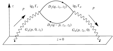
Figure 3: One loop correction to the vector brane-to-brane propagator.

In this section we calculate the one loop fermion contribution to the vector propagator from brane to brane (see Fig. 3). The coupling of the fields $A_{\mu}$ and $\Psi$ is

$$S_{int}[\Psi,A]=\int d^{4}x\,dz\,{\mathrm{g}}_{5}\overline{\Psi}\,\Gamma^{\mu}A_{\mu}\Psi.$$ (19)

One loop brane-to-brane vector Green’s function is

$$\mathcal{G}_{\mu\nu}(p)=G^{(0)}_{\mu\nu}(p)+G_{\mu\nu}^{(1)}(p),$$ (20)

where tree level propagator is $G^{(0)}_{\mu\nu}(p)\equiv\eta_{\mu\nu}G_{A}(p,0,0)$, and one loop contribution $G_{\mu\nu}^{(1)}(p)$ is given by

$$\begin{split}&G_{\mu\nu}^{(1)}(p)\!=\!(i{\mathrm{g}}_{5})^{2}\!\!\!\int\limits_{-\infty}^{\infty}\!\!dz_{1}\!\!\!\int\limits_{-\infty}^{\infty}\!\!\!dz_{2}\,G_{A}(p,z_{1},0)G_{A}(p,z_{2},0)\times\\ &\times\!\!\int\!\!\frac{d^{4}q}{(2\pi)^{4}}\!(-1)\mathrm{Tr}\left[\Gamma_{\mu}D_{f}(q-p,z_{1},z_{2})\Gamma_{\nu}D_{f}(q,z_{1},z_{2})\right].\end{split}$$ (21)

Green’s function of massless 5D fermions $D_{f}(q,z_{1},z_{2})$ has the form

$$D_{f}(q,z,z^{\prime})=\int\limits_{-\infty}^{\infty}\frac{dq_{z}}{2\pi}\frac{\widehat{Q}}{Q^{2}}\,{\rm e}^{iq_{z}(z-z^{\prime})},$$ (22)

where $\widehat{Q}=\Gamma^{M}q_{M}=\Gamma^{\mu}q_{\mu}+\Gamma^{z}q_{z}$, $Q^{2}$ is 5D momentum squared, $Q^{2}=q^{2}+q_{z}^{2}$. Therefore, the one loop fermion contribution (21) can be written as follows

$$G^{(1)}_{\mu\nu}(p)\!=\!({\mathrm{g}}_{5})^{2}\!\!\!\int\limits_{-\infty}^{\infty}\frac{dp_{z}}{2\pi}\left|\widetilde{G}_{A}(p,p_{z})\right|^{2}\widetilde{\Pi}_{\mu\nu}(p,p_{z}).$$ (23)

where $\widetilde{G}_{A}(p,p_{z})$ is given by Eq. (16) and $\widetilde{\Pi}_{\mu\nu}$ is vacuum polarization operator in flat 5D space with 4D indices:

$$\widetilde{\Pi}_{\mu\nu}(p,p_{z})=\int\!\!\frac{d^{5}Q}{(2\pi)^{5}}\frac{{\tt Tr}\Bigl{[}\Gamma_{\mu}\widehat{Q}\Gamma_{\nu}(\widehat{Q}-\widehat{P})\Bigr{]}}{Q^{2}(Q-P)^{2}}.$$ (24)

We make use of dimensional regularization and obtain

$$\widetilde{\Pi}_{\mu\nu}(p,p_{z})=\frac{3\pi}{64}\,\frac{2^{2}}{(4\pi)^{2}}P\Bigl{(}\eta_{\mu\nu}P^{2}-p_{\mu}p_{\nu}\Bigr{)}.$$ (25)

where 5D momentum squared is

$$P^{2}=p^{2}+p_{z}^{2}.$$ (26)

Let us consider the one loop correction $G^{(1)}_{\mu\nu}(p)$ in the low energy limit, $p\rightarrow 0$. We substitute Eqs. (16) and (25) into Eq. (23) and integrate (23) over $p_{z}$, then we get

$$\begin{split}G^{(1)}_{\mu\nu}(p)\!=&\frac{(g_{4})^{2}}{2\pi}\frac{3\pi}{64}\frac{2^{2}}{(4\pi)^{2}}\frac{\alpha}{2p^{2}}\Big{[}\left(\!\eta_{\mu\nu}\!-\!\frac{p_{\mu}p_{\nu}}{p^{2}}\right)\!Q_{T}(p)+\\ &+\frac{p_{\mu}p_{\nu}}{p^{2}}Q_{L}(p)\Big{]}.\end{split}$$ (27)

The factor $\alpha/(2p^{2})$ in Eq. (27) is due to the vector zero mode (see Eq. (14)). Functions $Q_{T}(p)$ and $Q_{L}(p)$ are defined by

$$\begin{split}Q_{T}(p)\!=\!\!\int\limits_{-\infty}^{+\infty}\!\!dp_{z}\frac{2p^{2}}{\alpha^{2}}P^{3}\Bigl{|}\widetilde{G}_{A}(p,p_{z})\Bigr{|}^{2},\\ Q_{L}(p)\!=\!\!\int\limits_{-\infty}^{+\infty}\!\!dp_{z}\frac{2p^{2}}{\alpha^{2}}Pp_{z}^{2}\Bigl{|}\widetilde{G}_{A}(p,p_{z})\Bigr{|}^{2}.\end{split}$$ (28)

One obtains in IR regime $p\rightarrow 0$

$$\begin{split}&Q_{T}(p)=\frac{2\pi\alpha}{p}+\frac{9\pi p}{4\alpha}+\\ &+\frac{p^{2}}{\alpha^{2}}\left(4\,{\mathrm{ln}}\frac{2\Lambda}{p}+3{\mathrm{ln}}\frac{p}{4\alpha}-\frac{11}{6}\right)+O\left(\frac{p^{3}}{\alpha^{3}}\right)\end{split}$$ (29)

$$Q_{L}(p)\!=\!\frac{\pi p}{2\alpha}\!+\!\frac{p^{2}}{\alpha^{2}}\!\left(\!4{\mathrm{ln}}\frac{2\Lambda}{p}\!+\!3{\mathrm{ln}}\frac{p}{4\alpha}\!-\!\frac{3}{2}\right)\!+\!O\!\left(\!\frac{p^{3}}{\alpha^{3}}\!\right),$$ (30)

where $\Lambda$ is the UV cutoff scale. It follows from Eq. (29) that in the low energy limit $p/\alpha\ll 1$ the function $Q_{T}(p)$ is proportional to $\alpha/p$. The reason for this singularity is as follows. We have pointed out in Sec. II.1 that brane-to-bulk propagator $\widetilde{G}_{A}(p,p_{z})$ has a peculiar term $p^{4}/(4\alpha^{2})$ in the denominator as $p_{z}\rightarrow 0$ (see Eq. (17)). This means that the integral (28) for $Q_{T}(q)$ has the following IR contribution:

$$Q_{T}(p)\propto\int\limits_{-\infty}^{+\infty}\!\!dp_{z}\frac{p^{2}}{\alpha^{2}}\frac{(p_{z}^{2}+p^{2})^{3/2}}{(p_{z}^{2}\!+\!p^{4}/(4\alpha^{2}))^{2}}.$$ (31)

This integral is saturated in IR region at $p_{z}\sim p^{2}/\alpha$, hence

$$Q_{T}(p)\propto\frac{p^{2}}{\alpha^{2}}\frac{(p^{2}/\alpha)p^{3}}{(p^{8}/\alpha^{4})}\propto\frac{\alpha}{p},$$ (32)

which coincides with Eq. (29). Therefore, the one loop contribution of massless fermions to the vector brane-to-brane propagator is

$$G_{\mu\nu}^{(1)}(p)=\frac{3({\mathrm{g}}_{4})^{2}}{2^{9}\pi}\frac{\alpha^{2}}{p^{3}}\left(\eta_{\mu\nu}-\frac{p_{\mu}p_{\nu}}{p^{2}}\right),$$ (33)

while the tree level propagator $G_{A}(p,0,0)$ is propotional to $1/p^{2}$ (see Eq. (13)). This means that the model is inconsistent in the IR limit. One way to interpret the result (33) is to claim that the theory is in the strong coupling regime at $({\mathrm{g}}_{4})^{2}\alpha/p\lesssim 1$, where the one loop correction exceeds the tree level propagator. We conclude that the model with mass gap between zero and massive vector KK modes is pathological in IR, as expected.

III RSII-1 set up

In this section we consider a model without mass gap between zero and massive vector KK modes. Namely, we calculate the one loop contribution of massles fermions to the brane-to-brane vector propagator in the framework of RSII-1 model with one compact and one infinite extra dimensions. 6D mectric of Euclidean RSII-1 model is

$$\begin{split}ds^{2}&=G_{MN}dx^{M}dx^{N}\\ &=w^{2}(z)(\eta_{\mu\nu}dx^{\mu}dx^{\nu}+d\theta^{2}+dz^{2}),\end{split}$$ (34)

where indices $M,N$ denote the coordinates of 6D spacetime, $M,N=0,1,2,3,5,6$. Greek indices $\mu,\nu$ label 4D subspace, $\mu,\nu=0,1,2,3$, $x^{5}$ is the compact extra dimension, $x^{5}\equiv\theta\in[0,2\pi R]$, and $x^{6}\equiv z$ refers to extra dimension of infinite size $z\in[-\infty,+\infty]$. The warp factor $w(z)$ is given by

$$w(z)=1/(1+k|z|).$$ (35)

From geometric point of view, the metric (34) describes 5-brane with one compact dimension located at the point $z=0$ of bulk space. Let us consider the action of $U(1)$ gauge theory with massles fermions in the background (34)

$$\begin{split}S_{RS}[\psi,A]=\int d^{4}x\,dz\,d\theta\sqrt{G}\Big{[}\frac{1}{4}F_{MN}F^{MN}+\\ +\,i\overline{\psi}\Gamma^{\bar{M}}E_{\bar{M}}^{M}(\nabla_{M}-i{\mathrm{g}}_{6}A_{M})\psi\Big{]},\end{split}$$ (36)

where indices $\bar{M},\bar{N}$ label the tangent space and $\nabla_{M}$ is spinorial covariant derivative. Couplings and fields have the following mass dimensions: $[{\mathrm{g}}_{6}]=-1$, $[A_{M}]=2$ and $[\Psi]=5/2$. The size of compact extra dimension $R$ is assumed to be $R\ll 1/E$, where $E$ is the energy of interest. In Secs. III.1 and III.2 we study KK excitations of fermions and bosons which are homogeneous along the compact extra dimension $\theta$. We discuss in Sec. III.3 quantum corrections to the photon propagator coming from the fermion states inhomogeneous along $\theta$.

III.1 Vector field propagator in the RSII-1 set up

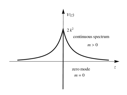
Figure 4: RSII-1 effective potential.

Let us find brane-to-bulk vector Green’s function. The vector part of the action (36) is

$$S[A]=\int d^{4}x\,dz\,d\theta\,w^{2}(z)\,\frac{1}{4}F_{MN}^{2},$$ (37)

where indices $M,N$ are contracted with flat metric. The action (37) is analogous to that considered in domain wall set up (see vector part of the action (1)) expect for the form of the warp factor $w(z)$. We introduce the vector field $B_{M}$ in the same way as in Sec. II.1 (see Eq. (4))

$$B_{M}=wA_{M}.$$ (38)

We consider the field $B_{M}$ independent of $\theta$ with $B_{\theta}=0$ and choose the gauge $B_{z}=0$.

The equation of motion for KK mode $B^{(m)}(z)$ of the field $B_{\mu}(x,z)$ coincides with Eq. (6) up to redefinition $\phi(z)\rightarrow w(z)$. In RSII-1 set up the spectrum is determined by quantum - mechanical potential (see Fig. 4)

$$V(z)=\frac{w^{\prime\prime}}{w}=\frac{2k^{2}}{(1\!+\!k|z|)^{2}}-2k\,\delta(z).$$ (39)

Vector field $B^{(m)}(z)$ has a zero mode

$$B^{(0)}(z)=\sqrt{\frac{k}{2}}\frac{1}{(1\!+\!k|z|)},$$ (40)

which has to do the delta function well in $V(z)$. This zero mode corresponds to the constant field $A^{(0)}(z)=\sqrt{k/2}$. The latter is homogeneous along the large extra dimension $z$ and represents the photon localized on the brane. In contrast to the domain wall set up, there is no mass gap, separating the zero mode $B^{(0)}(z)$ from the continuum of states $B^{(m)}(z)$.

The brane-to-bulk vector Green’s function $G^{B}_{\mu\nu}(p,z,0)=\langle B_{\mu}(p,z)B_{\nu}(p,0)\rangle$ obeys

$$\left(p^{2}\!-\!\partial_{z}^{2}\!+V(z)\right)G^{B}_{\mu\nu}(p,z,0)=\eta_{\mu\nu}\delta(z),$$ (41)

We obtain the solution to Eq. (41) in Appendix B. It is given by $G^{B}_{\mu\nu}(p,z,0)=\eta_{\mu\nu}G_{B}(p,z,0)$, where

$$G_{B}(p,z,0)=\frac{{\rm e}^{-p|z|}}{2p}+\!\frac{k{\rm e}^{-p|z|}}{2p^{2}}\frac{1}{(1\!+\!k|z|)}.$$ (42)

The first term in Eq. (42) is the Green’s function of massles field in flat 5D spacetime. The second term of Eq. (42) is proportional to $1/p^{2}$, therefore this is the zero mode contribution to the vector propagator at the tree level. In the IR regime $p/k\ll 1$, brane-to-bulk propagator of the field $A_{\mu}$ has the form

$$G_{A}(p,z,0)\equiv G_{B}(p,z,0)/w(z)=\frac{k}{2p^{2}}\exp(-p|z|).$$ (43)

In contrast to the domain wall case (see Eq. (15)) $G_{A}(p,z,0)$ of RSII-1 set up decreases more rapidly towards $z\rightarrow\infty$ in IR limit. It is worth rewriting the Green’s function $G_{A}(p,z,0)$ in the momentum space:

$$\widetilde{G}_{A}(p,p_{z})\!=\!\!\int\limits_{-\infty}^{\infty}\!dz\,G_{A}(p,z,0)e^{ip_{z}z}\!=\frac{1}{P^{2}}+\frac{2pk}{P^{4}},$$ (44)

where $P$ is defined by Eq. (26).

III.2 One loop contribution of $\theta$-homogeneous fermions to the vector brane-to-brane propagator.

In this section we derive one loop fermion correction to the vector Green’s function from brane-to-brane. It is known that massless fermions are conformal, i. e., upon rescaling of the fermion field

$$\psi=w^{-5/2}\Psi,$$ (45)

the fermion action reduces to the flat-space form

$$S[\Psi]\!=\!\!\int\!\!d^{4}x\,dz\,d\theta\!\left(i\overline{\Psi}\Gamma^{\mu}\partial_{\mu}\Psi\!+\!i\overline{\Psi}\Gamma^{\theta}\partial_{\theta}\Psi\!+\!i\overline{\Psi}\Gamma^{z}\partial_{z}\Psi\right).$$ (46)

where $\Gamma^{\mu}$, $\Gamma^{\theta}$ and $\Gamma^{z}$ are Euclidean 6D gamma matrices; $\Psi$ is eight-component Dirac spinor

$$\Psi=\left(\Psi_{+},\Psi_{-}\right),$$

where $\Psi_{+}$ and $\Psi_{-}$ are four-component spinors which have appropriate signs of 6D chirality. Consider now the KK mode expansion

$$\Psi(x,z,\theta)=\frac{1}{\sqrt{2\pi R}}\Psi^{0}(x,z)+\sum_{n\neq 0}\Psi^{n}(x,z)f_{S}^{n}(\theta).$$ (47)

where $\Psi^{0}(x,z)$ and $\Psi^{n}(x,z)f_{S}^{n}(\theta)$ are $\theta$-homogeneous and $\theta$-inhomogeneous KK modes, respectively. We have dropped 6D chirality indices $(\pm)$ in Eq. (47) for simplicity. Integrating out the compact extra dimension, one obtains

$$\begin{split}S[\Psi]\!=\!\int\!\!d^{4}xdzd\theta\sum_{n}\Big{(}i\overline{\Psi}^{n}\Gamma^{\mu}\partial_{\mu}\Psi^{n}+\\ +\ i\overline{\Psi}^{n}\Gamma^{z}\partial_{z}\Psi^{n}+im_{n}\overline{\Psi}^{n}\Psi^{n}\Big{)},\end{split}$$ (48)

where $m_{n}=n/R$ is the mass of KK state.

Let us consider the one loop correction to the vector propagator coming from the $\theta$-homogeneous state $\Psi^{0}$. The interaction of $\Psi^{0}(x,z)$ and $A_{\mu}(x,z)$ is described by the action

$$S[A,\Psi^{0}]\!=\!\!\int\!\!d^{4}x\,dz\,{\mathrm{g}}_{5}\,\overline{\Psi}^{0}\!(x,z)\Gamma^{\mu}A_{\mu}(x,z)\Psi^{0}(x,z),$$ (49)

where ${\mathrm{g}}_{5}$ is the 5D coupling

$${\mathrm{g}}_{5}=\frac{{\mathrm{g}}_{6}}{\sqrt{2\pi\!R}}$$ (50)

with mass dimension $[{\mathrm{g}}_{5}]=-1/2$.

The action (49) is analogous to the vector-fermion coupling in the domain wall set up (see Eq. 19). Since there are two types of four-component Dirac spinors in 6D model, one can carry over Eqs. (19) - (28) to the RSII-1 scenario up to the fermion doubling factor in Eq. (25)

$$\widetilde{\Pi}_{\mu\nu}(p,p_{z})\rightarrow 2\widetilde{\Pi}_{\mu\nu}(p,p_{z}).$$

Upon substituting Eqs. (44) and (25) into Eq. (23), one gets

$$\begin{split}G_{\mu\nu}^{(1)}(p)&=\!\frac{({\mathrm{g}}_{4})^{2}}{2\pi}\frac{3\pi}{64}\,\frac{2^{3}}{(4\pi)^{2}}\frac{k}{2p^{2}}\Big{[}\left(\!\eta_{\mu\nu}\!-\!\frac{p_{\mu}p_{\nu}}{p^{2}}\!\right)\!Q_{T}(p)+\\ &+\frac{p_{\mu}p_{\nu}}{p^{2}}\,Q_{L}(p)\Big{]},\end{split}$$ (51)

where 5D and 4D effective couplings are related by Eq. (3) up to the redefinition $\alpha\rightarrow k$. The functions $Q_{T}(p)$ and $Q_{L}(p)$ are defined by Eq. (28) with $\widetilde{G}(p,p_{z})$ given by Eq. (44) . Then, after integrating Eq. (28) over $p_{z}$, one finds

$$\begin{split}&Q_{T}(p)=\!\frac{32}{3}+\frac{16\,p}{k}+\frac{4p^{2}}{k^{2}}{\mathrm{ln}}\frac{2\Lambda}{p},\\ &Q_{L}(p)\!=\!\frac{32}{15}+\frac{16}{3}\frac{p}{k}+\frac{4p^{2}}{k^{2}}\left(\!{\mathrm{ln}}\frac{2\Lambda}{p}-1\right),\end{split}$$ (52)

Therefore, the one loop fermion contribution $G^{(1)}_{\mu\nu}(p)$ to the vector brane-to-brane propagator $G^{(0)}_{\mu\nu}(p)$ (cf. Eq. (42) at $z=0$) in IR regime is given by

$$G^{(1)}_{\mu\nu}(p)=\frac{({\mathrm{g}}_{4})^{2}}{(4\pi)^{2}}\frac{k}{p^{2}}\left(\eta_{\mu\nu}-\frac{4}{5}\frac{p_{\mu}p_{\nu}}{p^{2}}\right).$$ (53)

It is worth noting that both $G^{(1)}_{\mu\nu}(p)$ and $G^{(0)}_{\mu\nu}(p)$ are proportional to $k/p^{2}$ as $p\rightarrow 0$. This means that there is no IR singularity in the one loop vector brane-to-brane propagator of the RSII-1 set up. This is in contrast to Sec. II.

One can understand the IR behaviour of $G^{(1)}_{\mu\nu}(p)$ in a way analogous to that considered in Sec. II.2. Namely, let us consider Eq. (28) in the case of RSII-1 model. From (44) it follows that if $P\rightarrow 0$ then $\widetilde{G}_{A}(p,p_{z})\propto kp/P^{4}$. Hence the main IR contributions to $Q_{T}(p)$ and $Q_{L}(p)$ come from the integrals

$$\begin{split}Q_{T}(p)\propto\!\!\!\int\limits_{-\infty}^{+\infty}\!\!dp_{z}\frac{p^{2}}{k^{2}}\!\!\left[\frac{kp}{(p_{z}^{2}+p^{2})^{2}}\right]^{2}\!\!(p_{z}^{2}+p^{2})^{3/2},\,\,\\ Q_{L}(p)\propto\!\!\!\int\limits_{-\infty}^{+\infty}\!\!dp_{z}\frac{p^{2}}{k^{2}}\!\!\left[\frac{kp}{(p_{z}^{2}+p^{2})^{2}}\right]^{2}\!\!(p_{z}^{2}+p^{2})^{1/2}p_{z}^{2},\end{split}$$ (54)

These integrals are saturated at $p_{z}\sim p$, therefore one has

$$Q_{T}(p)\propto Q_{L}(q)\propto p\,\frac{p^{2}}{k^{2}}\frac{k^{2}p^{2}}{p^{8}}p^{3}\propto O(1)$$ (55)

which coincides with Eq. (52) for $p/k\ll 1$.

Thus, the analysis of the one loop vector propagators in the two brane world models shows that the IR behaviour of vector brane-to-brane propagators is in one-to-one correspondence with the existence of the mass gap. While there is IR pathology in the model with the gap, the gapless model is IR healthy.

III.3 Contribution of $\theta$-inhomogeneous KK fermions.

In this section we derive one loop contribution of $\theta$-inhomogeneous fermions to the vector brane-to-brane propagator. Since the masses of corresponding KK excitations are large, $m_{n}=n/R\gg p$, production of heavy inhomogeneous fermion modes is forbidden at the tree-level. Nevertheless, these modes may contribute to the vector brane-to-brane propagator at the one loop level.

Let us recall that RSII-1 model is a 6D non-renormalizable spinor QED with warped extra dimension. If the set up were 6D spinor QED on flat background, we would have to impose the following condition on gauge coupling ${\mathrm{g}}_{6}$ and UV cutoff scale $\Lambda$

$$\Lambda\ll 1/{\mathrm{g}}_{6}.$$ (56)

In warped space-time, it is appropriate to use the position dependent cutoff formalizm Randall:2001gb . Namely, the cutoff scale at given $z$ is $\Lambda_{\tt eff}(z)=\Lambda/(1\!+\!kz)$. In particular, one imposes position dependent upper bound on KK masses

$$m_{n}<\Lambda/(1\!+\!kz).$$ (57)

Thus, the one-loop contribution of $\theta$-inhomogeneous KK states can be written as follows:

$$\begin{split}G_{\mu\nu}^{KK}(p)&=\!({\mathrm{g}}_{5})^{2}\!\!\!\int\limits_{-\infty}^{+\infty}\!\!dz_{1}dz_{2}\,G_{A}(p,\!z_{1},\!0)G_{A}(p,\!z_{2},\!0)\times\\ &\times\int\limits_{-\infty}^{+\infty}\!\frac{dp_{z}}{2\pi}\,{\rm e}^{ip_{z}(z_{1}-z_{2})}\!\!\!\!\sum_{n\neq 0}^{N_{KK}(z)}\!\!\!\widetilde{\Pi}_{\mu\nu}^{n}(p,p_{z}),\end{split}$$ (58)

where $N_{KK}(z)$ is the effective number of KK states, and $z=(z_{1}\!+\!z_{2})/2$; $\widetilde{\Pi}_{\mu\nu}^{n}(p,p_{z})$ is the one loop fermion integral of massive KK excitations (compare with massless case Eq. (24) and (25))

$$\widetilde{\Pi}^{n}_{\mu\nu}(p,p_{z})\!=\!\!\!\int\limits_{0}^{1}\!\!dx\frac{2^{3}}{(4\pi)^{2}}\,2\sqrt{\Delta_{n}}\!\left(\eta_{\mu\nu}P^{2}\!-\!p_{\mu}p_{\nu}\!\right)x(1-x),$$ (59)

where $\Delta_{n}=m_{n}^{2}+x(1-x)P^{2}$. Since $m_{n}\gg p$, we set $\Delta_{n}=m_{n}^{2}$ in Eq. (59), and then evaluate the integral. In this way we obtain in IR regime $P\ll k$

$$\widetilde{\Pi}^{n}_{\mu\nu}(p,p_{z})=\frac{2^{3}}{(4\pi)^{2}}\,2\,\frac{m_{n}}{6}\left(\eta_{\mu\nu}P^{2}-p_{\mu}p_{\nu}\right),$$ (60)

Let us use the variables $z=(z_{1}\!+\!z_{2})/2$ and $z^{\prime}=z_{1}\!-\!z_{2}$ in Eq. (58). Implementing the cutoff condition (57), we interchange the order of bulk space integration and KK summation in Eq. (58). Then, after integrating over $p_{z}$, we have

$$\begin{split}&G^{KK}_{\mu\nu}(p)\!=\!({\mathrm{g}}_{5})^{2}\!\!\sum_{n\neq 0}^{N_{KK}}\!\!\frac{m_{n}}{6}\!\!\!\int\limits_{-z_{IR}^{n}}^{+z_{IR}^{n}}\!\!\!\!dz\,dz^{\prime}\delta(z^{\prime})\frac{2^{3}}{(4\pi)^{2}}2\,\times\\ &\times\left[\left(\eta_{\mu\nu}p^{2}\!-\!p_{\mu}p_{\nu}\right)\!-\!\eta_{\mu\nu}\frac{\partial^{2}}{\partial z^{\prime 2}}\right]\times\\ &\times G_{A}(p,z\!+\!z^{\prime}/2,0)G_{A}(p,z\!-\!z^{\prime}/2,0),\end{split}$$ (61)

where $z_{IR}^{n}=(\Lambda-m_{n})/(km_{n})$, the masses of KK states are bounded now by $m_{n}<\Lambda$. Hence, the number of KK states in (61) is

$$N_{KK}=R\Lambda.$$ (62)

Integrating Eq. (61) over $z^{\prime}$ and $z$, one obtains

$$\begin{split}G^{KK}_{\mu\nu}(p)\!=&\!({\mathrm{g}}_{5})^{2}\!\!\sum_{n\neq 0}^{N_{KK}}\!\!\frac{m_{n}}{6}\frac{2^{3}}{(4\pi)^{2}}\!\Big{(}\left[\eta_{\mu\nu}\!-\!\frac{p_{\mu}p_{\nu}}{p^{2}}\right]\!\mathcal{F}^{n}_{1}(p)+\\ &+\eta_{\mu\nu}\mathcal{F}^{n}_{2}(p)\Big{)},\end{split}$$ (63)

where $\mathcal{F}^{n}_{1}(p)$ and $\mathcal{F}^{n}_{2}(p)$ are given by

$$\begin{split}\mathcal{F}^{n}_{1}(p)&=\frac{5}{8}\frac{k^{2}}{p^{3}}(1-{\rm e}^{-pz_{IR}^{n}})+\frac{3}{8}\frac{k}{p^{2}}\Big{(}2(1-{\rm e}^{-pz_{IR}^{n}})-\\ &-{\rm e}^{-pz_{IR}^{n}}kz_{IR}^{n}\Big{)}+\frac{1}{16p}\Big{(}4(1-{\rm e}^{-pz_{IR}^{n}})-\\ &-4{\rm e}^{-pz^{n}_{IR}}kz^{n}_{IR}-{\rm e}^{-pz_{IR}^{n}}(kz_{IR}^{n})^{2}\Big{)}\end{split}$$ (64)

$$\begin{split}\mathcal{F}^{n}_{2}(p)&=\frac{k}{2p^{2}}{\rm e}^{-pz_{IR}^{n}}\bigl{(}1+kz_{IR}^{n}/2\bigr{)}+\\ &+\frac{1}{2p}{\rm e}^{-pz_{IR}^{n}}\bigl{(}1+kz_{IR}^{n}+(kz_{IR}^{n})^{2}/4\bigr{)}.\end{split}$$ (65)

Let us consider low momentum regime $pz_{IR}^{n}\ll 1$, then at $p/k\ll 1$ one has

$$\mathcal{F}_{1}^{n}(p)=\mathcal{F}_{2}^{n}(p)=\frac{z_{IR}^{n}}{4}\frac{k^{2}}{p^{2}}.$$

Therefore

$$G^{KK}_{\mu\nu}(p)=\frac{({\mathrm{g}}_{4})^{2}}{48\pi^{2}}\sum_{n\neq 0}^{N_{KK}}\frac{(\Lambda-m_{n})}{p^{2}}\left(2\eta_{\mu\nu}-\frac{p_{\mu}p_{\nu}}{p^{2}}\right),$$

which leads to

$$G^{KK}_{\mu\nu}(p)=\frac{({\mathrm{g}}_{4})^{2}}{48\pi^{2}}\frac{\Lambda(\Lambda R+1)}{2p^{2}}\left(2\eta_{\mu\nu}-\frac{p_{\mu}p_{\nu}}{p^{2}}\right)$$ (66)

It follows from Eq. (50) and Eq. (3) that 6D and 4D couplings are related by

$${\mathrm{g}}_{6}={\mathrm{g}}_{4}\sqrt{\frac{2\pi R}{k}},$$

therefore Eq. (66) is finally written as

$$G^{KK}_{\mu\nu}(p)=\frac{({\mathrm{g}}_{6}\Lambda)^{2}}{192\pi^{3}}\frac{k}{p^{2}}\left(2\eta_{\mu\nu}-\frac{p_{\mu}p_{\nu}}{p^{2}}\right).$$ (67)

This is indeed a small correction to the tree-level propagator, provided that $({\mathrm{g}}_{6}\Lambda)^{2}\ll 1$, which coincides with Eq. (56). We conclude that the entire RSII-1 scenario is viable at least at the one loop level.

IV Discussion and conclusion

In this paper we have considered two brane-world models with different mechanisms of gauge field localization on the brane. We found that the fermion one loop correction to the vector brane-to-brane propagator has a pathological IR divergence in the framework of 5D massles spinor QED with gauge field localized on the domain wall, which makes this model inconsistent. This result is consistent with the observation in Ref. Smolyakov:2011hv . We have also considered 6D massles spinor QED in the background of modified Randall-Sundrum metric. We have explicitly calculated the one loop fermion cotribution to the vector brane-to-brane propagator in this framework in the low energy limit. This contribution is healthy in IR, so one can consider the RSII-1 set up as consistent brane world scenario, at least at the one loop level.

We conclude that IR are inherent in models with gauge field zero mode separated from heavier modes by a gap, while models without the gap may be healthy in IR.

V Acknowledgements

We are indebted to D. S. Gorbunov, A. L. Kataev, M. Y. Kuznetsov, D. G. Levkov, A. G. Panin, V. A. Rubakov and M. A. Smolyakov for helpful discussions. This work was supported in part by grants of Russian Ministry of Education and Science NS-5590.2012.2 and GK-8412, grants of the President of Russian Federation MK-2757.2012.2, and grants of RFBR 12-02-31595 MOL A and RFBR 13-02-01127 A.

Appendix A Vector field propagator in the domain wall set up.

In this appendix we derive the vector propagator from the brane to bulk in the model of Sec. II. We take the solution to Eq. (8) in the form $G^{B}_{\mu\nu}(p,z,0)=\eta_{\mu\nu}G_{B}(p,z,0)$, where

$$G_{B}(p,z,0)=\theta(z)G^{(+)}(p,z)+\theta(-z)G^{(-)}(p,z).$$ (68)

Here $G^{(+)}(p,z)$ and $G^{(-)}(p,z)$ are linear combinations of odd and even solutions

$$\begin{split}G^{(+)}(p,z)=B^{(+)}G^{({\rm e})}(p,z)+C^{(+)}G^{(o)}(p,z),\\ G^{(-)}(p,z)=B^{(-)}G^{({\rm e})}(p,z)+C^{(-)}G^{(o)}(p,z).\end{split}$$ (69)

Here

$$G^{({\rm e})}(p,z)={\rm ch}^{2}\alpha z\,\,_{2}F_{1}(a,b;\frac{1}{2};-{\rm sh}^{2}\alpha z)$$ (70)

$$G^{(o)}(p,z)={\rm sh}\alpha z\,{\rm ch}^{2}\alpha z\,\,_{2}F_{1}(a+\frac{1}{2},b+\frac{1}{2};\frac{3}{2};-{\rm sh}^{2}\alpha z),$$ (71)

where ${}_{2}F_{1}$ is hypergeometric function, parameters $a$ and $b$ are defined by

$$a=1-\chi/(2\alpha),\quad b=1+\chi/(2\alpha),$$ (72)

with

$$\chi=\sqrt{p^{2}+\alpha^{2}}.$$ (73)

We impose the boundary condition far from the brane

$$G^{(+)}(p,z)\Big{|}_{z=\infty}=0,\quad G^{(-)}(p,z)\Big{|}_{z=-\infty}=0.$$ (74)

It follows from Eqs. (69) and (74) that

$$B^{(+)}=-C^{(+)}\lim_{z\rightarrow\infty}\frac{G^{(o)}(p,z)}{G^{({\rm e})}(p,z)}\equiv-C^{(+)}D(p)$$ (75)

$$\begin{split}B^{(-)}&=-C^{(-)}\lim_{z\rightarrow-\infty}\frac{G^{(o)}(p,z)}{G^{({\rm e})}(p,z)}=\\ &=C^{(-)}\lim_{z\rightarrow\infty}\frac{G^{(o)}(p,z)}{G^{({\rm e})}(p,z)}\equiv C^{(-)}D(p).\end{split}$$ (76)

Then Eq. (69) can be written in the following form:

$$\begin{split}G^{(+)}(p,z)=C^{(+)}[-D(p)G^{({\rm e})}(p,z)+G^{(o)}(p,z)],\\ G^{(-)}(p,z)=C^{(-)}[D(p)G^{({\rm e})}(p,z)+G^{(o)}(p,z)].\end{split}$$ (77)

Matching condition $G^{(+)}(p,0)=G^{(-)}(p,0)$ at the brane position $z=0$ gives

$$C^{(+)}=-C^{(-)}\equiv C.$$

Discontinuity of the derivative

$$-\partial_{z}G^{(+)}(p,0)+\partial_{z}G^{(-)}(p,0)=1$$

at the point $z=0$ yields

$$C=-1/(2\alpha).$$

Thus, the propagator $G_{B}(p,z,0)$ reads

$$G_{B}(p,z,0)=\frac{1}{2\alpha}[D(p)G^{({\rm e})}(p,z)-G^{(o)}(p,|z|)].$$ (78)

Expanding $G^{({\rm e})}(p,z)$ and $G^{(o)}(p,z)$ at large values of the variable $\xi={\rm ch}\alpha z$, one has

$$\begin{split}&G^{(o)}(p,\xi)\mbox{sign}(z)\!=\!\frac{\xi^{\frac{\chi}{\alpha}}}{2}\!\!\left(\!\frac{2^{\frac{\chi}{\alpha}}\alpha}{\alpha\!+\!\chi}+O\left(1/\xi^{2}\right)\right)\\ &+\xi^{-\frac{\chi}{\alpha}}\left(\frac{2^{-\frac{\chi}{\alpha}}\,\alpha}{\alpha-\chi}+O\left(1/\xi^{2}\right)\right),\end{split}$$ (79)

$$\begin{split}&G^{({\rm e})}(p,\xi)\!=\!\frac{\xi^{\frac{\chi}{\alpha}}}{2}\!\!\left(\frac{2^{\frac{\chi}{\alpha}}(-\alpha\!+\!\chi)}{\chi}+O\left(1/\xi^{2}\right)\right)\\ &+\xi^{-\frac{\chi}{\alpha}}\Bigl{(}\frac{2^{-\frac{\chi}{\alpha}}\,(\alpha+\chi)}{\chi}+O(1/\xi^{2})\Bigr{)}.\end{split}$$ (80)

This gives

$$D(p)=\lim_{\xi\rightarrow\infty}\frac{G^{(o)}(p,\xi)}{G^{({\rm e})}(p,\xi)}=\frac{\alpha\chi}{(\chi^{2}-\alpha^{2})}.$$ (81)

Substituting Eqs. (70), (71) and (81) into Eq. (78), and using the identity

$$\begin{split}&\frac{1}{(y\!-\!1/y)}\,_{2}F_{1}\!\left(\!1\!-\!\frac{y}{2},\!1\!+\!\frac{y}{2};\!\frac{1}{2};\!-{\rm sh}^{2}t\right)\!\\ &-{\rm sh}|t|_{2}F_{1}\left(\frac{3}{2}\!-\!\frac{y}{2},\frac{3}{2}+\frac{y}{2};\frac{3}{2};-{\rm sh}^{2}t\right)=\\ &=\frac{1}{2{\rm ch}^{3}t}\left(\frac{{\rm e}^{-(y-1)|t|}}{y\!-\!1}\!+\!\frac{{\rm e}^{-(y+1)|t|}}{y\!+\!1}\right),\end{split}$$ (82)

we obtain the final form of the brane-to-bulk vector propagator

$$G_{B}(p,z,0)=\frac{1}{4\,{\rm ch}\alpha z}\left(\frac{{\rm e}^{-(\chi-\alpha)|z|}}{\chi-\alpha}+\frac{{\rm e}^{-(\chi+\alpha)|z|}}{\chi+\alpha}\right).$$ (83)

Appendix B Vector field propagator in the RSII-1 set up

In this appendix we derive brane-to-bulk vector propagator $G_{B}(p,z,0)$ in the framework of RSII-1. The latter obeys

$$\left(p^{2}-\partial_{z}^{2}+\frac{w^{\prime\prime}}{w}\right)G_{B}(p,z,0)=\delta(z).$$ (84)

We take the solution to Eq. (84) in the following form

$$G_{B}(p,z,0)=\theta(z)G^{(+)}(p,z)+\theta(-z)G^{(-)}(p,z),$$

where

$$G^{(\pm)}(p,z)\!=\!C^{(\pm)}\!\!\left(\!1\!+\!\frac{k}{p}\frac{1}{(1\!\pm\!kz)}\right)\!{\rm e}^{-\frac{p}{k}(1\!\pm\!kz)}.$$

Matching condition of $G^{(+)}(p,z)$ and $G^{(-)}(p,z)$ and discontinuity of derivative at the point $z=0$ are

$$G^{(+)}(p,0)=G^{(-)}(p,0),$$

$$-\partial_{z}G^{(+)}(p,0)\!+\!\partial_{z}G^{(-)}(p,0)\!-\!2kG(p,0)\!=\!1.$$

This yields

$$C^{(+)}=C^{(-)}=\frac{1}{2p}\exp\left(\frac{p}{k}\right).$$

Hence, we obtain

$$G_{B}(p,z,0)=\frac{{\rm e}^{-p|z|}}{2p}+\!\frac{k{\rm e}^{-p|z|}}{2p^{2}}\frac{1}{(1\!+\!k|z|)}.$$ (85)

References

- (1) V. A. Rubakov and M. E. Shaposhnikov, Phys. Lett. B 125, 136 (1983).
- (2) K. Akama, Lect. Notes Phys. 176, 267 (1982) [hep-th/0001113].
- (3) S. Randjbar-Daemi and M. E. Shaposhnikov, Phys. Lett. B 492, 361 (2000) [hep-th/0008079]. S. Ichinose, Phys. Rev. D 66, 104015 (2002) [hep-th/0206187]. Y. -X. Liu, L. Zhao and Y. -S. Duan, JHEP 0704, 097 (2007) [hep-th/0701010]. S. Pal and S. Kar, Gen. Rel. Grav. 41, 1165 (2009) [hep-th/0701266]. L. -J. Zhang and G. -H. Yang, arXiv:0907.1178 [hep-th]. H. Guo, A. Herrera-Aguilar, Y. -X. Liu, D. Malagon-Morejon and R. R. Mora-Luna, arXiv:1103.2430 [hep-th]. Y. -X. Liu, X. -N. Zhou, K. Yang and F. -W. Chen, Phys. Rev. D 86, 064012 (2012) [arXiv:1107.2506 [hep-th]]. J. E. G. Silva and C. A. S. Almeida, Phys. Rev. D 84, 085027 (2011) [arXiv:1110.1597 [hep-th]]. A. A. Andrianov, V. A. Andrianov and O. O. Novikov, arXiv:1210.3698 [hep-th].
- (4) G. R. Dvali and M. A. Shifman, Phys. Lett. B 396, 64 (1997) [Erratum-ibid. B 407, 452 (1997)] [hep-th/9612128].
- (5) S. L. Dubovsky and V. A. Rubakov, Int. J. Mod. Phys. A 16, 4331 (2001) [hep-th/0105243].
- (6) M. N. Smolyakov, Phys. Rev. D 85, 045036 (2012) [Erratum-ibid. D 87, 029901 (2013)] [arXiv:1111.1366 [hep-th]].
- (7) M. N. Smolyakov, Phys. Rev. D 87, 104035 (2013) [arXiv:1210.7978 [hep-th]].
- (8) I. Oda, Phys. Lett. B 496, 113 (2000) [hep-th/0006203].
- (9) T. Gherghetta, E. Roessl and M. E. Shaposhnikov, Phys. Lett. B 491, 353 (2000) [hep-th/0006251].
- (10) S. L. Dubovsky, V. A. Rubakov and P. G. Tinyakov, JHEP 0008, 041 (2000) [hep-ph/0007179].
- (11) L. Randall and R. Sundrum, Phys. Rev. Lett. 83, 4690 (1999) [hep-th/9906064].
- (12) S. L. Dubovsky and V. A. Rubakov, hep-th/0204205.
- (13) A. T. Barnaveli and O. V. Kancheli, Sov. J. Nucl. Phys. 52, 576 (1990) [Yad. Fiz. 52, 905 (1990)]. A. Kehagias and K. Tamvakis, Phys. Lett. B 504, 38 (2001) [hep-th/0010112]. M. E. Shaposhnikov and P. Tinyakov, Phys. Lett. B 515, 442 (2001) [hep-th/0102161].
- (14) L. Randall and M. D. Schwartz, JHEP 0111, 003 (2001) [hep-th/0108114].