Benefits of multiple sites for asteroseismic detections

Abstract

While Kepler has pushed the science of asteroseismology to limits unimaginable a decade ago, the need for asteroseismic studies of individual objects remains. This is primarily due to the limitations of single-colour intensity variations, which are much less sensitive to certain asteroseismic signals. The best way to obtain the necessary data is via very high resolution ground-based spectrography. Such observations measure the perceived radial-velocity shifts that arise due to stellar oscillations, which exhibit a much better signal-to-noise ratio than those for intensity observations. SONG, a proposed network of 1 m telescopes with spectrographs that can reach R=110,000, was designed with this need in mind. With one node under commissioning in Tenerife and another under construction in China, an analysis of the scientific benefits of constructing additional nodes for the network is warranted. By convolving models of asteroseismic observables (mean densities, small separations) with the anticipated window functions for different node configurations, we explore the impact of the number of nodes in the SONG network on the anticipated results, across the areas of the HR diagram where solar-like oscillations are found. We find that although time series from two SONG nodes, or in some cases even one node, will allow us to detect oscillations, the full SONG network, providing full temporal coverage, is needed for obtaining the science goals of SONG, including analysis of modes of spherical harmonic degree $l=3$.

1 Introduction

The Kepler mission has started a new and much more detailed chapter on asteroseismology. Before launch, only a few stars exhibiting solar-like oscillations had been studied with sufficient detail to allow the necessary analysis; however Kepler has made it possible to perform asteroseismology of thousands of stars (Gilliland et al., 2010; Chaplin et al., 2011), enabling the detection of not only acoustic modes but also of mixed modes in evolved stars (Beck et al., 2011).

While Kepler is a marvelous instrument for many aspects of asteroseismology, it is limited in other respects. Stars exhibit more intrinsic noise relative to their asteroseismic amplitudes in intensities than in radial velocities. As such, it is possible to detect oscillation frequencies to much higher precision and at lower frequencies with radial-velocity observations than using intensities. The lower-frequency modes have longer lifetimes, which in turn allow the frequencies to be measured with a higher degree of accuracy. Moreover, they allow us to study the helium abundance in the envelope via the “acoustic glitch”, an observable phenomenon which arises from helium ionization (Gough, 1990; Houdek & Gough, 2007), and they are less affected by the near-surface effects in the stellar models (Christensen-Dalsgaard & Thompson, 1997).

Furthermore, it is possible to detect $l=3$ modes through radial-velocity measurements, which supply further information about the stellar core (e.g., Cunha & Metcalfe, 2007; Christensen-Dalsgaard, 2012). This represents a major advantage of radial velocity time-series observations of solar-like oscillations, as intensity observations can only make marginal detections of such modes, even from space. We also note that radial-velocity measurements in general focus on much brighter stars than those observed by Kepler, which means that more information about the stars is available from other sources, such as interferometry, etc.

Unfortunately, the analysis of radial-velocity modulations caused by solar-like oscillations requires ultra-high precision measurements, on the order of 1 m s^-1 with time series of several days or weeks if not more in length. Temporal coverage also has a strong impact on detection: the lower the temporal coverage, the longer the time baseline needs to be and the more pronounced the window function becomes. Currently, only a very few instruments are capable of reaching the necessary precision and these are in high demand, making it difficult to obtain enough telescope time to perform these studies.

SONG (Stellar Observations Network Group, Grundahl et al., 2006, 2009) is an instrument designed for this very purpose. It is a proposed network of robotic 1 m telescopes with spectrographs capable of reaching a radial-velocity precision of 1 m s^-1 on stars down to magnitude $V=6$. Currently, SONG has one node under commissioning in Tenerife and another under construction in China, with additional nodes expected to be added in the future. It is therefore very important for the project that we evaluate the impact of the number of nodes on the scientific return of SONG. In this paper, we explore how the number of nodes in SONG will affect the detection of solar-like oscillations across regions of the HR diagram where such variations are expected, focussing on stars on or near the main sequence.

Figure 1: Spectral window functions for 30 days of observations for 24 (top), 16 (middle) and 8 (bottom) hours of time series coverage per 24 hours. The window functions represent time series from three, two and one SONG nodes, respectively. The gaps in the window functions for the single- and two-site cases at multiples of $3\,{\rm d}^{-1}$ are effects of the assumed length of night of 8h.

Figure 2: The C-D diagram, showing the relationship between the large frequency separation $\Delta\nu$ and the small frequency separation $\delta\nu_{02}$ for stellar models with masses between $0.7-1.5M_{\odot}$ and $Z=0.017$. The models are from White et al. (2011), see their paper for details. The stars evolve from the top of the tracks and down toward lower values for both $\Delta\nu$ and $\delta\nu_{02}$. The location of the Sun in this diagram has been indicated by the solar symbol (note that the models have not been calibrated to match the Sun precisely).

2 Method

We study three different idealized configurations of nodes, each node assumed to be observing for 8 hours: a single node (33% temporal coverage), two nodes (67% coverage) and three nodes (100% coverage) in order to investigate to what level the resulting spectral window functions which are shown in Fig. 1, cause overlap between different oscillation modes in the amplitude spectrum. Such overlaps are detrimental to the analysis of the stellar oscillations, which is a primary motivation for constructing a telescope network.

We use the asymptotic relation to predict the oscillation frequencies for different combinations of the large and small frequency separations across the so-called C-D diagram, which plots the large and the small frequency separation against each other (Christensen-Dalsgaard, 1984, 1988; Ulrich, 1986). We then use stellar models to combine the results from the analysis of overlapping peaks across the C-D diagram with two other, important observables; the mode lifetimes (which affect the mode linewidths) and amplitudes of the solar-like oscillations. By doing so, we identify the areas in the HR diagram where solar-like oscillations can be observed and analysed with the different SONG-node configurations. For clarity, we break this analysis into two parts: the first exploring the impact of the window function on detection given a fixed mode linewidth, then adding in the effects of realistic linewidths and amplitudes for stars of different ages and masses for the second part.

We focus on general trends in the present study, and disregard effects of weather, instrumental problems etc., which modify the window function and increase the noise level of the observations, as well as effects of rotation, which affects the linewidths of the frequency peaks. We also do not include mixed modes, which is a complicating factor in the analysis of evolved stars.

2.1 The oscillation frequencies

Before the impact of the window function on the detectability of solar-like oscillations can be assessed, the basics of solar-like oscillations need to be addressed. Solar-like oscillations are acoustic oscillations which approximately follow the asymptotic relation (Vandakurov, 1967; Tassoul, 1980; Gough, 1986):

$$\nu_{n,l}\approx\Delta\nu(n+\frac{1}{2}l+\epsilon)-l(l+1)D_{0},$$

where $n$ is the radial order, $l$ is the angular degree, $\Delta\nu$ is the large frequency separation between modes of same $l$ (which measures the mean density of the star), $\epsilon$ is sensitive to the surface layers, and is set to $1$ in this work, and $D_{0}=\frac{1}{6}\delta_{02}$, where $\delta_{02}$ is the small frequency separation between $l=0$ and $l=2$ modes (which is sensitive to the age of the star). We assume in this study that all stars follow this relation, and we assume that the large and small frequency separations are constant across the entire frequency spectrum.

The frequency separations mentioned above are not enough by themselves to assess the impact of the window function – the analysis requires the oscillation frequencies themselves. We calculate these using the asymptotic relation for the values of $\Delta\nu$ and $\delta\nu_{02}$ covering the stellar evolutionary tracks depicted in Fig. 2, for modes with $l=0-3$.

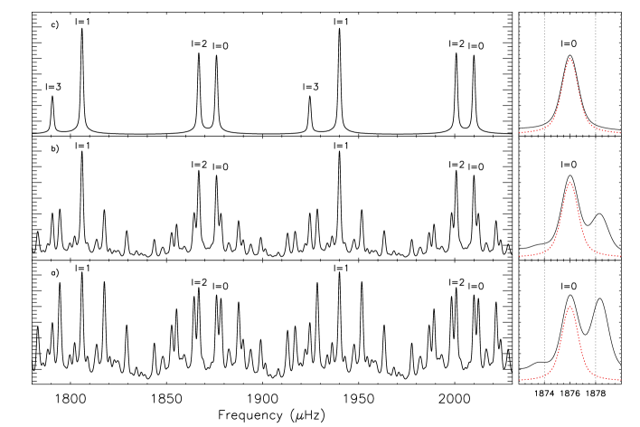
Figure 3: Synthetic amplitude spectra with $\Delta\nu=134.0\,\mu$Hz and $\delta\nu_{02}=9.2\,\mu$Hz (see text), observed from a single (a), from two (b) or from three (c) SONG sites. The rightmost panels display detailed views of a single mode, with dashed red lines representing the undisturbed oscillation mode, black lines representing the modelled amplitude spectrum, which includes contributions from multiple modes as described by the asymptotic relation, and vertical dotted lines showing the spectral region used to calculate the level of contamination. The contamination of the synthetic amplitude spectrum in the bottom panel is below 30%, while it is below 10% in both the center and top panels. The positions of the $l=3$ modes are indicated in the top plot only, for clarity.

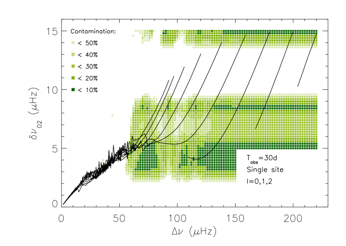
Figure 4: The C-D diagram colour-coded to illustrate amount of overlap between peaks based on each combination of ($\Delta\nu$, $\delta\nu_{02}$), the asymptotic relation and the spectral window function corresponding to observations from a single site. Modes of $l=0,1,2$ have been included when calculating the contamination levels. Dark green areas correspond to combinations of ($\Delta\nu$, $\delta\nu_{02}$) which result in very little overlap, while light-green areas correspond to combinations with significant overlap. White areas correspond to overlaps higher than 50% in amplitude, except in the upper left and lower right corners where no calculations have been done. The stellar models are, as in Fig. 2, from White et al. (2011), again with masses between $0.7-1.5M_{\odot}$ and $Z=0.017$. The width of the frequency peaks has been set to 1.5 $\mu$Hz.

2.2 Constructing the amplitude spectra

To facilitate the discussion of the mode overlap we introduce modified window functions $w_{{\rm mod},k}(\nu)$, where $k=1,2,3$ correspond to the number of nodes. These are defined by modifying the original window functions to reflect peaks whose intrinsic width $2/T\approx 0.77\,\mu$Hz is determined by the assumed length of 30 days of the time series, combined with a Lorentzian with a width determined by the mode lifetime. Here we have assumed a mode lifetime for solar-like oscillations similar to that of the Sun (3 days) – a reasonable simplification for the purpose of studying the impact of the spectral window functions. The relationship between the mode lifetime ($\tau$) and the natural linewidth $\Gamma$ of the mode yields $\Gamma=1/(\pi\tau)\approx 1.23\,\mu$Hz. In practice we constructed $w_{{\rm mod},k}$ by an iterative process, where we smooth the original window function until it has a full width at half maximum (FWHM) of $1.5\,\mu$Hz. This corresponds roughly to adding the intrinsic width of the window function and the natural mode linewidth in quadrature. The peak amplitudes of the modified window functions are kept at 1.0.

When constructing the amplitude spectra, we also use the fact that modes with different $l$-values have different spatial response functions, or sensitivities, for line-of-sight Doppler observations. These are denoted $S_{l}$, and lead to perceived differences in amplitude (e.g., Bedding et al., 1996); the sensitivity of $l=0$ is set to 1.00, $l=1$ to 1.36, $l=2$ to 1.03 and $l=3$ to 0.48.

We now construct the amplitude spectra $a_{k}(\nu)$ by combining the frequencies, $\nu_{n,l}$, with the modified window functions, and taking into account the $l$-dependent sensitivities, $S_{l}$:

$$a_{k}(\nu)=\sum_{n,l}S_{l}\,w_{\rm mod,k}(\nu-\nu_{n,l})\;.$$ (1)

Note that by simply adding the amplitude contributions from each mode we ignore the interference between the modes, depending on their relative phases, which would affect a more realistic combination of the contributions in Fourier space (or the time domain). We expect that this has little effect on the present simplified analysis.

In Fig. 3, we show amplitude spectra for $\Delta\nu=134.0\,\mu$Hz and $\delta\nu_{02}=9.2\,\mu$Hz, as observed from one, two or three SONG telescopes. From these plots, we can see that the artificial peaks introduced by the spectral window function of neighbouring modes can cause the different modes to interfere with each other, as one would expect.

2.3 The contamination of the modes

The degree of overlap (or contamination) is an important parameter in this study. In this part, we examine the amount of contamination arising due to the spectral window function, using the fixed FWHM of 1.5 $\mu$Hz for the mode peaks. In order to evaluate the contamination for a given mode at frequency $\nu$, we determine the signal in the amplitude spectrum, within a 4 $\mu$Hz wide frequency band (see Fig. 3), and compare it to the signal which originates from the undisturbed mode.

From the assumed signal in equation (1) we can, for the different $l$-values of the modes, determine the amount of signal $a_{l,k}$ (including contamination from other modes) in a mode with frequency $\nu_{l}$ as

$$a_{l,k}=\int_{\nu_{1}}^{\nu_{2}}\!a_{k}(\nu)\,\mathrm{d\nu}\;.$$ (2)

Here, $\nu_{1}=\nu_{l}-2\,\mu\rm{Hz}$ and $\nu_{2}=\nu_{l}+2\,\mu\rm{Hz}$. Examples of amplitude spectra $a_{k}(\nu)$ were shown for 1, 2 and 3 sites in Fig. 3. The spectra repeat themselves for each radial order $n$, so for the $l=0$ modes, we may use the mode at $1876\,\mu\rm{Hz}$, for determining the total amount of signal. In this case, $\nu_{1}=1874\,\mu\rm{Hz}$ and $\nu_{2}=1878\,\mu\rm{Hz}$.

In the same way, we can obtain the amount of signal originating only from the mode in question, i.e., the signal that would be inside the frequency band, if the mode were undisturbed. From the central peak in the modified window function $w_{\rm mod,k}(\nu)$ discussed above the amount of signal $w_{l,k}$ for an undisturbed mode is found as

$$w_{l,k}=\int_{-2\,\mu\rm{Hz}}^{+2\,\mu\rm{Hz}}\!S_{l}\,w_{\rm mod,k}(\nu)\,\mathrm{d\nu}\;.$$ (3)

In this way, we obtain for each node configuration, and for each $l$-value, the amount of signal in the combined amplitude spectrum, $a_{l,k}$, and the amount of signal in the undisturbed mode, $w_{l,k}$. We use these values to calculate the amount of contamination as

$$c_{l,k}=(a_{l,k}-w_{l,k})/w_{l,k}\;.$$ (4)

For each node configuration, and for each set of ($\Delta\nu,\delta\nu_{02}$)-values, we first determine the contamination for $l=0,1,2$, leaving out $l=3$, and we assign the highest of these three numbers as the contamination level for that set of parameters. For example, if for one of the node configurations, and for a given combination of $\Delta\nu$ and $\delta\nu_{02}$, the $l=0$ modes are contaminated by 5%, $l=1$ by 15% and $l=2$ by 25%, we assign a contamination level $c_{k}$ for that specific combination of parameters of 25%.

When calculating the contamination, we exclude the contribution from the wings of distant modes; these cause an offset in the spectra, manifesting as a slightly increased background level but having little effect on asteroseismic analysis. This effect is exemplified by the mode depicted in the upper-right panel of Fig. 3; despite some small amount of blending, it is effectively isolated, with a contamination of 0%.

In order to visualize the effect of contamination due to the window function, we compare the $c_{k}$-values to 5 different levels: below 10%, 20%, 30%, 40% and 50% contamination in amplitude, with lower values corresponding to lower degrees of overlap between modes. In the analysis, we cover the parameter space in the C-D diagram with a grid with steps of 2 $\mu$Hz in $\Delta\nu$ and 0.2 $\mu$Hz in $\delta\nu_{02}$. The results of this analysis for 1, 2 and 3 nodes in the network, excluding the lower-amplitude $l=3$ modes from the computations, can be seen in Figs. 4–6.

We then extended the calculations of the mode contamination to include the $l=3$ modes. The results are seen in Figs. 7 and 8. The $l=3$ modes are separated from $l=1$ modes by $\delta\nu_{13}=\frac{5}{3}\delta\nu_{02}$ according to the asymptotic relation. This leads to the exclusion of more cases due to mode-peak overlap.

Figure 5: Same as Fig. 4, but for two SONG telescopes.

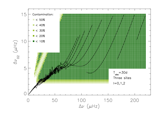
Figure 6: Same as Fig. 4, but for three SONG telescopes.

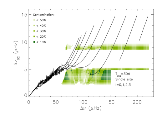
Figure 7: Same as Fig. 4 (a single SONG node), with $l=3$ modes included in the calculation of the mode contamination. Including these modes results in models with $\delta\nu_{02}\sim 7\,\mu$Hz becoming excluded. For these models, $\delta\nu_{13}\sim 11.5\,\mu$Hz (corresponding to 1 d^-1), causing overlap between $l=1$ and $l=3$ modes.

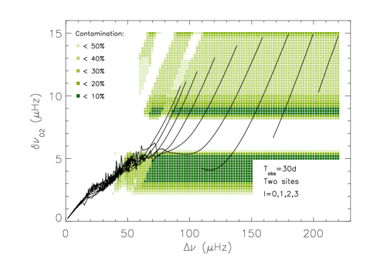
Figure 8: Same as Fig. 7, but for two SONG telescopes.

Figure 9: Colour-coded HR diagram showing the results of our analysis for contamination in the amplitude spectrum of up to 30% for a single SONG node and a time series covering one month, for modes with frequencies near the estimated frequency $\nu_{\rm max}$ of maximum amplitude. Individual models are marked according to the analysis, with green circles marking the models for which seismic analysis is possible, based on our criteria, yellow stars marking models with contamination above 30% due to either the nature of the frequency structure as defined by the asymptotic relation or large mode linewidths, and red diamonds marking models that fail on both the amplitude and overlap requirements. Note that this and the following plots assume a certain noise level per spectrum, and hence do not contain any information on the apparent magnitude of real-sky targets.

2.4 Detecting the seismic signals

We now combine the analysis above with the effects of oscillation mode amplitudes and linewidths on the detection of the asteroseismic signals. In short, the amplitudes must be sufficiently high compared with the noise level for SONG to allow secure detection of the oscillations and the mode linewidths must be narrow enough to allow separation – for some stars, the linewidths can be comparable to or even exceed the small frequency separation, causing significant overlap between modes even for a 100% duty cycle. We base the analysis on estimated parameters near the frequency $\nu_{\rm max}$ of maximum amplitude.

We use the theoretical stellar models to estimate both the oscillation amplitudes and the mode linewidths (i.e., $\Gamma$) across the HR diagram. The mode linewidths depend on effective temperature (Appourchaux et al., 2012) and can therefore vary greatly for different types of stars – indeed, asteroseismology can be extremely difficult for stars with linewidths similar to their frequency separations (e.g., Appourchaux et al., 2008). The mode linewidths are estimated using the relation between $\Gamma$ and the effective temperature, at maximum mode height, from equation (2) and Table 2 in Appourchaux et al. (2012):

$$\Gamma=0.46\,\mu{\rm Hz}+0.75\,\mu{\rm Hz}\left(\frac{T_{\rm eff}}{5777\,{\rm K}}\right)^{15.4}\;.$$ (5)

We extrapolate this relation to include stars with temperatures above $7000\,$K, even though the calibration is based on stars no hotter than $6400\,$K (Appourchaux et al., 2012). By doing so, we slightly overestimate the mode linewidths for these more massive stars relative to those found for F stars in White et al. (2012). We assume that we cannot detect the seismic signal for stars with mode linewidths which are half the value of either the small or large frequency separation. For these stars, the degree of overlap of the mode frequencies compromises the asteroseismic analysis. This is, however, a marginal effect in our analysis.

The overall oscillation amplitudes are estimated for the stellar models by scaling from the solar value, based on equation (17) in Kjeldsen & Bedding (2011):

$$A_{\rm vel}\approx 0.23\,\,{\rm m\,s^{-1}}\times\frac{(L/{\rm L}_{\odot})(\tau_{\rm osc}/\tau_{\rm osc,\odot})^{0.5}}{(M/{\rm M}_{\odot})^{1.5}(T_{\rm eff}/5777{\,\rm K})^{2.25}}\;,$$ (6)

where $\tau_{\rm osc}$ is the mode lifetime.

For this analysis, we compare these amplitudes to the expected noise level for SONG. This depends on the brightness of the star being observed, its spectral type and class, its rotational velocity, and other secondary factors. Here we use a fixed noise value of 2 m s^-1 per spectrum, based on estimates of the properties of the SONG observations and preliminary data from the SONG prototype, with a observing cadence of one datapoint per two minutes, 8 hour long nights per site, and a time series covering 30 d. With this, we expect to achieve noise levels in the amplitude spectra of 4.2 cm s^-1 for a single SONG-node, 3.0 cm s^-1 for two nodes, and 2.4 cm s^-1 for three nodes. We consider the seismic signal detectable if the estimated oscillation amplitude is at least 4 times higher than the predicted noise level. These S/N estimates are valid near the frequency of maximum amplitude for each model, $\nu_{\rm max}$. Figs. 9–12 show the results of this analysis.

3 Results

Figs. 4–8 show the results for the analysis of the impact of window functions on detecting asteroseismic signals for a fixed linewidth of 1.5 $\mu$Hz. From these figures, we can see that stars with $\delta\nu_{02}$ close to 11.57 $\mu$Hz (which corresponds to one cycle per day) will show significant overlap between modes when observed from a single site. The width of the horizontal band centered at 11.57 $\mu$Hz in $\delta\nu_{02}$ depends on the assumed mode linewidth of 1.5 $\mu$Hz; a smaller or larger assumed linewidth means a smaller or larger area being excluded for $\delta\nu_{02}$ values near 11.57 $\mu$Hz.

From Fig. 4, we can see that even for single-site observations, there are areas in the C-D diagram where the mode frequencies will not overlap, despite the significant side-lobes in the spectral window function. This is the case for stars slightly more evolved and less massive than the Sun, among others. This figure also demonstrates the sensitivity of asteroseismology from a single-site to stellar properties: some stars can be targeted from a single site without the analysis being hampered by confusion from overlapping peaks in the amplitude spectrum, while other stars with just slightly different properties cannot.

Figs. 5 and 6 show the results of the analysis for two and three SONG sites. For two sites (Fig. 5), the amplitude spectra of stars with small separations near 11.57 $\mu$Hz will display a 40% overlap between $l=0$ and $l=2$ modes, in good agreement with the corresponding spectral window function in Fig. 1. For three sites, problems with overlapping peaks are eliminated, illustrating the benefits of full temporal coverage. When extending the analysis to include $l=3$ nodes (Figs. 7 and 8), we find that full temporal coverage is required for the detection of $l=3$ modes for most types of stars.

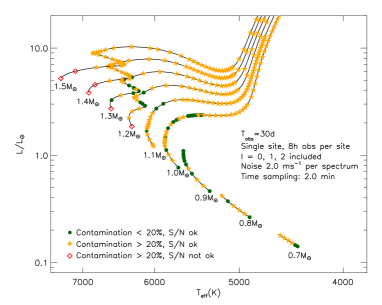
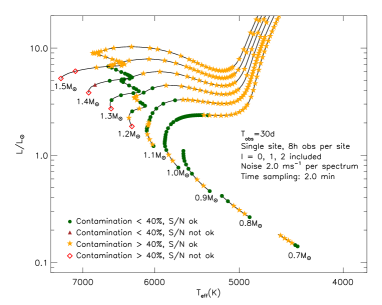
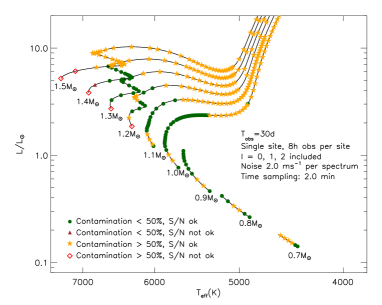
Figure 15: Same as Fig. 4, for a single site including $l=0-2$ and acceptable contamination levels of 10, 20, 40 and 50 per cent.

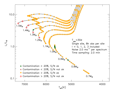
Figure 16: Same as Fig. 4, for a single site including $l=0-3$ and acceptable contamination levels of 10, 20, 40 and 50 per cent.

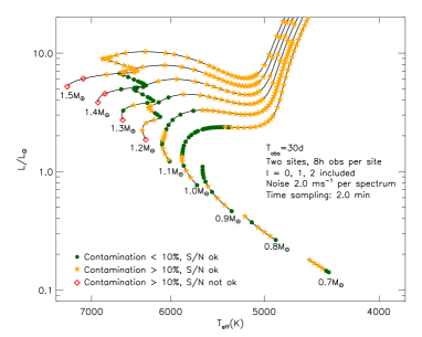
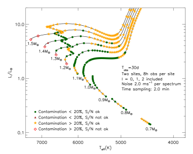
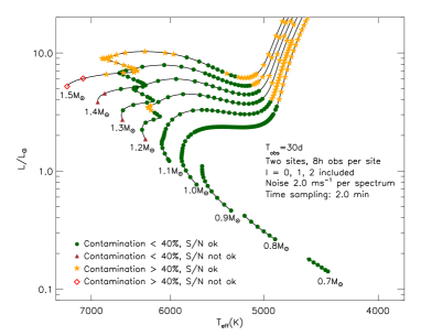
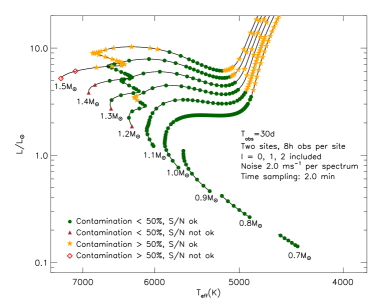
Figure 17: Same as Fig. 4, for two sites including $l=0-2$ and acceptable contamination levels of 10, 20, 40 and 50 per cent.

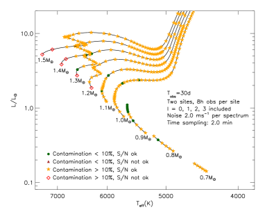
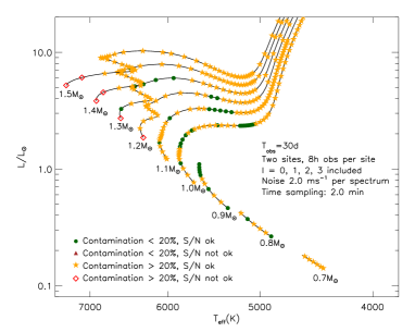
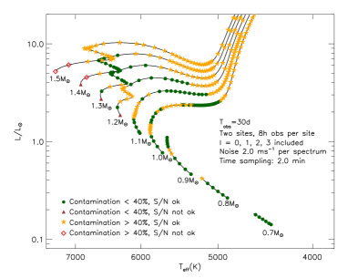
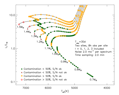
Figure 18: Same as Fig. 4, for two sites including $l=0-3$ and acceptable contamination levels of 10, 20, 40 and 50 per cent.

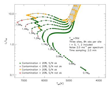
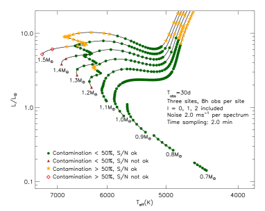
Figure 19: Same as Fig. 4, for three sites including $l=0-2$ and acceptable contamination levels of 10, 20, 40 and 50 per cent.

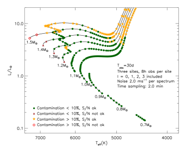
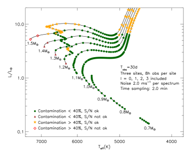
Figure 20: Same as Fig. 4, for three sites including $l=0-3$ and acceptable contamination levels of 10, 20, 40 and 50 per cent.

Figs. 9–12 contain the results of the extended analysis, which includes realistic amplitudes and linewidths. Instead of being plotted in a C-D diagram, the evolutionary tracks are plotted in an HR diagram, showing in which regions of the HR diagram solar-like oscillations can be detected and analysed and in which regions of the diagrams the analysis will be limited by too low signal-to-noise or by mode overlap. The latter can be caused by either a non-optimal combination of frequency splittings and spectral window function or by large mode linewidths. The plots shown here are for a moderate accepted overlap between frequency peaks of up to 30% in amplitude. Similar diagrams can be made for the 4 other thresholds we have used; 10%, 20%, 40% and 50%. These plots are shown in Figs. 15–20.

These plots show that significant, but not all, parts of the HR diagram are excluded for asteroseismic analysis when observing with a single SONG telescope, as well as when observing with two. With three SONG-nodes, seismic analysis is possible across most parts of the HR diagram where solar-like oscillations are expected to occur. For the more massive and hot stars, however, a large mode linewidth combined with relatively low oscillation amplitudes will limit the analysis, even for a fully deployed SONG network.

Fig. 12 is much like Figs. 9–11 but includes the $l=3$ modes, which are lower amplitude than the $l=0,1,2$ modes. Fig. 12 shows the case of two sites; the corresponding figure for three sites is identical to Fig. 11. We do not show the figure for a single site and including $l=3$; in this case, most stellar models are excluded due to mode overlap. This is even the case for two sites (Fig. 12), where the majority of the models are excluded. Adding a third node expands the possibilities considerably, however (see Fig. 11).

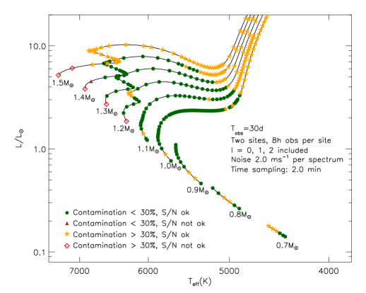
Figure 10: Same as Fig. 9, but for observations with two SONG-nodes. A brown triangle marks a model for which the the signal-to-noise (S/N) of the oscillations is below 4.

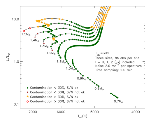
Figure 11: Same as Fig. 9, but for observations with three SONG-nodes. The figure does not change if $l=3$ modes are included in the analysis.

Figure 12: Same as Fig. 10 (observations with two SONG-nodes), but with $l=3$ modes included in the analysis.

4 Discussion

The analysis presented above can not only be used for evaluating target stars for observing solar-like oscillations with a network like SONG, but it can also be used for optimizing observations with such a network.

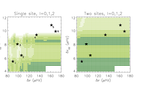
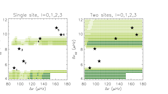
Figure 13: Sample diagrams demonstrating the analysis of individual targets for network of telescopes like SONG. The panels show the contamination level for one and two SONG nodes, without (top) and with (bottom) $l=3$ included for 6 well-studied stars: 1: $\mu$ Ara (Beck et al., 2011); 2: $\alpha$ Cen A (Bedding et al., 2004); 3: HD52265 (Ballot et al., 2011); 4: 18 Sco (Bazot et al., 2012) (and the Sun); 5: $\alpha$ Cen B (Kjeldsen et al., 2005); 6: $\tau$ Ceti (Teixeira et al., 2009). Colour-coding as in Figs. 4–8.

In Fig. 13 we show the level of contamination due to mode overlap for 6 well-observed stars for which the frequency separations of solar-like oscillations have been measured. It is evident that a star similar to $\alpha$ Cen B, which has a small frequency separation $\delta\nu_{02}$ near 11 $\mu$Hz, is not a good target for single site observations aiming at determining the small frequency separation.

From the upper left-hand panel of Fig. 13, we can identify the types of stars for which a single node will be sufficient: those lying below and to the right of 18 Sco, as the dark-green areas indicate regions for which the acoustic spectra of stars will not be significantly affected by overlap between different mode peaks. This complements the information in Fig. 9, which indicates that the amplitudes and mode linewidths of such stars are suitable for study with a single SONG-node for the noise level we have assumed.

The upper right-panel of Fig. 13 represents a network with two nodes. In comparison to a single node, the number of stars for which contamination is a problem is significantly reduced. Consequently, we can envision studying multiple stars at a time with a fully deployed SONG network, with perhaps 4 telescopes distributed on the northern and southern hemispheres, allocating two nodes per target and doubling the rate at which SONG measures the solar-like oscillations in stars.

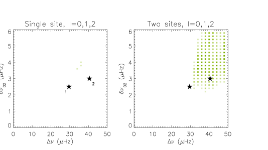
Figure 14: Same as Fig. 13, except that two subgiants for which stellar oscillations have been observed are included: 1: $\beta$ Aql (Corsaro et al., 2012); 2: $\eta$ Boo (Kjeldsen et al., 2003).

Sub-giant stars have comparatively high oscillation amplitudes and are therefore potentially good targets for observations with either one or two SONG nodes. Fig. 14 depicts a subsection of the C-D diagram, where sub-giants are found. It can be seen that for some sub-giants, as for example $\eta$ Boo, the combination of the small and the large frequency separations will allow seismic analysis without significant contamination from the spectral window function, when observing with two SONG nodes. When observing from a single SONG node, the analysis will be strongly affected by effects of the spectral window function.

The results presented in Figs. 9–12 might erroneously suggest that we shall not be able to observe oscillations in red giants with SONG. In fact, the present analysis is based on the asymptotic relation and other assumptions, as described in Sect. 2, which are not entirely relevant for red giants. In particular, the lower frequencies and consequently smaller frequency separations for these stars mean that observations longer than the 30 d assumed here will be needed to avoid confusion. A separate analysis will be required to evaluate the potential of SONG for the study of red giants.

5 Conclusions

The methods presented here demonstrate an approach for evaluating targets for measuring solar-like oscillations spectroscopically using either a single telescope or a network of telescopes. While the SONG network is the inspiration for this analysis, it is generalizable to any single or multi-site campaign with a similar goal in mind.

We have shown that under the assumptions we have made, for certain targets, one or two SONG telescopes will be sufficient to observe solar-like oscillations without the subsequent seismic analysis being hampered by overlapping mode peaks in the amplitude spectrum. However, it is important to remember that the specific science goals of an individual project define the acceptable level of contamination for an amplitude spectrum or what $S/N$-level is required – or is even possible. It is not the goal of this paper to recommend or rule out potential solar-like targets for SONG. This analysis is intended to assess the benefit of additional nodes in the SONG network and to develop a tool for future evaluations of specific targets for SONG, taking information like target brightness, rotational velocity and position in the HR diagram and contributing to the target selection process and scheduling for SONG.

Based on our analysis, we conclude that certain targets will require only one or two SONG nodes to enable the detection of solar-like oscillations despite contamination of the amplitude spectrum due to the window function. However, the detection of solar-like $l=3$ modes requires full network coverage for most of that part of the HR diagram where we expect stars to exhibit solar-like oscillations. Given that detection of $l=3$ modes is an important science driver for SONG – and one of the factors that will push the analysis of solar-like stars beyond what can be reached with the Kepler mission – we conclude that, while the two SONG nodes currently under construction will represent an important advance for ground-based asteroseismology, they are not sufficient to fulfill the ultimate science goals of SONG.

References

- Appourchaux et al. (2008) Appourchaux T., et al. 2008, A&A 488, 705
- Appourchaux et al. (2012) Appourchaux T., et al. 2012, A&A 537, A134
- Ballot et al. (2011) Ballot J., et al. 2011, A&A 530, A97
- Bazot et al. (2012) Bazot M., et al. 2012, A&A 544, A106
- Beck et al. (2011) Beck P. G., et al. 2011, Science 332, 205
- Bedding et al. (1996) Bedding T. R., Kjeldsen H., Reetz J., Barbuy B. 1996, MNRAS 280, 1155
- Bedding et al. (2004) Bedding T. R., Kjeldsen H., Butler R. P., McCarthy C., Marcy G. W., O’Toole S. J., Tinney C. G., Wright J. T. 2004, ApJ 614, 380
- Bouchy et al. (2005) Bouchy F., Bazot M., Santos N. C., Vauclair S., Sosnowska D. 2005, A&A 440, 609
- Chaplin et al. (2011) Chaplin W. J., et al. 2011, Science 332, 213
- Christensen-Dalsgaard (1984) Christensen-Dalsgaard J. 1984, in Mangeney, A., Praderie, F., eds, Space Research Prospects in Stellar Activity and Variability. Paris Observatory Press, Paris, p. 11
- Christensen-Dalsgaard (1988) Christensen-Dalsgaard J. 1988, in Christensen-Dalsgaard J., Frandsen S., eds, Proc. IAU Symp. 123, Advances in helio- and asteroseismology. Reidel, Dordrecht, p. 295
- Christensen-Dalsgaard (2012) Christensen-Dalsgaard J. 2012, AfrSk, 16, 74
- Christensen-Dalsgaard & Thompson (1997) Christensen-Dalsgaard J., Thompson M. J. 1997, MNRAS, 284, 527
- Corsaro et al. (2012) Corsaro E., Grundahl F., Leccia S., Bonanno A., Kjeldsen H., Paternò 2012, A&A 537, A9
- Cunha & Metcalfe (2007) Cunha M. S., Metcalfe T. S. 2007, ApJ, 666, 413
- Gilliland et al. (2010) Gilliland R. L., et al. 2010, PASP 122, 131
- Gough (1986) Gough D. O. 1986, in Osaki, Y., ed., Hydrodynamic and magnetodynamic problems in the Sun and stars. University Tokyo Press, Tokyo, p. 117
- Gough (1990) Gough D. O., 1990, in Osaki, Y. & Shibahashi, H., eds, Progress of seismology of the sun and stars, Lecture Notes in Physics, vol. 367, Springer, Berlin, p. 283
- Grundahl et al. (2006) Grundahl F., Kjeldsen H., Frandsen S., Andersen M., Bedding T. R., Arentoft T., Christensen-Dalsgaard J. 2006, Mem. Soc. Astron. Ital. 77, 458
- Grundahl et al. (2009) Grundahl F., Christensen-Dalsgaard J., Arentoft T., Frandsen S., Kjeldsen H., Jørgensen U. G., Kjærgaard P. 2009, Communications in Asteroseismology, 158, 345
- Houdek & Gough (2007) Houdek G., Gough D. O., 2007, MNRAS 375, 861
- Kjeldsen & Bedding (2011) Kjeldsen H., Bedding, T. R., 2011, A&A 529, L8
- Kjeldsen et al. (2003) Kjeldsen H., et al. 2003, AJ 126, 1483
- Kjeldsen et al. (2005) Kjeldsen H., et al. 2005, ApJ 635, 1281
- Tassoul (1980) Tassoul M., 1980, ApJS 43, 469
- Teixeira et al. (2009) Teixeira T. C., et al. 2009, A&A 494, 237
- Vandakurov (1967) Vandakurov Y. V. 1967, AZh. 44, 786
- Ulrich (1986) Ulrich R. K. 1986, ApJ, 306, L37
- White et al. (2011) White T. R., Bedding T. R., Stello D., Christensen-Dalsgaard J., Huber D., Kjeldsen H. 2011, ApJ 743, 13
- White et al. (2012) White T. R., et al. 2012, ApJ 751, L36