Half-integrality, LP-branching and FPT Algorithms

Abstract

A recent trend in parameterized algorithms is the application of polytope tools (specifically, LP-branching) to FPT algorithms (e.g., Cygan et al., 2011; Narayanaswamy et al., 2012). Though the list of work in this direction is short, the results are already interesting, yielding significant speedups for a range of important problems. However, the existing approaches require the underlying polytope to have very restrictive properties, including half-integrality and Nemhauser-Trotter-style persistence properties. To date, these properties are essentially known to hold only for two classes of polytopes, covering the cases of Vertex Cover (Nemhauser and Trotter, 1975) and Node Multiway Cut (Garg et al., 1994).

Taking a slightly different approach, we view half-integrality as a discrete relaxation of a problem, e.g., a relaxation of the search space from $\{0,1\}^{V}$ to $\{0,{\nicefrac{{1}}{{2}}},1\}^{V}$ such that the new problem admits a polynomial-time exact solution. Using tools from CSP (in particular Thapper and Živný, 2012) to study the existence of such relaxations, we are able to provide a much broader class of half-integral polytopes with the required properties.

Our results unify and significantly extend the previously known cases. In addition to the new insight into problems with half-integral relaxations, our results yield a range of new and improved FPT algorithms, including an $O^{*}(|\Sigma|^{2k})$-time algorithm for node-deletion Unique Label Cover with label set $\Sigma$ (improving the previous bound of $O^{*}(|\Sigma|^{O(k^{2}\log k)})$ due to Chitnis et al., 2012) and an $O^{*}(4^{k})$-time algorithm for Group Feedback Vertex Set, including the setting where the group is only given by oracle access (improving on the previous bound of $O^{*}(2^{O(k\log k)})$ due to Cygan et al., 2012). The latter bound is optimal under the Exponential Time Hypothesis. The latter result also implies the first single-exponential time FPT algorithm for Subset Feedback Vertex Set, answering an open question of Cygan et al. (2012). Additionally, we propose a network flow-based approach to solve some cases of the relaxation problem. This gives the first linear-time FPT algorithm to edge-deletion Unique Label Cover.

Interestingly, despite the half-integrality, our result do not imply any approximation results (as may be expected, given the Unique Games-hardness of the covered problems).

1 Introduction

Polytope methods, and methods related to linear and integer programming in general, have been hugely successful in combinatorial optimisation, both for deriving exact polynomial-time results and for purposes of approximation (see, e.g., the book of Schrijver [50]). However, the methods have seen less application for questions of getting faster exact (i.e., non-approximate) solutions to NP-hard problems, at least from a theoretical perspective. (Industrial mixed integer programming-solvers such as CPLEX, though frequently efficient, are not our concern here since usually, no non-trivial performance guarantees are known.)

A few such applications have emerged in recent years in the field of parameterized complexity; specifically, two sets of problems – Node Multiway Cut [18] and problems related to Vertex Cover [41, 40] – have been shown to be FPT parameterized by the above LP parameter, i.e., given an instance of one of these problems, it can be decided in $O^{*}(4^{k})$ time whether there is a solution that is at most $k$ points more expensive than the LP-optimum. In the former case, due to the integrality gap of the Multiway Cut LP [23], this results in an $O^{*}(2^{k})$-time FPT algorithm for the natural parameterization of the problem, improving on previous results of $O^{*}(4^{k})$; in the latter case, through parameter-preserving problem reductions, the result is improved FPT algorithms for a range of problems (e.g., problems expressible in Almost 2-SAT, a.k.a., 2-CNF deletion).

However, despite the promise of the approach (and the programmatic view taken in the latter set of papers [41, 40]), we still know only few such applications. (Also note that if $k$ is taken as the above “gap” parameter, then in general it would be NP-hard to decide whether $k=0$.) Furthermore, an inspection of the tools used reveal that the methods are quite similar, and very specific; it is a matter of FPT applications of the half-integrality results of Nemhauser and Trotter [42] in the latter case, and similar half-integrality results for Node Multiway Cut in the former case, as shown by Garg et al. [23] and refined for FPT purposes by Guillemot [24] and Cygan et al. [18]. Therefore, a good first step towards a better understanding of the power of LP-relaxations for FPT problems (or vice versa, e.g., to further the parameterized study of mixed integer programming) seems to be to consider specifically the property of half-integrality.

1.1 Integral and half-integral polytopes

Compared to our knowledge about integral polytopes (e.g., connections to totally unimodular matrices and the notion of total dual integrality), our knowledge of half-integrality seems rather more spotty. It seems that most of what is available can be enumerated as a few quick examples, e.g., the above-mentioned cases of Vertex Cover [42] and Node Multiway Cut [23]; Hochbaum’s IP2 programs [25]; and a few related cases, such as the continuous relaxation for Submodular Vertex Cover [30]. Of these, probably the most ambitious study of half-integrality is the work of Hochbaum [25], where a general IP of a certain restricted form is shown to admit half-integral solutions. Still, of the applications mentioned in [25], most if not all (e.g., all applications with a Boolean domain) can be covered by a simple reduction to Almost 2-SAT. One should also mention Kolmogorov [37]; see below.

One important note is that half-integrality is more specific than having an integrality gap of $2$. While the latter clearly implies the same approximation result, half-integrality imposes much more structure on the solutions of a problem (as seen, e.g., by the FPT applications above and in the rest of this paper). Examples of LP-relaxations which are 2-approximate but not half-integral would include Multicut in Trees [22] and Feedback Vertex Set [12]; see also results achieved via iterative rounding [32, 20], e.g., for Steiner Tree. In the present paper, we ignore such results, and focus on the topic of half-integrality.

In this work, to discover half-integral relaxations, we take a slightly different approach to the problem from most of the above, inspired rather by the work of Kolmogorov [37]. In essence, we start from the observation that a half-integral relaxation, unlike a generic 2-approximate LP-relaxation, actually defines a polynomial-time solvable problem on a discrete search space of $\{0,{\nicefrac{{1}}{{2}}},1\}^{n}$. Thus, we argue that the search for half-integral relaxations, and even for half-integral polytopes, would benefit from the application of tools designed to characterise exactly solvable problems, e.g., tools from the study of constraint satisfaction problems.

1.2 CSPs and LP-relaxations

Constraint satisfaction problems (CSPs) make for a general setting in which the complexity of various problems can be studied in a systematic way. In the most common setting, one studies generalisations of SAT: Given a (one-time fixed) set $\Gamma$ of relation types, what is the complexity of deciding the satisfiability of a formula which consists of a conjunction of applications of relations $R\in\Gamma$? For example, by fixing the domain to be Boolean, and letting $\Gamma$ contain all 3-clauses, one would encode the problem 3-SAT.

For optimisation problems, a generalisation of valued CSPs (VCSPs) has been proposed. Roughly, in this setting, instead of using relations, one fixes a set $\mathcal{F}$ of cost functions; an instance consists of a set of applications of functions $f_{i}\in\mathcal{F}$, and the task is to minimise (or maximise) the sum of the values of the functions in the input. One particular case (which has been studied extensively in approximation) is when the cost functions all take values $0$ and $1$ only, thus encoding a “soft version” of a constraint; e.g., $f(u,v)=[u=v=0]$ (taking cost $1$ if $u=v=0$, cost $0$ otherwise) would be the soft version of a constraint $(u\lor v)$. (In some approximation literature the maximisation version of VCSP for such soft versions of constraints is taken as the definition of the CSP problem itself.) Again, the interest is in identifying which sets $\mathcal{F}$ of cost functions imply polynomial-time solvable versus NP-hard problems, or more closely what approximation properties the resulting CSP would have.

The use of various relaxations has been of critical importance to the solutions for these problems. For approximation, the best results have been attained using SDP relaxations, and Raghavendra [47] showed that assuming the unique games conjecture [36], a particular SDP relaxation achieves the optimal approximation ratio for every Max CSP problem. However, for the question of whether finding an exact solution is in P or NP-hard, it turns out, somewhat surprisingly, that it suffices to use a simple LP-relaxation (known as the basic LP, being essentially a simpler version of the appropriate level in the Sherali-Adams hierarchy).

To be precise, it follows from a sequence of work by Thapper and Živný and by Kolmogorov [51, 38, 52] that for every set of finite-valued cost functions $\mathcal{F}$, either the basic LP solves the resulting VCSP exactly, or the VCSP problem is APX-hard. Thus, despite our excursion into CSPs, the connection to LP-relaxations and polytope theory remains, in particular as the LP-relaxation remains the only known method of solving the problem for several of the covered problem classes.

Our application of this framework takes the following shape. Assume an NP-hard VCSP problem, defined by a class of cost functions $\mathcal{F}$ on a finite domain $D$ (i.e., the search space of the problem is $D^{n}$). If our problem has a half-integral LP-relaxation, then there should also exist a class $\mathcal{F}^{\prime}$ of “relaxed” versions of the cost functions, working in a search space $(D^{\prime})^{n}$ (e.g., $D^{\prime}$ would be $D$ extended by the half-integral values), such that $\mathcal{F}^{\prime}$ defines a polynomial-time solvable problem. We call such a class $\mathcal{F}^{\prime}$ a discrete relaxation of the original problem, and refer to values from the original domain $D$ (e.g., $\{0,1\}$) as integral values, and values from $D^{\prime}\setminus D$ (e.g., $\nicefrac{{1}}{{2}}$) as relaxed values. (We also need some technical requirements; see Section 3.)

Assuming that such a discrete relaxation $\mathcal{F}^{\prime}$ is found, we may then use an algorithm, akin to the LP-branching algorithms of [18, 41, 40], to solve our original problem in FPT time, parameterized by the size of the relaxation gap. The connection to half-integrality lies in the basic LP of the relaxed class $\mathcal{F}^{\prime}$; in our examples, $\mathcal{F}^{\prime}$ is a half-integral relaxation of $\mathcal{F}$, and the basic LP can be used to construct a simpler LP-relaxation for the original problem, which then is found to be half-integral.

1.3 Our results

We show that many known half-integrality results, and several new ones, can be explained by applying the above framework using the class of $k$-submodular functions as discrete relaxations. This includes the above cases of (Submodular Cost) Vertex Cover, Almost 2-SAT, and Node Multiway Cut, as well as a further generalisation of the first two called Bisubmodular Cost 2-SAT. In addition, we construct new, possibly unexpected half-integral LP-relaxations for the Group Feedback Vertex Set and Unique Label Cover problems, leading to significantly improved FPT algorithms; see below.

The framework immediately implies an integral LP-formulation of the half-integral relaxations of the above-mentioned problems (i.e., an integral polytope over a larger set of variables); however, the resulting formulation has for many problems an inconveniently large dimension, preventing it to be used in full generality. To work around this problem, we construct an alternative, half-integral LP-relaxation with fewer variables, inspired by the basic LP and the construction in [23].

Unique Label Cover is the problem which lies at the heart of the unique games conjecture [36], which is of central importance to the field of approximation algorithms. Previous work by Chitnis et al. [11] gave an $O^{*}(|\Sigma|^{O(p^{2}\log p)})$-time FPT algorithm for the problem using a highly involved probabilistic approach (here, $\Sigma$ is the label set, and $p$ is the solution cost). Via our new LP-relaxation, we solve the problem in time $O^{*}(|\Sigma|^{2p})$, for both the edge- and vertex-deletion versions; furthermore, our result is deterministic.

Group Feedback Vertex Set (GFVS) is a powerful generalisation of Feedback Vertex Set and Odd Cycle Transversal; we refer to Section 5 and the cited literature for details. The FPT study of this problem was initiated by Guillemot [24]; Cygan et al. [17] showed that the problem is FPT in a very general form (technically, when the input provides only black-box oracle access to the group), with a running time of $O^{*}(2^{O(k\log k)})$. They note that in this general form, GFVS subsumes Subset Feedback Vertex Set, for which an $O^{*}(2^{O(k\log k)})$-time algorithm was previously given [19]. They note that their running time seems difficult to improve with their methods, and asks whether their result could be optimal under ETH (the Exponential-Time Hypothesis [28]).

Using the above-mentioned LP-relaxation, we would get an algorithm only for the case that the group is given in explicit form (i.e., not as an oracle); in particular, we would have to limit ourselves to groups of polynomial size. However, many useful cases of GFVS (including the reductions from Feedback Vertex Set and Subset Feedback Vertex Set) use exponential-sized groups, and hence require the oracle form. To cover this case, we provide an alternative LP-relaxation of the problem, which has an exponential number of constraints, but which can be solved using a separation oracle. This implies an $O^{*}(4^{k})$-time FPT algorithm for Group Feedback Vertex Set with group given via oracle access, providing the first single-exponential FPT algorithms for GFVS and for Subset Feedback Vertex Set, hence answering the questions of Cygan et al. [17]. The new running times are optimal under ETH.

1.3.1 Linear-time FPT algorithms

As we have described above, the LP-branching based on discrete relaxations is a promising approach to establish FPT algorithms and to reduce $f(k)$ part of the running time. However, its $\mathrm{poly}(n)$ part is not so small since it relies on linear programming to solve the relaxations. Reducing the $\mathrm{poly}(n)$ part is also an important task in FPT algorithms. Especially, there have been many researches on FPT algorithms whose $\mathrm{poly}(n)$ part is only linear (linear-time FPT), e.g., Tree-Width [2] and Crossing Number [35]. Very recently, linear-time FPT algorithms for Almost 2-SAT have been developed independently by Ramanujan and Saurabh [48], and Iwata, Oka and Yoshida [31]. The idea of the algorithm by Iwata et al. is to reduce the computation of LP relaxation to a minimum cut, and actually, this approach works for solving several of our relaxation problems. This approach generalise the linear-time FPT algorithm for Almost 2-SAT and gives the first linear-time FPT algorithm for edge-deletion Unique Label Cover that runs in $O(|\Sigma|^{2p}m)$ time. Thus the LP-branching based on discrete relaxations has a potential to reduce both $f(k)$ and $\mathrm{poly}(n)$ simultaneously.

1.4 Related work

Hochbaum [25] gave a general framework for half-integral relaxations of certain optimisation problems (as discussed above), via a form of integer program called IP2 (which in turn is solved via relaxation to a polynomial-time solvable problem class called monotone IP2). Without going into too much technical detail, we note that monotone IP2s are covered in a VCSP framework by problems submodular on a chain [34, 29, 49], and that the Boolean-domain case of IP2 reduces directly to Almost 2-SAT, a.k.a. 2-CNF Deletion. However, we have not reconstructed a direct VCSP interpretation of the full case of half-integral IP2. Hochbaum [25] asks in her paper whether the problems of Node Multiway Cut and Multicut on Trees can be brought into her framework; the problem of Multicut on Trees remains open to us.

Kolmogorov [37] gave close connections between functions with half-integral minima and bisubmodular functions, in particular showing that bisubmodular functions correspond (in a certain sense) to a class of (continuous-domain) functions referred to as totally half-integral. See Section 3.1 for more details.

Submodular and bisubmodular functions also occur as rank functions of, respectively, matroids [43] and delta-matroids [3]; there are also connections to polytope theory (e.g., [8]). Similar, but less well-explored connections exist for $k$-submodular functions; see the theory of multi-matroids [4, 5, 7, 6], and the polytope connection given by Huber and Kolmogorov [26].

Group-labelled graphs (as in Group Feedback Vertex Set) and bijection-labelled graphs (as in Unique Label Cover) have been explored from a graph-theory perspective, in particular with respect to path-packing; see [13, 14, 27] and [44, 45].

2 Preliminaries

2.1 Valued CSPs

Let $D$ be a fixed, finite domain. A cost function on $D$ (of arity $r$) is a function $f:D^{r}\rightarrow\mathbb{R}$. A valued constraint is an application $f(v_{1},\ldots,v_{r})$ of a cost function $f:D^{r}\rightarrow\mathbb{R}$ to a tuple of variables $(v_{1},\ldots,v_{r})$. For simplicity, we disallow repeated variables in constraints; this will make no difference for our results but will simplify some notation. A valued CSP instance (VCSP instance) is defined by a set $V$ of variables and a list of valued constraints $f_{1}(v_{1,1},\ldots,v_{1,r_{1}}),\ldots,f_{m}(v_{m,1},\ldots,v_{m,r_{m}})$, where $v_{i,j}\in V$ for each $i,j$; given an assignment $\phi:V\rightarrow D$ and a VCSP instance $I$, we define the total cost of $\phi$ for $I$ as $f_{I}(\phi)=\sum_{i=1}^{m}f_{i}(\phi(v_{i,1}),\ldots,\phi(v_{i,r_{i}})).$ Given a (not necessarily finite) set $\mathcal{F}$ of cost functions on domain $D$, the valued CSP problem VCSP$(\mathcal{F})$ is the following problem: given a VCSP instance $I$ on variable set $V$, where every cost function $f_{i}$ is contained in $\mathcal{F}$, and a number $k$, find an assignment $\phi:V\rightarrow D$ such that $f_{I}(\phi)\leq k$.

A crisp constraint is one which cannot be broken (e.g., of infinite or prohibitive cost). Given a relation $R$, let the soft version of $R$ denote the valued constraint such that $f(X)=0$ if $R(X)$ holds, and $f(X)=1$ otherwise.

We will be most interested in the class of $k$-submodular functions, defined as follows. Fix a domain $D=\{0,1,\ldots,k\}$, and let $\sqcap,\sqcup$ be symmetric, idempotent operations such that $0\sqcap x=0$ for any $x\in D$; $0\sqcup x=x$ for any $x\in D$; and $x\sqcap y=x\sqcup y=0$ for any $x,y\in D\setminus\{0\}$ with $x\neq y$. A function $f:D^{r}\rightarrow\mathbb{R}$ is $k$-submodular if $f(X)+f(Y)\geq f(X\sqcap Y)+f(X\sqcup Y)$ for all $X,Y\in D^{r}$. The case $k=2$ is referred to as bisubmodular functions.

2.2 The basic LP relaxation

Since it is fundamental to our paper, let us explicitly define the LP which lies behind all the above tractability results. Let $\mathcal{F}$ be a finite set of cost functions over a domain $D$, and let $I$ be an instance of VCSP$(\mathcal{F})$ on variable set $V=\{v_{1},\ldots,v_{n}\}$ and with valued constraints $f_{i}(v_{i,1},\ldots,v_{i,r_{i}})$, $1\leq i\leq m$. The basic LP relaxation (BLP) of $I$ is defined as follows. (The definition given in [51] is slightly different, but can easily be verified to be equivalent to the formulation below for our case.) Introduce variables $\mu_{v=d}$ for every $v\in V$ and $d\in D$, and $\lambda_{f_{i},\sigma}$ for every valued constraint $f_{i}$ in $I$ and every $\sigma\in D^{r_{i}}$. The (BLP) is defined as follows.

$$\min \sum_{i=1}^{m}\sum_{\sigma\in D^{r_{i}}}f_{i}(\sigma(1),\ldots,\sigma(r_{i}))\cdot\lambda_{f_{i},\sigma}$$

$$\mathrm{s.t.} \sum_{d\in D}\mu_{v=d}=1 \forall v\in V$$

$$\sum_{\sigma\in D^{r_{i}}:\sigma(j)=d}\lambda_{f_{i},\sigma}=\mu_{v=d} \forall 1\leq i\leq m,1\leq j\leq r_{i},d\in D,v=v_{i,j}$$

$$0\leq\lambda_{f_{i},\sigma},\mu_{v=d}\leq 1$$

Note that the size of the LP depends badly on function arity, e.g., we introduce $|D|^{r}$ variables for a single $r$-ary valued constraint $f$. However for every finite set of functions, as required above, this arity is bounded and the LP is of polynomial size. We will later in the paper define smaller, equivalent LP-relaxations for particular problem classes.

To reiterate, it is a consequence of [51] that if $\mathcal{F}$ is a set of $k$-submodular functions, then the above LP solve VCSP($\mathcal{F}$) precisely.

2.3 Polymorphisms and fractional polymorphisms

A key tool in the characterisation of CSP complexity is the algebraic method. For a domain $D$, an operation $h:D^{t}\rightarrow D$, and a list of tuples $A_{1},\ldots,A_{t}\in D^{\ell}$, define $h(A_{1},\ldots,A_{t})\in D^{\ell}$ as the result of applying $h$ column-wise to the tuples, i.e., if $A(j)$ denotes the $j$-th entry of a tuple $A$, we let $h(A_{1},\ldots,A_{t})$ be the tuple $T\in D^{\ell}$ such that $T(i)=h(A_{1}(i),\ldots,A_{t}(i))$. Given a relation $R\subseteq D^{r}$, a polymorphism of $R$ is an operation $h:D^{t}\rightarrow D$ such that for any tuples $A_{1},\ldots,A_{t}\in R$, we have $h(A_{1},\ldots,A_{t})\in R$ (i.e., the relation $R$ is closed under the operation of applying $h$ column-wise on any set of $t$ tuples in $R$). For a set of relations $\Gamma$, we say that $\Gamma$ has a polymorphism $h$ if $h$ is a polymorphism of every $R\in\Gamma$. It is known that the complexity of classical (feasibility) CSP$(\Gamma)$ is characterised by the set of polymorphisms of the allowed relation types $\Gamma$, however, no complete dichotomy is known for this question.

We will need only the following notion: A majority polymorphism is a polymorphism $h:D^{3}\rightarrow D$ such that $h(x,x,y)=h(x,y,x)=h(y,x,x)=x$ for any $x,y\in D$. It is known that for any set of relations $\Gamma$ with a majority polymorphism, the solution set for any formula over $\Gamma$ can be described using only binary relations (derivable from $\Gamma$); see [33].

For valued constraints, the notions must be expanded to fractional polymorphisms; see [51, 52] for definitions, and for an exact characterisation of the VCSP dichotomy results. For this paper, we will be content with a simpler notion. Let $f:D^{r}\rightarrow\mathbb{R}$ be a cost function. A binary multimorphism of $f$ is a pair of operations $\langle h_{1},h_{2}\rangle:D^{2}\rightarrow D$ such that for any $A,B\in D^{r}$, we have $f(A)+f(B)\geq f(h_{1}(A,B))+f(h_{2}(A,B))$. Similarly to above, $\langle h_{1},h_{2}\rangle$ is a multimorphism of a set $\mathcal{F}$ of cost functions if it is a multimorphism of every $f\in\mathcal{F}$. The prime example would be the submodular functions, which are defined on domain $D=\{0,1\}$ by the multimorphism $\langle\cap,\cup\rangle$ (i.e., $f(X)+f(Y)\geq f(X\cap Y)+f(X\cup Y)$); it is well known that submodular functions can be minimised efficiently (e.g., [29, 49]). Other examples of function classes $\mathcal{F}$ which imply that VCSP$(\mathcal{F})$ is tractable include (among other cases) functions submodular on an arbitrary lattice, defined as having the multimorphism $\langle\lor,\land\rangle$, and functions (weakly or strongly) submodular on a tree; see [51] for details.

3 Discrete Relaxations and FPT Branching

We now describe our approach more precisely.

Definition 1.

Let $f:D^{r}\rightarrow\mathbb{R}$ be a finite-valued cost function. A discrete relaxation of $f$ on domain $D^{\prime}\supset D$ is a function $f^{\prime}:(D^{\prime})^{r}\rightarrow\mathbb{R}$, such that (i) $\min_{\bar{x}\in(D^{\prime})^{r}}f^{\prime}(\bar{x})=\min_{\bar{x}\in D^{r}}f(\bar{x})$, and (ii) $f(\bar{x})=f^{\prime}(\bar{x})$ for every $\bar{x}\in D^{r}$. A discrete relaxation of a set of cost functions $\mathcal{F}=\{f_{1},\ldots,f_{t}\}$ is a set of cost functions $\mathcal{F}^{\prime}=\{f_{1}^{\prime},\ldots,f_{t}^{\prime}\}$ on a domain $D^{\prime}\supset D$, such that $f_{i}^{\prime}$ is a discrete relaxation of $f_{i}$ for each $i\in[t]$. Finally, given an instance $I$ of VCSP$(\mathcal{F})$, the relaxed instance $I^{\prime}$ of VCSP$(\mathcal{F}^{\prime})$ is created by replacing every cost function $f_{i}$ in $I$ by its corresponding relaxation $f_{i}^{\prime}$. The (additive) relaxation gap of $I$ is OPT$(I)$-OPT$(I^{\prime})$.

Note that we can have $\mathrm{OPT}(I)>\mathrm{OPT}(I^{\prime})$ despite every individual cost function $f_{i}$ having an identical minimum (e.g., if setting $v=d^{\prime}$ for every variable $v$ minimises every constraint, for some $d^{\prime}\in D^{\prime}\setminus D$). If $\mathcal{F}$ is integer-valued, let the scaling factor of the relaxation $\mathcal{F}^{\prime}$ be the smallest rational $c$ such that $c\cdot f_{i}^{\prime}$ is integral for every $f_{i}^{\prime}\in\mathcal{F}^{\prime}$. In this case, we say that $\mathcal{F}^{\prime}$ is a $c$-relaxation of $\mathcal{F}$ (note that this does not necessarily imply that $I^{\prime}$ is an approximation).

Definition 2.

Let $\mathcal{F}$ be a set of cost functions on a domain $D$, with a discrete relaxation $\mathcal{F}^{\prime}$ on domain $D^{\prime}$. We refer to the values of $D$ as the original values, and $D^{\prime}\setminus D$ as the relaxed values. In an assignment $\phi:V\rightarrow D^{\prime}$, we say that a variable $v\in V$ is integral in $\phi$ if $\phi(v)\in D$; otherwise, $v$ is relaxed in $\phi$. An assignment $\phi$ is integral if it uses only original values, i.e., if every variable $v\in V$ is integral in $\phi$. Borrowing a term from Kolmogorov [37], we say that the relaxation is persistent if, for any optimal assignment $\phi^{*}$ of a relaxed instance $I^{\prime}$, there is an optimal integral assignment $\phi$ that agrees with $\phi^{*}$ on the latter’s integral values (i.e., if $\phi^{*}(x)$ is integral, then $\phi(x)=\phi^{*}(x)$).

As a slight technical point, note that persistence is a function of the division of the domain $D^{\prime}$ into integral and relaxed parts, and does not explicitly require a reference to an original function on a domain $D$ being relaxed. In our main case, we will deal with functions on a domain of $D=\{1,\ldots,k\}$, which have relaxations on a domain $D^{\prime}=\{0,\ldots,k\}$ which are $k$-submodular. Thus, we will have a single relaxed domain value of $0$.

To illustrate the notions, we show the application to Vertex Cover. Consider the Boolean domain $D=\{0,1\}$. Let $f_{\lor}$ be defined by $f_{\lor}(0,0)=1$, and $f_{\lor}(x,y)=0$ otherwise (i.e., $f_{\lor}$ is the soft version of the relation $(x\lor y)$), and let $f_{0}(x)=x$ (corresponding to the soft version of requiring $x=0$). Then VCSP$(f_{\lor},f_{0})$ is NP-hard, as it encodes Vertex Cover when $f_{\lor}$ is treated as a crisp constraint. On the other hand, let $D^{\prime}=\{0,{\nicefrac{{1}}{{2}}},1\}$, and define the relaxations $f^{\prime}_{\lor}(x,y)=\max(0,1-x-y)$ and $f_{0}^{\prime}(x)=x$. Then this is a discrete relaxation of the original problem, which furthermore is a persistent 2-relaxation and can be solved in polynomial time, as it corresponds to the classical LP-relaxation of Vertex Cover (see Nemhauser and Trotter [42]). Furthermore, the relaxed functions are bisubmodular if $D^{\prime}$ is renamed as $(0,{\nicefrac{{1}}{{2}}},1)\mapsto(1,0,2)$.

This example also roughly illustrates the connections between tractable discrete relaxations and half-integrality. From [51] we have that for every tractable set of cost functions $\mathcal{F}$, and every instance $I$ of VCSP$(\mathcal{F})$, the optimum of the basic LP relaxation (BLP) coincides with OPT$(I)$. Since the results of [51] support weighted functions (e.g., an input of $w_{i}\cdot f_{i}(\cdot)$ rather than just $f_{i}(\cdot)$), and since such weights only occur in the cost function of the LP, it must be that every vertex of the LP is integral, i.e., that (BLP) is an integral LP. Now, rather than a half-integral LP, this is an integral LP on a different, larger set of variables, however, in the cases considered in this paper (bisubmodular and $k$-submodular functions), we will see that such a larger LP can (at least in specific cases) be mapped down to a half-integral LP on the original variable set.

Persistent relaxations are key to providing FPT algorithms, as the following shows.

Lemma 1.

Let $\mathcal{F}$ be a set of integer-valued cost functions on $D$, and let $\mathcal{F}^{\prime}$ be a persistent $c$-relaxation of $\mathcal{F}$ on domain $D^{\prime}$, which includes all hard constants from $D$ (i.e., for each $d\in D$ there is either a crisp constraint $(v=d)$ or a valued constraint $f_{d}(v)$ for which $v=d$ is the unique minimum). Given black-box access to a solver for VCSP$(\mathcal{F}^{\prime})$, we can solve an instance $I$ of VCSP$(\mathcal{F})$ using $O^{*}(|D|^{ck})$ calls to the black-box solver and polynomial additional work, where $k=\mathrm{OPT}(I)-\mathrm{OPT}(I^{\prime})$ is the additive relaxation gap.

Proof.

Let $I$ be the input instance, and $I^{\prime}$ the relaxed instance. Let $x^{*}=\mathrm{OPT}(I^{\prime})$, and let $k$ be a (guessed) bound on the relaxation gap. Pick an arbitrary variable $v\in V$, and attempt to enforce $(v=d)$ for every $d\in D$ in turn (e.g., by a sufficient number of copies of the valued constraint $f_{d}(v)$). If there is a value $d\in D$ such that enforcing $(v=d)$ fails to increase the optimal cost of $I^{\prime}$, then add the enforcing of $(v=d)$ to $I^{\prime}$, and proceed with another variable (if possible); this is legal since the approximation is persistent. If every variable $v\in V$ is part of a forced assignment, then we have an integral solution, which must be optimal since $I^{\prime}$ is a relaxation. In the remaining case, every enforced assignment $v=d$ raises the cost of $I^{\prime}$. In this case, we simply recurse into $|D|$ directions according to all possible assignments; in each branch, the gap parameter $k$ has decreased by at least $1/c$. Halt a recursion if the gap parameter reaches $0$. We get a tree with branching factor $|D|$ and depth at most $ck$, implying the result. ∎

For some problems, with some extra work, we can remove the factor $|D|$ from the base of the above running time; however, this is not possible in general unless FPT=W[1] (see Section 4).

In the rest of this section, we focus on the case when the relaxation is a bisubmodular function, and show how this case explains and extends certain results of half-integrality from the literature; in the rest of the paper, we focus on cases of $k$-submodular functions, and new results which follow from those.

3.1 Case study: Submodular and bisubmodular functions

As mentioned in Section 2, a bisubmodular function is defined as a function $f:\{0,1,2\}^{r}\rightarrow\mathbb{R}$ which satisfies a certain multimorphism equation ($f(A)+f(B)\geq f(A\sqcup B)+f(A\sqcap B)$ for all $A,B\in\{0,1,2\}^{r}$). However, a more fitting interpretation may be to remap the domain to $D^{\prime}=\{0,{\nicefrac{{1}}{{2}}},1\}$, whereupon the operations $\sqcap,\sqcup$ can be defined as $\{(x\sqcap y),(x\sqcup y)\}=\{\lceil(x+y)\rceil/2,\lfloor(x+y)\rfloor/2\}$, where $\sqcup$ rounds away from $\nicefrac{{1}}{{2}}$ and $\sqcap$ towards $\nicefrac{{1}}{{2}}$. In this setting, we would interpret $\nicefrac{{1}}{{2}}$ as a relaxed value, and $0$ and $1$ as integral. Kolmogorov [37] showed that with this domain split, bisubmodular functions are persistent. Furthermore, bisubmodular functions can be efficiently minimised even in a value oracle model [21].

Thus, by applying Lemma 1, we get that for any class of integer-valued cost functions $\mathcal{F}$ on a domain $\{0,1\}^{n}$, with a bisubmodular discrete $c$-relaxation, the problem VCSP$(\mathcal{F})$ is FPT with a running time of $O^{*}(2^{ck})$, parameterized by the relaxation gap $k$ (where we will find that the factor $c=2$ suffices for all our cases). We re-derive some known FPT consequences.

Corollary 1 ([41]).

Vertex Cover Above LP, Min Ones 2-CNF Above LP, and Almost 2-SAT are all FPT with a running time of $O^{*}(4^{k})$.

Proof.

For Vertex Cover, we simply repeat the construction in the example. Let $D^{\prime}=\{0,{\nicefrac{{1}}{{2}}},1\}$ as above, and define $f_{\lor}(x,y)=\max(0,1-x-y)$ and $f_{0}(x)=x$. It can be verified that $f_{\lor}$ and $f_{0}$ are both bisubmodular functions; by always using $f_{\lor}$ at a weight of at least $2n$, we may emulate a crisp (unbreakable) or-constraint. Furthermore, we have assignments $(x=0)$ and $(x=1)$: in the former case via $2n$ copies of $f_{0}(x)$; in the latter, via $2n$ copies of $f_{\lor}(x,z_{0})$ where $z_{0}$ is some new variable forced to take value $0$. Thus Lemma 1 applies.

To capture Min Ones 2-CNF and Almost 2-SAT, we observe that the further functions $f_{\land}(x,y)=\max(0,x+y-1)$ and $f_{\rightarrow}(x,y)=\max(0,x-y)$ are also bisubmodular, and furthermore valid relaxations of the corresponding soft versions of 2-clauses. ∎

By the existence of a value oracle minimiser, we can extend to showing that the problem Bisubmodular Cost 2-SAT, defined below, is FPT with a running time of $O^{*}(2^{k})$ (Since bisubmodular functions are closed under adding or subtracting a constant, we may assume that $f$ attains the value zero on $\{0,{\nicefrac{{1}}{{2}}},1\}^{V}$, hence the total cost parameter $k$ has the same power as a relaxation gap parameter would.)

Bisubmodular Cost 2-SAT Parameter: $k$
Input: 2-CNF $F$ on variable set $V$, non-negative bisubmodular function $f:\{0,{\nicefrac{{1}}{{2}}},1\}^{V}\rightarrow\mathbb{Z}$ (with black box access), integer $k$.
Question: Is there a satisfying assignment $\phi:V\rightarrow\{0,1\}$ for $F$ with $f(\phi)\leq k$, where $f(\phi)=f(\phi(v_{1}),\ldots,\phi(v_{n}))$ is the value of $f$ under $\phi$?

Corollary 2.

Bisubmodular Cost 2-SAT is FPT, with a running time of $O^{*}(2^{k})$. Submodular Cost 2-SAT under the same parameter is FPT with a running time of $O^{*}(4^{k})$, even for non-monotone submodular cost functions.

Proof.

First, we may enforce the crisp 2-CNF formula $F$, as previously noted, by creating large-weight finite-valued constraints for the 2-clauses.

For bisubmodular cost functions, the corollary follows in a straight-forward manner. Let $M$ be a value large enough to dominate the cost of $f$ (such a value can be found, if nothing else, by repeating the below with gradually higher values of $M$), and construct a new bisubmodular cost function $f^{\prime}=f+\sum_{C\in F}M\cdot f(C)$, where $f(C)$ for a 2-clause $C$ is the corresponding function defined in Corollary 1. Then any minimizer of $f^{\prime}$ must satisfy the LP-relaxation of $F$. Since $f$ is already integer-valued, our “scaling factor” is 1, and the running time follows.

For submodular functions, we observe that the Lovász extension, evaluated on $\{0,{\nicefrac{{1}}{{2}}},1\}^{V}$, is a bisubmodular function, and thus a bisubmodular relaxation with scaling factor 2. To be explicit, consider some $A\in\{0,{\nicefrac{{1}}{{2}}},1\}^{V}$, decomposed as $A=A_{1}+\frac{1}{2}A_{{\nicefrac{{1}}{{2}}}}$ for $A_{1},A_{{\nicefrac{{1}}{{2}}}}\subseteq V$, and write $A_{h}=A_{1}\cup A_{{\nicefrac{{1}}{{2}}}}$; proceed similarly for a second point $B$. By the definition of the Lovász extension and submodularity we have

$$2\hat{f}(A)+2\hat{f}(B) =f(A_{1})+f(A_{h})+f(B_{1})+f(B_{h})$$

$$\geq f(A_{1}\cap B_{1})+f(A_{1}\cup B_{1})+f(A_{h}\cap B_{h})+f(A_{h}\cup B_{h})$$

$$\geq f(A_{1}\cap B_{1})+f(A_{h}\cup B_{h})+f((A_{1}\cup B_{1})\cap(A_{h}\cap B_{h}))$$

$$\quad+f((A_{1}\cup B_{1})\cup(A_{h}\cap B_{h})),$$

where it can be verified that the last four terms are exactly the same as would be produced by applying the bisubmodular operators $\sqcap,\sqcup$ on $A,B$ directly and evaluating the result. ∎

The particular case of Submodular Vertex Cover was previously shown to have a half-integral relaxation [30]; the above shows that this problem is also FPT.

Although it is difficult to get a good handle on the expressive power of bisubmodular functions in general, let us mention that beyond submodular functions, the class also covers twistings $f(S\Delta X)$ of submodular functions $f(X)$ (for some fixed $S\subseteq V$), sums of such twistings, and (perhaps more generally) rank functions of delta-matroids [3].

In the appendix, we make a note observing that the use of a 2-CNF formula $F$ precisely captures the “crisp expressive power” of bisubmodular relaxations (in the same way as a ring family for submodular functions; see Schrijver [50]).

3.2 Edge- versus vertex-deletion problems

Finally, we note that the above discussion is generally described on an edge or constraint deletion level (e.g., a typical pre-relaxation cost function is a function $f:\{0,1\}^{r}\rightarrow\{0,1\}$ encoding the soft version of some relation $R\subseteq\{0,1\}^{r}$). In several problems (in particular in the following sections), one may wish to also express the vertex or variable deletion version. This can be done as follows. For a variable $v$, occurring in $d$ different constraints, we introduce a separate variable $v(1),\ldots,v(d)$ for each occurrence, we give each individual constraint on these new variables high enough weight that it will be treated as crisp, and we impose a valued constraint $(v(1)=\ldots=v(d))$ (a soft wide equality), which takes value $0$ if all occurrences of $v$ are identical and value $1$ otherwise. These constraints would effectively encode whether a variable $v$ has been deleted (with constraint weight 1, e.g., every occurrence $v(i)$ of $v$ can take whatever value it needs to satisfy its constraint) or not. Note that these soft wide equalities are defined on the original domain, and hence need to admit an appropriate discrete relaxation; for the case of $k$-submodular relaxations, this is possible.

A bigger problem is that these constraints have unbounded arity. For bisubmodular functions, this is acceptable, both since we may use a value oracle model, and since it has an implementation as a 2-CNF formula with additional variables, e.g., $(v(1)\rightarrow y)\land\ldots\land(v(d)\rightarrow y)\land(y\rightarrow z)\land(z\rightarrow v(1))\land\ldots\land(z\rightarrow v(d))$. Unfortunately, neither of these options is available for $k$-submodular functions; we will instead need to construct a different LP.

4 On the power of $k$-submodular relaxations

We now investigate the power of $k$-submodular functions for discrete relaxation, that is, we investigate the class of cost functions $f$ on a domain $D=\{1,\ldots,k\}$ which have discrete relaxations $f^{\prime}$ on the domain $D^{\prime}=\{0,\ldots,k\}$ such that $f^{\prime}$ is a $k$-submodular function. We will find that this covers both some well-known half-integrality results (e.g., the Multiway Cut problem [23]) and several new results that one might not have suspected (e.g., half-integral relaxations of Group Feedback Vertex Set and Unique Label Cover).

We begin with establishing the basic essential properties.

Lemma 2.

The class of $k$-submodular functions, on domain $D^{\prime}=\{0,\ldots,k\}$, is persistent with respect to a choice of integral domain $D=\{1,\ldots,k\}$. Furthermore, it contains all hard constants from $D$; specifically, for each $d\in D$ there is a unary valued constraint $f_{d}(v)$ which has $v=d$ as a unique minimum.

Proof.

For persistence, consider the following derivation. Let $f$ be a cost function, $X^{*}$ a relaxed optimum, and $X$ an integral optimum.

$$f(X)+2f(X^{*}) \geq f(X\sqcap X^{*})+f(X\sqcup X^{*})+f(X^{*})$$

$$\geq f(X\sqcap X^{*})+f((X\sqcup X^{*})\sqcap X^{*})+f((X\sqcup X^{*})\sqcup X^{*})$$

$$\geq 2f(X^{*})+f((X\sqcup X^{*})\sqcup X^{*}),$$

where the first two lines are due to application of $k$-submodularity equality, and the last line is since $f(X^{*})$ is a relaxed optimum. Thus $f(X)\geq f((X\sqcup X^{*})\sqcup X^{*})$ for any integral optimum $X$ and relaxed optimum $X^{*}$. Observe now that the latter operation preserves all coordinates from $X$ where $X^{*}$ takes value zero, and replaces all other coordinates (where $X^{*}$ is integral) by the value from $X^{*}$. Thus the right-hand-side of this equation is an integral optimum which agrees with $X^{*}$ on the integral coordinates of the latter.

For the last part, we define $f_{d}(v)$ such that $f_{d}(d)=0$; $f_{d}(0)={\nicefrac{{1}}{{2}}}$; and $f_{d}(d^{\prime})=1$ for any $d^{\prime}\in D,d^{\prime}\neq d$. ∎

Corollary 3.

For any set $\mathcal{F}$ of bounded-arity functions on a domain $\{1,\ldots,k\}$, with a known $k$-submodular $c$-relaxation $\mathcal{F}^{\prime}$, the problem VCSP$(\mathcal{F})$ is FPT with a running time of $O^{*}(k^{cp})$, where $p$ is the relaxation gap.

The restriction of arity is due to the size of the Basic LP relaxation. Unfortunately, as mentioned in Section 3.2, this is a significant restriction if one wants to support vertex deletion problems.

In the rest of this section, we first establish a basic collection of functions with $k$-submodular relaxations (and make a note on the structure of $k$-submodular optima), then provide an alternate LP-relaxation for this particular set of functions, to get around the problem of arity. Finally, we make a note on the parameterized complexity of the Unique Label Cover problem. We then study the Group Feedback Vertex Set problem in Section 5.

4.1 Basic $k$-submodular functions

Now, let us establish some basic $k$-submodular relaxations.

Lemma 3.

The following cost functions on a domain $D=\{1,\ldots,k\}$ have $k$-submodular relaxations. We let $x,y$ denote variables and $d,d^{\prime}$ domain values.

1. Any unary function;

2. the soft version of a constraint $(x=\pi(y))$, for any permutation $\pi$ on $D$;

3. the soft version of a constraint $(x=d\lor y=d^{\prime})$ for $d,d^{\prime}\in D$;

4. the soft version of the constraint $(x_{1}=\ldots=x_{r})$.

The scaling factor in all cases is 2.

Proof.

We supply only the relaxations here; the proof that each relaxation is actually $k$-submodular is straight-forward case analysis, deferred to the appendix.

1. For the first case, we may simply relax by stating $f^{\prime}(0)=\min_{d\in D}f^{\prime}(d)$. We may also use a slightly stronger version, as follows. Put $d_{1}=\arg\min_{d\in D}f(d)$, and $d_{2}=\arg\min_{d\in D:d\neq d_{1}}f(d)$. Then we may use

$$f^{\prime}(0)=\frac{f(d_{1})+f(d_{2})}{2}.$$

In particular, this covers “hard constants” on $D$.

2. For the second case, define a relaxation $f$ such that $f(0,0)=0$ and $f(a,0)=f(0,a)={\nicefrac{{1}}{{2}}}$ if $a\neq 0$.

3. For the third case, with specified domain elements $d,d^{\prime}\in D$, let $f_{d,d^{\prime}}$ on $D^{\prime}$ be the extension of the original valued constraint to $D^{\prime}$ as follows: $f_{d,d^{\prime}}(d,0)=f_{d,d^{\prime}}(0,d^{\prime})=f_{d,d^{\prime}}(0,0)=0$, and $f_{d,d^{\prime}}(0,d^{\prime\prime})=f_{d,d^{\prime}}(d^{\prime\prime},0)={\nicefrac{{1}}{{2}}}$ for all remaining cases.

4. For the soft wide equality function, define a relaxation as follows. If a tuple contains distinct integral values, the cost is 1; if a tuple contains some integral value and the value 0, the cost is $\nicefrac{{1}}{{2}}$; if the tuple is constant, the cost is 0.

This completes the cases. ∎

Via Corollary 3, this implies that VCSP$(\mathcal{F})$ is FPT when $\mathcal{F}$ contains bounded-arity versions of the above cost functions. The constraint $(x=d\lor y=d^{\prime})$ is included mostly for completeness (see below, regarding the solution structure), although it does allow for a generalisation of how Almost 2-SAT could be encoded into a bisubmodular cost function. The case of bijection constraints is more interesting, as it allows for a direct encoding of Unique Label Cover (see Section 4.3) and problems related to Group Feedback Edge/Vertex Set problems (see Section 5). Finally, the soft wide equality constraints imply that we could in principle handle vertex-deletion, if we had a better underlying solver than the Basic LP; this is tackled in Section 4.2.

As for bisubmodular functions, we show that the cases of Lemma 3 are sufficient to capture the crisp expressive power of functions with $k$-submodular relaxations; the proof is in the appendix. Interestingly, this coincides with the language of so-called 0/1/all constraints of Cooper et al. [15], who showed this to be the unique maximal tractable CSP language closed under all permutations of the domain (see [15]).

Lemma 4.

Let $f$ be a $k$-submodular function on $D^{n}$, and let $P\subseteq D^{n}$ be the set of points $X$ that minimise $f(X)$. Let $P_{\mathrm{int}}=P\cap\{1,\ldots,k\}^{n}$. Then $P_{\mathrm{int}}$ can be described as the set of solutions to a formula over arbitrary unary constraints and constraints $(x=a\lor y=b)$ and $(x=\pi(y))$ (defined as in Lemma 3).

Note that this does capture the whole structure of minima of $k$-submodular functions, due to the special way in which we treat the element $0$. Furthermore, and more strongly, this does not limit the expressive power of $k$-submodular functions in general, as it focuses purely on the structure of minima. (See discussion in appendix.)

For our purposes, it also implies that if $R$ is a relation on domain $D$ whose soft version has a $k$-submodular relaxation, then $R$ can be expressed as a conjunction over the constraints above. However, we do not know whether the soft version of $R$ can in this case necessarily be implemented as such a formula (taking costs $0$ and $1$ only).

4.2 A half-integral LP formulation

We now proceed to give an alternate half-integral LP-formulation for the $k$-submodular relaxations given in Lemma 3. The construction is somewhat modelled after the half-integral LP for Node Multiway Cut given by Garg et al. [23]. Let the input be an instance $I$ of VCSP$(\mathcal{F})$ with $m$ constraints, where $\mathcal{F}$ is the set of cost functions given in Lemma 3. Let the variable set of the VCSP be $V=\{v_{1},\ldots,v_{n}\}$. We split every variable $v_{i}\in V$ in the CSP into $k$ variables $v_{i,d}$, one for every $d\in[k]:=\{1,\ldots,k\}$. Further, for every constraint $f_{j}$ of $I$, we introduce a variable $z_{j}$ to take care of the cost of $f_{j}$. Define a set $A$ to contain all pairs $(i,d)$ such that an assignment $(v_{i}=d)$ is to be enforced. The framework constraints of the LP are as follows.

$$\min\quad \sum_{j}z_{j}$$

$$\mathrm{s.t.}\, v_{i,a}+v_{i,b}\leq 1 \forall i\in[n],a,b\in[k],a\neq b$$

$$v_{i,d}=1 \forall(i,d)\in A$$

$$v_{i,d},z_{j}\geq 0 \forall i\in[n],d\in[k],j\in[m]$$

Further constraints bound the value of $z_{j}$; throughout, we use the relaxation functions of Lemma 3. If $f_{j}(v_{i})$ is a unary cost function, let $f_{j}(0):=(f_{j}(d_{1})+f_{j}(d_{2}))/2$, where $d_{1}=\arg\min_{x\in[k]}f_{j}(x)$ and $d_{2}=\arg\min_{x\in[k],x\neq d_{1}}f_{j}(x)$. We constrain $z_{j}$ as follows.

$$z_{j}\geq f_{j}(0)+(2v_{i,d}-1)(f_{j}(d)-f_{j}(0))\quad\forall d\in[k].$$ (1)

If $f_{j}$ is the soft version of $(v_{p}=\pi(v_{q}))$, for some permutation $\pi$ on $[k]$, constrain $z_{j}$ as follows.

$$z_{j}\geq|v_{p,\pi(d)}-v_{q,d}|\quad\forall d\in[k].$$ (2)

Here, $z\geq|x-y|$ is shorthand for the two separate equations $z\geq x-y$ and $z\geq y-x$. If $f_{j}$ is the soft version of $(v_{p}=a\lor v_{q}=b)$ for some $a,b\in[k]$, constrain $z_{j}$ as follows.

$$z_{j}\geq 1-v_{p,a}-v_{q,b}.$$ (3)

Recall that $z_{j}\geq 0$ is additionally always in effect. Finally, if $f_{j}$ is the soft wide equality $(v_{i_{1}}=\ldots=v_{i_{r}})$, for some $i_{1},\ldots,i_{r}\in[n]$, constrain $z_{j}$ as follows.

$$z_{j}\geq|v_{i_{p},d}-v_{i_{q},d}|\quad\forall d\in[k],p,q\in[r].$$ (4)

Again, the absolute value is shorthand for a split into two equations. This completes the description of the new LP. We will now show its half-integrality. The proof goes through a series of exchange arguments, but ultimately the result comes down to showing that the new LP has an optimum which corresponds exactly to an integral optimum of the basic LP, using the relaxation functions of Lemma 3.

We need some terminology. Let $v_{i}\in V$ be a variable of the CSP, and let $v_{i}^{*}:=(v_{i,1},\ldots,v_{i,k})$ denote the vector of corresponding variables in the above LP. We say that $v_{i,d}$ is tight in an assignment if there exists some $d^{\prime}\in[k],d\neq d^{\prime}$ such that $v_{i,d}+v_{i,d^{\prime}}=1$, and that $v_{i}$ has a standard assignment if $v_{i,d}$ is tight for every $d\in[k]$. Thus in a standard assignment, $v_{i}^{*}$ is characterised by the mode $\arg\max_{d\in[k]}v_{i,d}$ and its frequency $\max_{d\in[k]}v_{i,d}$. An assignment $v_{i}=d$ in the CSP, for $d\neq 0$, corresponds to a standard assignment with mode $d$ and frequency $1$, while an assignment $v_{i}=0$ in the CSP corresponds to a standard assignment with frequency ${\nicefrac{{1}}{{2}}}$. Let the half-integral standard assignments be those whose frequency is either ${\nicefrac{{1}}{{2}}}$ or $1$.

We give the proof in two parts, first showing that there is an LP-optimum where every variable vector $v_{i}^{*}$ takes a standard assignment, then showing that in fact, this assignment can be taken to be half-integral. By further observing that in a half-integral assignment, each cost variable $z_{j}$ takes the value of the corresponding $k$-submodular 2-relaxation of Lemma 3, we complete the proof.

Lemma 5.

Let $\phi^{*}$ be an optimum to the above LP, and let $X$ be the set of variables $v_{i,d}$ which are not tight in $\phi^{*}$, and such that $v_{i,d}<{\nicefrac{{1}}{{2}}}$. Let $\phi^{\prime}(\varepsilon)$ equal $\phi^{*}+\varepsilon X$, with variables $z_{j}$ readjusted accordingly. Then for some $\varepsilon>0$, $\phi^{\prime}(\varepsilon)$ is another optimal assignment to the LP.

Proof.

By readjusting the variables $z_{j}$, we mean that every variable $z_{j}$ is given the smallest possible feasible value, given the assignments to the variables $v_{i,d}$ fixed by $\phi^{\prime}(\varepsilon)$. Clearly, there is some $\varepsilon>0$ such that $\phi^{\prime}(\varepsilon)$ is a feasible assignment; we will further verify that the readjustment of the variables $z_{j}$ does not increase the total cost. This is done on a constraint-by-constraint basis.

Claim 1.

Let $f_{j}$ be a unary cost function on a variable $v_{i}$ in the CSP, and $z_{j}$ constrained as in (1). For a sufficiently small $\varepsilon>0$, the value of $z_{j}$ does not increase.

Proof.

Let $d_{1}$ and $d_{2}$ be the first and second minimising values of $f_{j}$, as above. We assume for simplicity that $f_{j}(0)=0$ (even at the risk of having $f_{j}(d_{1})<0$), by adjusting every value of $f_{j}(\cdot)$ by $-f_{j}(0)$. Observe that the value of $z_{j}$ changes by this by only a constant. We also readjust $z_{j}\geq 0$ to $z_{j}\geq-f_{j}(0)$; thus this is a simple shift of the value of $z_{j}$. We can simplify (1) as follows:

$$z_{j}\geq(2v_{i,d}-1)f_{j}(d)\quad\forall d\in[k].$$

First assume that $f_{j}(d_{1})=f_{j}(d_{2})=f_{j}(0)=0$; thus $f_{j}(d)\geq 0$ for every $d$. In particular, for $d=d_{1}$ the equation reads $z_{j}\geq 0$. To raise the value of $z_{j}$, some variable $v_{i,d}$ must have a value greater than ${\nicefrac{{1}}{{2}}}$, but such a variable would not be changed.

Now, assume that we have $f(d_{1})<0$, thus $f(d_{1})+f(d_{2})=0$. If $v_{i,d_{1}}<{\nicefrac{{1}}{{2}}}$ then $z_{j}>0$, but raising the value of $v_{i,d_{1}}$ does not increase $z_{j}$; in this case, the only other possible tight value for $z_{j}$ would be some $d$ such that $v_{i,d}>{\nicefrac{{1}}{{2}}}$, but again, such a variable would not be readjusted.

Otherwise $v_{i,d_{1}}\geq{\nicefrac{{1}}{{2}}}$, but then $v_{i,d}\leq 1-v_{i,d_{1}}\leq{\nicefrac{{1}}{{2}}}$ for every $d\neq d_{1}$. Inserting $d=d_{2}$ into the equation we have a right-hand-side of $(2v_{i,d_{2}}-1)f_{j}(d_{2})\leq(1-2v_{i,d_{1}})f_{j}(d_{2})=(2v_{i,d_{1}}-1)f_{j}(d_{1})$, matching the equation for $d=d_{1}$; for every other value of $d$, the equation has at least as high slope. Thus no non-tight value other than $d_{1}$ can define the value of $z_{j}$. ∎

Claim 2.

Let $f_{j}$ be the soft version of the constraint $(v_{p}=\pi(v_{q}))$, and $z_{j}$ constrained as in (2). For a sufficiently small $\varepsilon>0$, the value of $z_{j}$ does not increase.

Proof.

Assume that $v_{q,b}$ is raised, immediately increasing the value of $z_{j}$. Let $a=\pi(b)$. Then $v_{p,a}$ cannot be raised by $X$, hence either $v_{p,a}\geq{\nicefrac{{1}}{{2}}}$ or $v_{p,a}$ is a tight value. But since $v_{q,b}<{\nicefrac{{1}}{{2}}}$, in the former case the value of $z_{j}$ will not increase; hence $v_{p,a}\leq v_{q,b}$ and $v_{p,a}+v_{p,a^{\prime}}=1$ for some $a^{\prime}\in[k]$. Let $b^{\prime}=\pi^{-1}(a^{\prime})$. Then $v_{p,a^{\prime}}-v_{q,b^{\prime}}>(1-v_{p,a})-(1-v_{q,b})=v_{q,b}-v_{p,a}$, contradicting the claim that the equation $v_{q,b}-v_{p,a}$ maximises $z_{j}$. ∎

Claim 3.

Let $f_{j}$ be the soft version of the constraint $(v_{p}=a\lor v_{q}=b)$, and $z_{j}$ constrained as in (3). For a sufficiently small $\varepsilon>0$, the value of $z_{j}$ does not increase.

Proof.

The right-hand-side of (3) has no positive coefficients for any $v_{i,d}$. ∎

Claim 4.

Let $f_{j}$ be the soft equality $(v_{i_{1}}=\ldots=v_{i_{r}})$, for some $i_{1},\ldots,i_{r}\in[n]$, and let $z_{j}$ be constrained as in (4). For a sufficiently small $\varepsilon>0$, the value of $z_{j}$ does not increase.

Proof.

Note that the value of $z_{j}$ equals the largest cost of a soft binary equality $(v_{p}=v_{q})$ for $p,q\in\{i_{1},\ldots,i_{r}\}$. By Claim 2, for a sufficiently small $\varepsilon>0$, no such binary equality increases in cost, hence neither does $z_{j}$. ∎

Thus, for every constraint $f_{j}$ there is some value $\varepsilon>0$ such that $\phi^{\prime}(\varepsilon)$ does not incur a larger cost for $f_{j}$ than $\phi^{*}$. Since this is a finite number of bounds, taking the minimum still yields some $\varepsilon>0$ and the proof finishes. ∎

This implies that there is some LP-optimum $\phi^{*}$ such that computing $X$ from $\phi^{*}$ yields an empty set. (This follows by, e.g., considering that optimum $\phi^{*}$ which maximises $\sum_{i,d}v_{i,d}$.) In such an LP-optimum $\phi^{*}$, every variable $v_{i,d}$ with $v_{i,d}<{\nicefrac{{1}}{{2}}}$ is tight, and hence every variable $v_{i,d}$ is tight (by consider a corresponding variable $v_{i,d^{\prime}}\leq{\nicefrac{{1}}{{2}}}$), i.e., $\phi^{*}$ is a standard assignment. We proceed to show that there is a half-integral optimum.

Lemma 6.

Let $\phi^{*}$ be an optimum which is a standard assignment. Let $X^{+}=\{v_{i,d}:1>\phi^{*}(v_{i,d})>{\nicefrac{{1}}{{2}}}\}$ and $X^{-}=\{v_{i,d}:0<\phi^{*}(v_{i,d})<{\nicefrac{{1}}{{2}}}\}$. For some sufficiently small $\varepsilon>0$, we have that $\phi^{*}+\varepsilon(X^{+}-X^{-})$ and $\phi^{*}-\varepsilon(X^{+}-X^{-})$ are both optimal assignments.

Proof.

It is clear that both suggested assignments are feasible and standard for some $\varepsilon>0$. Let $\phi^{\prime}(\xi)=\phi^{*}+\xi(X^{+}-X^{-})$; we will verify that there is some $\varepsilon>0$ such that for every constraint $f_{i}$, the cost of $f_{i}$ is a linear function in $\xi$ for $|\xi|\leq\varepsilon$. Since $\phi^{*}$ is an optimal assignment, this must imply that all these linear cost functions cancel and the cost is invariant under $\xi$. We again proceed by type of constraint.

Claim 5.

Let $f_{j}$ be a unary cost function on a variable $v_{i}$ in the CSP. For a sufficiently small $\varepsilon>0$, the value of $z_{j}$ is locally linear in $\xi$.

Proof.

Let $v_{i}$ be the involved variable, and let $d$ be the mode of $v_{i}$. We assume that $v_{i}$ is not already half-integral (since then, $v_{i}$ would be kept constant). Let $d_{1},d_{2}$ be the two minimising values, as before. If $f(d)>f(d_{2})$, then the equation for value $d$ is the sole maximising equation for $z_{j}$, which is thus locally linear. If $d=d_{1}$, then the maximising equations are for values $d_{1}$ and any $d^{\prime}$ such that $f_{j}(d^{\prime})=f_{j}(d_{2})$. If the former instantiation of equation (1) has slope $\alpha$, then all latter instantiations have slope $-\alpha$, thus modification by $\xi$ is locally linear. Otherwise, $d$ and $d_{1}$ are the unique maximising equations, and again the slopes are each others’ opposites, making $\xi$ locally linear. This finishes the claim. ∎

Claim 6.

Let $f_{j}$ be the soft version of the constraint $(v_{p}=\pi(v_{q}))$. For a sufficiently small $\varepsilon>0$, the value of $z_{j}$ is locally linear in $\xi$.

Proof.

Let $a$ be the mode of $v_{p}$ and $b$ be the mode of $v_{q}$. Observe that the cost of $z_{j}$ equals $|v_{p,a}-v_{q,b}|$ if $a=\pi(b)$, otherwise $v_{q,b}-v_{p,\pi(b)}=(1-v_{q,\pi^{-1}(a)})-(1-v_{p,a})=v_{p,a}-v_{q,\pi^{-1}(a)}=z_{j}$, and the latter holds for any standard assignments to $v_{p}$ and $v_{q}$. If one variable, say $v_{q}$, is already half-integral, then this yields a linear function (in particular as the absolute value in the first case is non-zero, given that $v_{q}$ is half-integral but $v_{p}$ not). If both variables are fractional, the first case applies, and $v_{p,a}=v_{q,b}$, then observe that $v_{p,a}$ and $v_{q,b}$ are modified identically by $\xi$. Finally, in any other case $z_{j}$ is determined by a locally linear function of the involved variables $v_{p,d},v_{q,d}$. ∎

Claim 7.

Let $f_{j}$ be the soft version of the constraint $(v_{p}=a\lor v_{q}=b)$. For a sufficiently small $\varepsilon>0$, the value of $z_{j}$ is locally linear in $\xi$.

Proof.

Let $z=1-v_{p,a}-v_{q,b}$. If $z>0$, then $z_{j}=z$ and $z_{j}$ is determined solely by this equation. If $z<0$, then $z_{j}=0$ up to some local adjustment $\xi$. Finally, if $z=0$, either $v_{p}$ and $v_{q}$ are both half-integral, and $z_{j}$ is constant in $\xi$, or $v_{p}$ and $v_{q}$ are adjusted by $\xi$ in opposite directions, again leaving $z_{j}$ constant. ∎

Claim 8.

Let $f_{j}$ be the soft equality $(v_{i_{1}}=\ldots=v_{i_{r}})$, for some $i_{1},\ldots,i_{r}\in[n]$. For a sufficiently small $\varepsilon>0$, the value of $z_{j}$ is locally linear in $\xi$.

Proof.

W.l.o.g., let us use $i_{t}=t$ for each $t\in[r]$. Observe that for every variable $v_{p},p\in[r]$, with mode $d$, the cost of the pair $(v_{p},v_{q})$ equals $|v_{p,d}-v_{q,d}|$ for every other variable $v_{q},q\in[r]$.

Let $v_{1}$ be a variable among the set which maximises the frequency (i.e., if any variable is integral, then $v_{1}$ is integral). Let $a$ be the mode of $v_{1}$. Let $v_{r}$ be a variable which minimises $v_{p,a}$, thus $(v_{1},v_{r})$ maximises the cost of $z_{j}$.

If $v_{r,a}\geq{\nicefrac{{1}}{{2}}}$, then observe that no variable $v_{p}$ for $p\in[r]$ has a mode other than $a$, hence the tight pairs are exactly pairs $(v_{p},v_{q})$ where $v_{p,a}=v_{1,a}$ and $v_{q,a}=v_{r,a}$. If $v_{1}$ is integral and $v_{r}$ half-integral, then this cost is unaffected by $\xi$; if $v_{1}$ is integral but $v_{r}$ is not half-integral or vice versa, then the cost is a linear function of $\xi$; and if neither case occurs, then for every pair of LP variables $(v_{p,a},v_{q,a})$, the pair are adjusted equally by $\xi$ and $z_{j}$ is constant. This finishes the case $v_{r,a}\geq{\nicefrac{{1}}{{2}}}$.

Thus assume that $v_{r,a}<{\nicefrac{{1}}{{2}}}$, and let $b$ be the mode of $v_{r}$. If $v_{r,b}=v_{1,a}$, then edges which maximise $z_{j}$ go only between variables of this frequency; either this frequency is $1$, in which case we have contradictory integral assignments and $z_{j}=1$ independent of $\xi$, or $\xi$ modifies all these maximal frequencies identically, thus the situation is preserved by the modification and the cost is modified linearly in $\xi$.

Otherwise, let $U$ be all variables $v_{i}$ such that $v_{i,a}=v_{1,a}$, and let $W$ be all variables $v_{i}$ such that $v_{i,a}=v_{r,a}$. The pairs $(v_{p},v_{q})$ which maximise $z_{j}$ are exactly those where $v_{p}\in U$ and $v_{q}\in W$, furthermore, the cost of such an edge is exactly $v_{p,a}-v_{q,a}$ (by the initial observation). Furthermore, this situation is preserved by some local variation of $\xi$; our conditions are $v_{1,a}>{\nicefrac{{1}}{{2}}}>v_{r,a}$ and $v_{1,a}>v_{r,b}$, both of which are stable for some range of $\xi$. Finally we observe that all costs $v_{p,a}-v_{q,a}$ in fact equal $v_{1,a}-v_{r,a}$ also after modification by $\xi$, hence $z_{j}$ is locally linear. ∎

Since every constraint $f_{j}$ is found to have locally linear cost while $|\xi|\leq\varepsilon$ for some $\varepsilon>0$, and since there is a finite number of constraints, there is some $\varepsilon>0$ such that $|\xi|\leq\varepsilon$ implies that every constraint $f_{j}$ varies linearly with $\xi$. By optimality of $\phi^{*}$, the total cost must thus be locally constant. ∎

We can now finish our result.

Theorem 1.

The above LP has a half-integral optimum, which can be found in polynomial time, and which corresponds directly to an optimal assignment for the original CSP.

Proof.

Let $x^{*}$ be the optimal value of the above LP, and let $\phi^{*}$ be an assignment which achieves this cost, and subject to this maximises $\sum_{i=1}^{n}\sum_{d=1}^{k}v_{i,d}$. Then $\phi^{*}$ must be a standard assignment by Lemma 5. Furthermore, we must have $X^{+}=X^{-}=\emptyset$ as computed in Lemma 6: otherwise, by Lemma 6 some “local adjustment” $\xi$ is possible, but for $k>2$ such an adjustment would strictly increase the optimum of the secondary LP. Thus $\phi^{*}$ is a standard assignment with $X^{+}=X^{-}=\emptyset$, i.e., half-integral.

For the last part, simply verify for each of the four constraint types that the cost $z_{j}$ when evaluated at a half-integral point equals exactly that of the $k$-submodular relaxations given in Lemma 3. ∎

4.3 The parameterized complexity of Unique Label Cover

We now focus specifically on consequences for the problem Unique Label Cover. This is the defining problem of the Unique Games Conjecture [36], which is of central importance to the theory of approximation. In our terms, Unique Label Cover corresponds to the problem VCSP$(\mathcal{F})$ where $\mathcal{F}$ contains the soft versions of all constraints $(x=\pi(y))$ for bijections $\pi$ on a domain $D=[k]$ for some $k$. In the below, we will consider both edge- and vertex-deletion versions of the problem; we will let $\Sigma$ denote the label set of an instance (corresponding to the domain $D$), and $p$ the minimum instance cost (i.e., the minimum number of edges resp. vertices one needs to delete to get a satisfiable remaining instance). Observe that there is a simple reduction from the edge-deletion version to the vertex-deletion version. The problem was previously considered from an FPT perspective by Chitnis et al. [11], who provided an FPT algorithm in the two parameters $|\Sigma|,p$, with a running time of $O^{*}(|\Sigma|^{O(p^{2}\log p)})$, using highly advanced algorithmic methods. We observe that we can improve the running time.

Corollary 4.

Unique Label Cover is FPT, both in edge- and vertex-deletion variants, with a running time of $O^{*}(|\Sigma|^{2p})$, where $\Sigma$ is the label set of the instance and $p$ is its cost (i.e., the minimum number of non-satisfied edges resp. vertices).

Proof.

For the edge deletion case, the result follows directly from the basic LP relaxation (e.g., invoking Corollary 3 using constraint set $\mathcal{F}$ as above and relaxations given by Lemma 3).

For vertex deletion, we follow the outline sketched in Section 3.2. For every edge-constraint in the input, we create $2p+1$ copies of the corresponding soft constraint, to make it too costly to break. For every vertex $v\in V$, we split $v$ into $t:=d(v)$ copies $v(1),\ldots,v(t)$, and place one such copy in every edge $uv$ involving the vertex $v$ (and hence in all $2p+1$ valued constraints stemming from the edge). Finally, we introduce a soft equality constraint $(v(1)=\ldots=v(t))$, which can be broken at cost 1 with a net effect equivalent to that of deleting $v$.

To solve this problem, we can then invoke the generic result of Lemma 1, using the $k$-submodular relaxations of Lemma 3 and the LP-formulation given in Section 4.2 (due to Theorem 1). ∎

Chitnis et al. [11] showed that the problem is W[1]-hard, even in the edge-deletion version, when parameterized by $p$ alone (when $|\Sigma|$ occurs in the input) by a reduction from $k$-Clique. This implies a conditional lower bound on the running time via the ETH-hardness of $k$-Clique (see [9, 10]); however, despite the above improvement, the upper and lower bounds still do not meet. We leave it as an open question whether a running time like $O^{*}(c^{p}|\Sigma|^{o(p)})$ would contradict ETH.

Finally, we observe that the improved branching used in Section 5 for Group Feedback Vertex Set partially applies here, implying a running time bound of $O(4^{p}|\Sigma|^{c})$, where $c$ is the number of connected components after OPT has been removed. (In particular, for the edge-deletion version we may slightly refine this to $2^{2p-c}|\Sigma|^{c})$, and observe $c\leq p+1$, assuming that $G$ is connected.)

5 Group Feedback Vertex Set

We now consider the application of the above techniques to the problem of Group Feedback Vertex Set. We first review a few notions (essentially following Guillemot [24] and Cygan et al. [17]). Let $\Gamma$ be a finite group with identity element $1_{\Gamma}$. A $\Gamma$-labelled graph is a graph $G=(V,E)$ with a labelling $\lambda:E\rightarrow\Gamma$ such that $\lambda(u,v)\lambda(v,u)=1_{\Gamma}$ for every edge $uv\in E$. A consistent labelling for a $\Gamma$-labelled graph $G$ is a labelling $\phi:V\rightarrow\Gamma$ such that for every $uv\in E$, $\phi(u)\lambda(u,v)=\phi(v)$. We now define the problem.

Group Feedback Vertex Set Parameter: $k$
Input: A group $\Gamma$, a $\Gamma$-labelled graph $G=(V,E)$ with labelling $\lambda$, and an integer $k$.
Question: Is there a set $X\subseteq V$ with $|X|\leq k$ such that $G\setminus X$ has a consistent labelling?

For a path $P=v_{1}\ldots v_{r}$, we let $\lambda(P)=\lambda(v_{1},v_{2})\cdot\ldots\cdot\lambda(v_{r-1},v_{r})$; similarly, for a cycle $C=v_{1}v_{2}\ldots v_{r}v_{1}$, we let $\lambda(C)=\lambda(v_{1},v_{2})\cdot\ldots\cdot\lambda(v_{r},v_{1})$. We say that $C$ is non-null if $\lambda(C)\neq 1_{\Gamma}$. An important aspect of the problem is the following “dual” view on consistency.

Lemma 7 ([24]).

A $\Gamma$-labelled graph $G$ has a consistent labelling if and only if it contains no non-null cycles.

Since the consistency condition simply needs to verify the bijections on the edges, the Group Feedback Vertex Set problem is a special case of Unique Label Cover, and is thus covered by the result of Section 4.3. However, it turns out we can do much better. The following will be the main conclusion of the current section.

Theorem 2.

The Group Feedback Vertex Set problem can be solved in time $O^{*}(4^{k})$, even when the group $\Gamma$ is given via oracle access only.

Previous work by Guillemot [24] and by Cygan et al. [17] established that the problem is FPT, however, the best achieved running time was $O^{*}(2^{O(k\log k)})$ [17]. We follow Cygan et al. [17] in the definitions of the oracle access model: we assume that we have access to an oracle which can multiply two elements, invert an element, produce the identity element $1_{\Gamma}$, and verify whether two elements are equal.

5.1 An improved branching algorithm

We begin by describing the improved branching process that lies behind Theorem 2. We assume that $\Gamma$ is given via oracle access, e.g., we are dealing with VCSP$(\mathcal{F})$ for a humongous domain $\Gamma$. Let GFVS with Assignments for group $\Gamma$ denote Group Feedback Vertex Set enhanced with a requirement that certain variables take certain values in the optimum. Furthermore, let Half-integral GFVS with Assignments refer to the $k$-submodular 2-relaxation of this problem, as given by Lemma 3. In the following, we assume that each invocation of Half-integral GFVS with Assignments returns an optimal solution (rather than just a cost).

Lemma 8.

Group Feedback Vertex Set can be solved via $O^{*}(4^{k})$ invocations of Half-integral GFVS with Assignments.

Proof.

The improvement is centred around the following observation.

Claim 9.

Let $(G,\Gamma,\lambda,k)$ be an instance of Group Feedback Vertex Set (without assignments). Let $v\in V$ be an arbitrary vertex. Then either $v$ is deleted by every optimal solution, or there is an optimal solution with a consistent labelling $\phi$ where $\phi(v)=1_{\Gamma}$.

Proof.

Let $X\subseteq V$ be an optimal solution with $v\notin X$, and let $\phi$ be the corresponding consistent labelling. Then for any $\gamma\in\Gamma$, $\phi^{\prime}(u)=\phi(u)\cdot\gamma$ defines another consistent labelling of the graph. In particular, we can choose $\gamma=\phi(v)^{-1}$. ∎

Thus, we initialise our algorithm by picking an arbitrary $v\in V$, and branch on deleting $v$ (at cost 1) or fixing an assignment $(v=1_{\Gamma})$ (at cost at least $\nicefrac{{1}}{{2}}$, assuming the input is not already consistent). We will grow a connected component of integrally assigned vertices, in each iteration selecting a new relaxed vertex $v$ neighbouring this component, and branch on whether $v$ is deleted or not. Whenever we “run out” of such candidate vertices $v$, we simply restart the process with a new arbitrary assignment.

Concretely, we do the following. As before, we split every vertex into different variables $v(i)$ for all its edge occurrences, then replicate each edge constraint $2k+1$ times to prevent edges from being broken. We maintain a set $A$ of enforced assignments $(v(i)=d)$ and a set $X$ of explicit deletions, both initially empty. We let $k_{0}\leftarrow k$ be our initial budget bound. Our branching algorithm then proceeds as follows: Let $\phi^{*}$ be an optimal solution for the Half-integral GFVS with Assignments instance corresponding to $G$, $X$ and $A$ (where $X$ is implemented by simply omitting the corresponding soft equality constraints from the instance construction), and let $x^{*}$ be the cost of $\phi^{*}$. Compute $k=k_{0}-|X|-x^{*}$; if $k_{0}<0$, reject. Add to $A$ any integral assignments of $\phi^{*}$ not already contained in it, and add to $X$ any variables $v$ such that $A$ contains $(v(i)=d)$ and $(v(j)=d^{\prime})$ for some integral values $d\neq d^{\prime}$. If there is a half-deleted vertex $v$ (i.e., a vertex such that the cost of its soft equality constraint is ${\nicefrac{{1}}{{2}}}$), let $d$ be the non-zero value assigned to some occurrence of $v$. Compute two new instances, one where assignments $(v(i)=d)$ are added to $A$ for all occurrences of $v$, and one where $v$ is added to $X$. If either of these instances does not lead to a decreased budget, then we claim that the corresponding solution must contain at least one new integral assignment $u(i)=d$, $u\in V$. In the former case, this is clear; in the latter case, observe that replacing $v$ from $X$ into the instance as a soft equality constraint yields a valid relaxed solution, thus it must be that $v$ uses two distinct integral assignments in the new relaxed optimum (note that $v(i)=d$ for some $i$ due to assignments in $A$). Finally, if both new instances lead to a decrease in $k$, branch accordingly in both directions.

The remaining case is that every vertex $v$ is either fully deleted or not deleted at all in the current optimal relaxed assignment. But then, all assigned vertices form connected components, whose every neighbour in the original graph $G$ is contained in $X$. In other words, the remaining graph $G\setminus X$ contains a connected component of entirely relaxed vertices; we may then pick an arbitrary occurrence $v(i)$ of an unassigned vertex $v$, and add $(v(i)=1)$ to $A$ (leading ultimately to a solution where $v$ is either fully assigned or fully deleted).

Throughout, the correctness of our operations rely upon the persistence of the relaxation Half-integral GFVS with Assignments. The branching tree has a branching factor of $2$, and a depth of at most $2k$, and in every node we make a polynomial number of calls to Half-integral GFVS with Assignments. ∎

By the above, we get an $O^{*}(4^{k})$-time algorithm for Group Feedback Vertex Set when the group $\Gamma$ is given explicitly, e.g., via invocation of Theorem 1 of Section 4.2 to solve the Half-integral GFVS with Assignments subproblems. The case of oracle-access only to $\Gamma$ is handled next.

5.2 Oracle-access groups

Unlike in the last section, when $\Gamma$ is given only via oracle access it could be that $\Gamma$ contains an exponential number of elements (indeed, the simplest reduction from Feedback Vertex Set uses the group $\Gamma=Z_{2}^{m}$). To handle this, we redesign the LP to not keep track of vertices’ explicit assignment, but only whether each vertex has been deleted or not. We introduce one variable $z_{i}$ for each vertex $v_{i}\in V$, and an exponential number of constraints (solved via a separation oracle) as follows. By a simple reduction, assume that a unique assignment $(t=1_{\Gamma})$ is required. A double path ending in $v\in V$ is a pair $(P_{a},P_{b})$ of paths from $t$ to $v$, such that $\lambda(P_{a})\neq\lambda(P_{b})$. Let $z(P)$ denote the sum of $z_{i}$ for internal vertices of a path $P$. Then the length of $(P_{a},P_{b})$ is defined as $z(P_{a},P_{b}):=z(P_{a})+z(P_{b})+z(v)$ (note that internal vertices common to both paths are counted twice). The length of a cycle $C$ is defined as $z(C)=\sum_{v_{i}\in C}z_{i}$. For simplicity, for a vertex $v=v_{i}$, we write $z(v)$ for $z_{i}$ (to avoid having to explicitly state all vertex indices). Our constraints will state that the length of every double path is at least $1$. Call the resulting constraints a double path system. A set of weights $z_{i}$ under which every double path has length at least $1$ is said to be double-path-hitting. We will show that double path systems can be used to solve the Half-Integral GFVS with Assignments problem (half-integral GFVS, for short), even for groups with oracle access, which then combined with Lemma 8 yields an FPT algorithm for GFVS.

We now proceed with the proofs. We first show that vertex-deletion information is sufficient, then we show that the double path system actually provides this information.

Lemma 9.

Assume a solver for Half-integral GFVS with Assignments which reveals the costs of the soft equality constraints of the instance, but no more information. From this we can construct an optimal assignment.

Proof.

Clearly, we must satisfy all assignments from $A$. Furthermore, we may let these assignments propagate through edge labels until we reach a vertex in the support of the half-integral solution (i.e., partially or fully deleted). In this case, we fix the assignment to the corresponding occurrence $v(i)$ of this vertex $v$, but do not propagate further through $v$. If this leads to a contradictory assignment (other than for fully deleted vertices), then the deletion values did not encode a feasible assignment. Otherwise, after this process terminates, we may safely assign every other variable the value $0$. ∎

5.2.1 Equivalence of the formulations

To show that double path systems solve half-integral GFVS, we show that they are (in an appropriate sense) equivalent to the improved LP formulations of Section 4.2; the existence of a half-integral optimum then follows from Theorem 1. Refer to the LP of Section 4.2 as the reference LP.

We first show that every half-integral optimum of the reference LP satisfies all constraints of the double path system.

Lemma 10.

Let $\phi^{*}$ be a half-integral optimum to the reference LP corresponding to an instance of Half-integral GFVS with Assignments, and let $z_{i}$ be the weight in $\phi^{*}$ of the soft equality constraint for $v_{i}$, for each $i\in[n]$. Then these values $z_{i}$ are double-path-hitting. Furthermore, every other soft constraint in the original LP has cost zero under $\phi^{*}$.

Proof.

We begin by the last point: By the construction of the VCSP, any optimal solution will satisfy each assignment and each edge constraint $(v(i)=\pi(u(j))$ at cost zero; thus the only constraints not completely satisfied are the soft equality constraints.

Now let $V_{1}=\{v_{i}\in V:z_{i}=1\}$ and $V_{{\nicefrac{{1}}{{2}}}}=\{v_{i}\in V:z_{i}={\nicefrac{{1}}{{2}}}\}$. Let $H$ be the connected component of $G$ induced by the vertices reachable from $t$ in $G\setminus(V_{1}\cup V_{{\nicefrac{{1}}{{2}}}})$. Then $H$ has a consistent labelling (as all constraints within $H$ are satisfied). Thus, every double path must intersect $V_{1}$ or $V_{{\nicefrac{{1}}{{2}}}}$. If a double path intersects $V_{1}$, or intersects $V_{{\nicefrac{{1}}{{2}}}}$ in two places or in a vertex with multiplicity two in the double path, then certainly the double path has length at least $1$. Thus let $(P_{a},P_{b})$ be a double path, ending at $v$, which intersects exactly one vertex $u\in V_{{\nicefrac{{1}}{{2}}}}$ (we may have $u=v$).

If $u=v$, let $v(i)$ and $v(j)$ be the occurrences of $v$ at which the paths $P_{a}$ and $P_{b}$ end. Since these paths (excluding the endpoint) are contained in $H$, the penultimate vertex of each path must be integral. But then $v(i)$ and $v(j)$ are both integral, and by the inconsistency of the two paths these must be different. This contradicts the claim that $v\in V_{{\nicefrac{{1}}{{2}}}}$.

Otherwise, assume w.l.o.g. that $z(P_{a})=z(v)=0$, and $z(P_{b})={\nicefrac{{1}}{{2}}}$. Let $u(i)$ and $u(j)$ be the first and second occurrence of $u$ in $P_{b}$ (e.g., the occurrences of $u$ on the edge which enters resp. leaves $u$). Since all vertices of the double path except $u$ are contained in $H$, we have integral assignments to all variables, including $u(i)$ and $u(j)$, and for every vertex $v^{\prime}\neq u$ they are at cost zero. Thus, since the double path is inconsistent, $u(i)$ and $u(j)$ must have distinct integral assignments, again contradicting that $u\in V_{{\nicefrac{{1}}{{2}}}}$. ∎

We now show the reverse direction.

Lemma 11.

Let $z_{i}$ be an optimal assignment to the double path system corresponding to an instance of Half-integral GFVS with Assignments. Then there is a feasible assignment $\phi$ to the reference LP for the same instance, where the cost of the soft equality for vertex $v_{i}$ is $z_{i}$, and where all other soft constraints have cost zero.

Proof.

We will construct a feasible assignment $\phi$ to the reference LP, where every vertex (or rather, every occurrence $v(i)$ of every vertex) takes a standard assignment. To define this assignment, let $v(i)$ be an occurrence of a vertex $v$ on an edge $uv$; temporarily treat $v(i)$ as a vertex subdividing the edge $uv$, with $z(v(i))=0$, with an identity-labelled edge connecting it to $v$. Let $P$ be a shortest path from $t$ to $v(i)$ (as measured by $z(P)$), and let $\gamma\in\Gamma$ be its resulting label. If $z(P)\geq{\nicefrac{{1}}{{2}}}$, let $v(i)=0$; otherwise, let $v(i)$ take the fractional assignment with mode $\gamma$ and frequency $1-z(P)$. Repeat this for every occurrence $v(i)$ of every vertex $v$ of the graph. We claim that this creates a feasible assignment to the reference LP, where all constraints except soft equalities are satisfied, and the cost of the soft equality corresponding to a vertex $v_{j}$ is at most $z_{j}$.

For feasibility, we first need to verify that edge constraints are satisfied at cost zero. Let $uv$ be an edge with corresponding vertex occurrences $u(i),v(j)$. Observe that the length of the shortest paths to $u(i)$ and to $v(j)$ are equal, as each path to the one is a valid path to the other; thus $u(i)$ and $v(j)$ have identical frequencies, and the question is if they have compatible modes. Let $P_{u}$ be the shortest path that led to the labelling of $u(i)$, and similarly let $P_{v}$ be the path to $v(j)$. Note that both paths have length less than ${\nicefrac{{1}}{{2}}}$. First, assume that $P_{v}$ passes through $u$ but not through $v$. Then the last edge of $P_{v}$ must be $uv$, and removing this edge leaves two incompatible paths to $u$; furthermore, since $z(u)$ was included in the cost of $P_{v}$, we have a double path of length less than $1$, which contradicts $z_{i}$ being feasible. Otherwise, $P_{u}$ passes through $u$ and $P_{v}$ passes through $v$, thus the costs $z(u)$ resp. $z(v)$ are included in these. Extending $P_{u}$ by the edge $uv$ now creates a double path ending in $v$, of length less than one, again contradicting feasibility.

Next, assume that $v_{i}$ is a vertex such that the cost of the soft equality for vertex $v_{i}$ under $\phi$ (call this $c_{i}$) is more than $z_{i}$. Let $v_{i}(p),v_{i}(q)$ be two occurrences of $v_{i}$ maximising this cost, and let $P_{a}$ resp. $P_{b}$ be corresponding shortest paths. If $v_{i}(p)$ and $v_{i}(q)$ have identical modes (or if at least one of them takes value $0$), assume that the former has higher frequency. But then $z(P_{a})>z(P_{b})+z_{i}$, which is a contradiction since the latter is the length of a possible path.

Otherwise $v_{i}(p)$ and $v_{i}(q)$ have distinct modes. Then $(P_{a},P_{b})$ is a double path ending in $v$. Now the cost $c_{i}>z_{i}$ equals $(1-z(P_{a}))-(1-(1-z(P_{b})))=1-z(P_{a})-z(P_{b})$, i.e., the length of the double path is less than one, again contradicting that $z_{i}$ are double-path-hitting. This finishes the proof. ∎

We can conclude the following.

Lemma 12.

The double path system has a half-integral optimum, and each such optimum can be converted into an optimal solution for Half-Integral GFVS with Assignments.

Proof.

By Lemma 11, the cost of a set of double-path-hitting weights is at least the cost of the reference LP; by Lemma 10, the costs are in fact identical, there is a half-integral optimum for the double path system, and every such optimum can be interpreted as deletion values for an optimum for the original LP. By Lemma 9, we can reconstruct an optimal full assignment for the VCSP from this information. ∎

5.2.2 Separation oracle and wrap-up

It only remains to show that we can solve the double path system, i.e., that we can produce a polynomial-time separation oracle. This is not difficult. Let us first show a structural result. (Recall that our notion of path length $z(P)$ does not take into account the weight of the end vertex of $P$.)

Lemma 13.

A set of weights $z_{i}$ is infeasible (i.e., fails to be double-path-hitting) if and only if there is some non-null simple cycle $C$, passing through a vertex $u$, such that $z(C)+2z(P_{u})+z(u)<1$, where $P_{u}$ is a shortest path to $u$.

Proof.

For a vertex $v$, let $\ell(v)=z(P_{v})$ denote the length of a shortest path $P_{v}$ to $v$. On the one hand, let $(P_{a},P_{b})$ be a double path of length less than $1$, ending on $v$. If the paths are disjoint, then they form a non-null simple cycle (passing through $t$, and we have $\ell(t)=0$). Otherwise, let $H$ be the graph consisting of the edges traversed by $P_{a}$ and $P_{b}$, with edges used by both paths given multiplicity two. Observe that $H$ does not admit a consistent labelling, thus by Lemma 7, $H$ contains a non-null simple cycle $C$. Further, $H$ is an even (Eulerian) graph with maximum degree four, and the contribution of a vertex $u$ to the length of the double path is $\frac{1}{2}d_{H}(u)z(u)$ where $d_{H}(u)$ is the degree of $u$ in $H$. Now, let $u_{a}$ resp. $u_{b}$ be the first vertices of $C$ reached by $P_{a}$ resp. $P_{b}$ (both exist, since neither of $P_{a}$ or $P_{b}$ can contain all of $C$), and let $P_{a}^{\prime}$ resp. $P_{b}^{\prime}$ be the corresponding path prefixes. Observe that $u_{a}$ and $u_{b}$ both have multiplicity two in the double path (though we may have $u_{a}=u_{b}$). Assume w.l.o.g. that $z(P_{a}^{\prime})+z(u_{a})\leq z(P_{b}^{\prime})+z(u_{b})$. The double path has length at least $z(P_{a}^{\prime})+z(P_{b}^{\prime})+z(u_{b})+z(C)\geq 2z(P_{a}^{\prime})+z(u_{a})+z(C)\geq 2\ell(u_{a})+z(u_{a})+z(C)$; hence $z(C)+2\ell(u_{a})+z(u_{a})<1$.

On the other hand, let $C$ be a non-null simple cycle, and let $u$ be the vertex of $C$ closest to $t$. Let $v$ be a vertex on $C$ other than $u$. Create one path $P_{a}$ going from $t$ to $u$ and further on to $v$ taking one way around the cycle, and a path $P_{b}$ taking the same way from $t$ to $u$ then further on to $v$ taking the other way around the cycle. Then $(P_{a},P_{b})$ forms a double path of length exactly $2\ell(u)+z(u)+z(C)<1$. ∎

Observe that it follows from the proof that there always exists a shortest double path $(P_{a},P_{b})$ such that $P_{a}+P_{b}=2P_{u}+C$ for some vertex $u$ and cycle $C$.

Lemma 14.

Double path systems have polynomial-time separation oracles.

Proof.

Let us assume that all shortest paths have distinct lengths; this can be achieved by replacing each weight $z_{i}$ by the pair $(z_{i},2^{i})$ and handling weights lexicographically (e.g., treating $(z,b)$ as $z+b\varepsilon$ where $\varepsilon$ is infinitesimal). (The uniqueness now follows since shortest paths are induced.) By this, we find that every shortest double path $(P_{a},P_{b})$ contains one path, say $P_{a}$, which is the unique shortest path to the endpoint (as otherwise one of $P_{a}$ and $P_{b}$ could be replaced by the shortest path). By Lemma 13, we may also assume that $P_{a}+P_{b}$ forms a graph like $2P_{u}+C$ for some non-null cycle $C$. Pushing this further, we can conclude that for every vertex $v$ on $C$, the graph $P_{a}+P_{b}$ contains the shortest path to $v$: For $u$, this is true by choice; for any other vertex $v$, we may re-orient $P_{a}+P_{b}$ to end at $v$, and perform the above replacement. Thus, label every $v\in C-u$ by “left” or “right” according to whether the (unique) shortest path to $v$ goes clockwise or counterclockwise through $C$ after passing $u$ (give $u$ both labels). Let $vv^{\prime}$ be an edge in $C$ whose endpoints have distinct labels (this exists, though one endpoint may be $u$). By orienting $P_{u}+C$ to a double path ending in $v\neq u$, we get a (shortest) double path $(P_{a},P_{b})$ ending at $v$, where $P_{a}$ is the shortest path to $v$, and $P_{b}$ is the shortest path to $v^{\prime}$. Thus finding a shortest double path has been reduced to finding two vertices $v$ and $v^{\prime}$, such that their total distance from $t$ (and their own weights) sum up to less than $(1,0)$, and such that the resulting labels of the shortest paths are incompatible for the edge $vv^{\prime}$. This can be done simply by computing shortest paths. ∎

We may finally wrap up.

Proof of Theorem 2..

By Lemma 8, it suffices to be able to produce an optimal solution to Half-integral GFVS with Assignments in the oracle access group model; by Lemma 12, it suffices to be able to produce a half-integral optimum to a double path system. By Lemma 14, double path systems can be optimised in polynomial time. The only remaining detail is how to convert an arbitrary optimum to a double path system into a half-integral one. This can be done as follows. Observe that adding constraints $z_{i}=1$ and $z_{i}=0$ both create systems which correspond to double path systems for smaller graphs, in the first case a graph where $v_{i}$ has been deleted, in the second case a graph where $v_{i}$ has been bypassed (creating an edge $v_{p}v_{q}$ of the appropriate label for every 2-edge path $v_{p}v_{i}v_{q}$ through $v_{i}$), then deleted. Thus the system retains a half-integral optimum after the addition of such constraints, and we may simply iteratively add such constraints that fail to raise the optimal cost, until it is an optimal solution to set $z_{i}={\nicefrac{{1}}{{2}}}$ for all remaining variables $z_{i}$. ∎

5.3 Implications

Theorem 2 provides the first single-exponential time algorithm for both Group Feedback Vertex Set and Group Feedback Edge Set, with a quite competitive running time; the existence of such an algorithm was an open question in [17]. Via a reduction given in [17], we furthermore get an algorithm with the same running time for Subset Feedback Vertex Set, which was also a previously stated open problem [17].

We also observe that, e.g. via a group $\mathbb{Z}_{2}^{m}$, we can reduce the basic problem Feedback Vertex Set to GFVS. While this problem already has faster FPT algorithms (e.g., time $O^{*}(3^{k})$ by the recent cut-and-count technique [16]), this is the first LP-branching algorithm for the problem, which may be of interest by itself (although the LP-formulation is admittedly somewhat obscure). Our algorithm also distinguishes itself from previous work in that it never uses the iterative compression technique.

Furthermore, we observe by completeness that for an explicitly given group $\Gamma$, we can add the soft versions of constraints $(u=a\lor v=b)$ where $a,b\in\Gamma$ to the repertoire, and still get a single-exponential running time (say, $O^{*}(3^{2k})$ with a rough analysis). Similarly to as in Section 5.1, we can for each such constraint simply branch on the cases $(u=a)$, $(v=b)$ and the case that the constraint is false (details omitted). This may be of interest for the general question of which VCSPs admit single-exponential time FPT algorithms.

Finally, regarding the use of gap parameters, we note that while GFVS in “pure” form always has a feasible all-relaxed solution of cost zero, the problem GFVS with Assignments has a relaxation lower bound which is at least as large as the packing number for paths inconsistent with the assignments. In particular, when modelling Multiway Cut, this number equals the Mader-path packing number (see [18]), and thus the above algorithm, applied to Multiway Cut, is $O^{*}(2^{k})$ (as in [18]). Similar statements can be made about FVS: if $v$ is a vertex of a graph $G$ for which it has been decided that $v$ is not to be deleted, then (but only then) we may use as a lower bound the “$v$-flower number”, i.e., the maximum number of circuits one can pack, each incident on $v$ but otherwise pairwise disjoint.

6 Linear-time FPT algorithms

In the previous sections, we have shown that if a problem can be relaxed to basic $k$-submodular functions, then it can be solved in FPT time. In this section, we show that, if a problem admits a binary basic $k$-submodular relaxation, then it can be solved in linear-time FPT by computing a network flow and exploiting the structure of the minimum cuts.

Let $D=\{1,2,\ldots,k\}$ be a domain and $D^{\prime}=\{0\}\cup D$ be the relaxed domain. We say that a minimum solution $x\in D^{\prime X}$ of a function $f^{\prime}:D^{\prime X}\rightarrow\mathbb{R}$ is dominated by a minimum solution $y\in D^{\prime X}$ if $x\neq y$ and for any $i\in X$ it holds that $x_{i}\neq 0\Rightarrow x_{i}=y_{i}$. If there are no such $y$, we say that $x$ is an extreme minimum solution. In what follows, we prove the following theorem.

Theorem 3.

Let $f^{\prime}:D^{\prime X}\rightarrow\mathbb{N}$ be a sum of $m$ binary basic $k$-submodular functions. Then, we can compute an extreme minimum solution of $f^{\prime}$ in $O((\min f^{\prime})km)$ time.

Let $x^{*}$ be the obtained extreme minimum solution of the function $f^{\prime}$. Then, for any variable $v\in X$ such that $x^{*}_{v}=0$ and for any value $i\in D$, fixing $x_{v}$ to $i$ together with the integral part of $x^{*}$ strictly increases the optimal value of $f^{\prime}$. Thus Theorem 3 implies the following corollary.

Corollary 5.

If a function $f$ can be relaxed to a sum of $m$ binary basic $k$-submodular functions $f^{\prime}$, then it can be minimised in $O(k^{2(\min f-\min f^{\prime})+1}m+(\min f^{\prime})km)$ time.

Here, a naive algorithm takes $O(k^{2(\min f-\min f^{\prime})+1}(\min f)m)$ time because it takes $O((\min f)km)$ time to compute an extreme minimum solution on each branching node. However, we can easily separate the coefficient of $\min f$ because we can reuse the previous minimum solution before a branching to recompute the new minimum solution after the branching by searching augmenting paths of a network. Since this optimisation is not important to achieve linear-time complexity, we omit the detail here and refer to [31] for a detail discussion.

As we have seen in Section 3, both clause-deletion and variable-deletion versions of Almost 2-SAT admit binary basic bisubmodular relaxations. Thus Corollary 5 implies that they can be solved in $O(4^{k}m)$ time where $m$ is the number of clauses (as was also shown in [31]). Moreover, as we have seen in Section 4, edge-deletion Unique Label Cover admits a binary basic $|\Sigma|$-submodular relaxation. Thus it can be solved in $O(|\Sigma|^{2p}m)$ time where $m$ is the number of edges.

In order to prove Theorem 3, we first introduce some definitions. For a directed graph $G=(V,E)$ and its vertex subset $S\subseteq V$, we denote the edges outgoing from $S$ by $\delta^{+}(S)$ and the edges incoming to $S$ by $\delta^{-}(S)$. When $S$ is a single-element set $\{v\}$, we write $\delta^{+}(v)$ and $\delta^{-}(v)$, respectively. For a function $f:U\rightarrow\mathbb{R}$, we denote the sum of $f(a)$ over $a\in S\subseteq U$ by $f(S)=\sum_{a\in S}f(a)$. A vertex set $S\subseteq V$ is called closed if $\delta^{+}(S)$ is an empty set. A vertex set $S\subseteq V$ is called strongly connected if for any two vertices $u,v\in S$, there is an directed path from $u$ to $v$ in $S$. It is known that we can compute strongly connected components in $O(|V|+|E|)$ time. We call a strongly connected component by an scc for short.

A network is a pair $(G,c)$ of a directed graph $G=(V,E)$ and a capacity function $c:E\rightarrow\mathbb{R}_{\geq 0}$. For $s,t\in V$, an $s$-$t$ flow of amount $M$ is a function $f:E\rightarrow\mathbb{R}_{\geq 0}$ that satisfies $f(e)\leq c(e)$ for any $e\in E$ and

$$f(\delta^{+}(v))-f(\delta^{-}(v)) =\begin{cases}M&\text{for }v=s,\\ -M&\text{for }v=t,\\ 0&\text{for any }v\in V\setminus\{s,t\}.\end{cases}$$

For convenience, we define $c(e)=f(e)=0$ if $e\not\in E$. A vertex subset $S$ is called an $s$-$t$ cut if $s\in S$ and $t\not\in S$, and its capacity is defined as $c(S)=c(\delta^{+}(S))$. The residual graph of a network $(G,c)$ with respect to a flow $f$ is the directed graph $G_{f}=(V,E_{f})$ with $E_{f}=\{(u,v)\mid f(u,v)<c(u,v)\text{ or }f(v,u)>0\}$.

Let $f:D^{\prime X}\rightarrow\mathbb{R}$ be a function on a domain $D^{\prime}=\{0,1,2,\ldots,k\}$. Now, we aim to express $f$ as cuts of a network. For a variable $v\in X$, we denote a vertex set $\{v_{i}\mid i\in D\}$ by $X_{v}$. An $(X,k)$-network is a network on vertices $V=\bigcup_{v\in X}X_{v}\cup\{s,t\}$. For an assignment $\phi:X\rightarrow D^{\prime}$, we define the $s$-$t$ cut corresponding to $\phi$ as the set of vertices consisting of $v_{\phi(v)}$ for each variable $v\in X$ such that $\phi(v)\neq 0$ together with $s$, which is denoted as $S_{\phi}$. That is, $S_{\phi}=\{s\}\cup\{v_{\phi(v)}\mid v\in X,\phi(v)\neq 0\}$. If an $s$-$t$ cut contains at most one vertex from each $X_{v}$, it is called normalised. Note that $S_{\phi}$ is a normalised cut for any $\phi$. For a normalised cut $S$, we define the assignment corresponding to $S$ as $\phi_{S}(v)=i$ if $S\cap X_{v}=\{v_{i}\}$ and $\phi_{S}(v)=0$ if $S\cap X_{v}=\emptyset$. We say that an $(X,k)$-network represents $f$ if for any assignment $\phi:X\rightarrow D^{\prime}$, the capacity of the corresponding cut $S_{\phi}$ is equal to the value of the function $f(\phi)$. We say that a function $f$ is representable if there is an $(X,k)$-network that represents $f$. For an $s$-$t$ cut $S\subseteq V$, we define the normalised cut of $S$, which is denoted by $\nu(S)$, as the set of vertices consisting of $S\cap X_{v}$ for each variable $v\in X$ such that $|S\cap X_{v}|=1$ together with $s$. That is, $\nu(S)=\{s\}\cup\{v_{i}\mid v\in X,S\cap X_{v}=\{v_{i}\}\}$. We say that an $(X,k)$-network is $k$-submodular if for any $s$-$t$ cut $S$, it holds that $c(S)\geq c(\nu(S))$. If there is a $k$-submodular $(X,k)$-network that represents a function $f$, we say that $f$ is $k$-submodular representable. A normalised minimum cut $S$ is called dominated by a normalised minimum cut $S^{\prime}$ if it holds that $S\subset S^{\prime}$. If there are no such $S^{\prime}$, we say that $S$ is an extreme minimum cut.

Lemma 15.

Let $f:D^{\prime X}\rightarrow\mathbb{R}$ be a sum of functions $f_{1},\ldots,f_{m}$. If for each summand function $f_{i}$ on variables $Y_{i}\subseteq X$, there exists an $(Y_{i},k)$-network $(G_{i}=(\bigcup_{v\in Y_{i}}X_{v}\cup\{s,t\},E_{i}),c_{i})$, then their sum $(G=(\bigcup_{v\in X}X_{v}\cup\{s,t\},\bigcup_{i=1}^{m}E_{i}),\sum_{i=1}^{m}c_{i})$ is an $(X,k)$-network that represents $f$. If each network is $k$-submodular, then the sum of the networks is also $k$-submodular.

Proof.

Trivial because the capacity of the cut on $\sum_{i=1}^{m}c_{i}$ is equal to the sum of the capacities of the cut on each $c_{i}$. ∎

Lemma 16.

If a function $f$ is $k$-submodular representable, then $f$ can be minimised by computing the minimum $s$-$t$ cut of the network.

Proof.

Since the network represents $f$, for any assignment $\phi$, it holds that $c(S_{\phi})=f(\phi)$. Let $\phi$ be a minimiser of $f$, and let $S$ be a minimum $s$-$t$ cut of the network. Because the network is $k$-submodular, $\nu(S)$ is also a minimum $s$-$t$ cut. Therefore, $f(\phi_{\nu(S)})=c(\nu(S))\leq c(S_{\phi})=f(\phi)$ holds. Since $\phi$ is a minimiser of $f$, $\phi_{\nu(S)}$ is also a minimiser of $f$. ∎

In order to obtain an extreme minimum solution, we prove the following one-to-one correspondence between the extreme minimum solution and the extreme minimum cut.

Lemma 17.

Let $f:D^{\prime X}\rightarrow\mathbb{R}$ be a function and $(G,c)$ be a $k$-submodular network that represents $f$. Then, an assignment $\phi:X\rightarrow D^{\prime}$ is an extreme minimum solution if and only if its corresponding cut $S_{\phi}$ is an extreme minimum cut.

Proof.

$(\Rightarrow)$ Let $S$ be a normalised minimum cut. If there exists a normalised minimum cut $S^{\prime}$ that dominates $S$, then, from the definition, it holds that $\phi_{S}\neq\phi_{S^{\prime}}$ and $\phi_{S}(v)\neq 0\Rightarrow\phi_{S}(v)=\phi_{S^{\prime}}(v)$. Thus, $\phi_{S}$ is not an extreme minimum solution.

$(\Leftarrow)$ Let $\phi$ be a minimum solution. If there exists a minimum solution $\phi^{\prime}$ that dominates $\phi$, then, from the definition, it holds that $S_{\phi}\subset S_{\phi^{\prime}}$. Thus, $S_{\phi}$ is not an extreme minimum cut. ∎

From the above lemma, in order to compute an extreme minimum solution, it suffices to compute an extreme minimum cut. In order to compute an extreme minimum cut, we introduce the following one-to-one correspondence between the minimum $s$-$t$ cut and the closed vertex set of the residual graph.

Lemma 18 (Picard and Queyranne [46]).

For any network, its two vertices $s,t$, and its maximum $s$-$t$ flow $f$, an $s$-$t$ cut $S$ is a minimum cut if and only if $S$ is a closed set containing $s$ in the residual graph with respect to $f$.

Note that a maximum $s$-$t$ flow in the lemma is arbitrary. This lemma reveals a nice structure of the all minimum cuts: although there exist exponentially many minimum cuts in a network, we can find an extreme one in linear-time as the following lemma.

Lemma 19.

Let $(G,c)$ be a $k$-submodular $(X,k)$-network and $f$ be a maximum $s$-$t$ flow of the network. Then, an extreme minimum cut of the network can be computed in $O(|V|+|E|)$ time.

Proof.

The algorithm is described in Algorithm 1. First, we compute the strongly connected components of the residual graph $G_{f}$. From Lemma 18, for each strongly connected component $T$, any minimum cut must contain all of $T$ or none of $T$. Then we compute the vertex set $S$ reachable from $s$ in $G_{f}$. Since this is a closed set containing $s$, it is a minimum cut. Suppose that $S$ is not a normalised cut. Since the network is $k$-submodular, $\nu(S)\subset S$ is also a minimum cut. From Lemma 18, this means that there are no outgoing edges from $\nu(S)$ in $G_{f}$, which contradicts the fact that $S$ is the set reachable from $s$. Thus, $S$ is a normalised minimum cut. From now on, we modify $S$ to be an extreme minimum cut by expanding it. Let $T\subseteq V\setminus S$ be a strongly connected component that satisfies the following two conditions:

1. All the outgoing edges from $T$ are coming into $S$.

2. The cut $S\cup T$ is normalised.

If there exists a strongly connected component $T$ that satisfies the first condition, the cut $S\cup T$ also becomes a closed set. Thus it is a minimum cut. If there exists $T$ that satisfies both of the conditions, we can obtain a new normalised minimum cut by expanding $S$ to $S\cup T$. If there are no such $T$, $S$ is an extreme cut. This is because any minimum cut $S^{\prime}\supset S$ must contain at least one of the strongly connected components that satisfy the condition 1, but including any of them does not lead to a normalised cut.

Finally, we analyze the running time of the algorithm. We can compute the strongly connected components in $O(|V|+|E|)$ time. In order to efficiently find a strongly connected component that satisfies the condition 1, for each strongly connected component $T$, we keep track of the number of edges outgoing from $T$ to the vertices outside $S$. If this number is zero, it satisfies the condition 1. When updating $S$ to $S\cup T$, for each edge $uv\in\delta^{-}(T)$, we decrement the number for the strongly connected component that contains $u$. This takes only $O(|\delta^{-}(T)|)$ time for each $T$. Thus it takes only $O(|E|)$ time in total. If a strongly connected component $T$ does not satisfy the condition 2 for some $S$, it will never satisfy the condition for any $S^{\prime}\supset S$. Therefore, we don’t have to check the same strongly connected component multiple times. Thus the total running time is $O(|V|+|E|)$. ∎

Algorithm 1 Algorithm to compute an extreme minimum cut.

1:the residual graph $G_{f}$ of an $(X,k)$-network

2:an extreme minimum cut

3:compute the strongly connected components

4:$S\leftarrow$ the vertices reachable from $s$

5:while $\exists$ unchecked scc $T$ such that $\delta^{+}(T)\subseteq S$ do

6:     if $S\cup T$ is a normalised cut then

7:         $S\leftarrow(S\cup T)$      

8:return $S$

Now we show that any binary basic $k$-submodular function is $k$-submodular representable. For the definition of the basic $k$-submodular functions, please refer to Lemma 3.

Figure 1: Unary $f(v)$

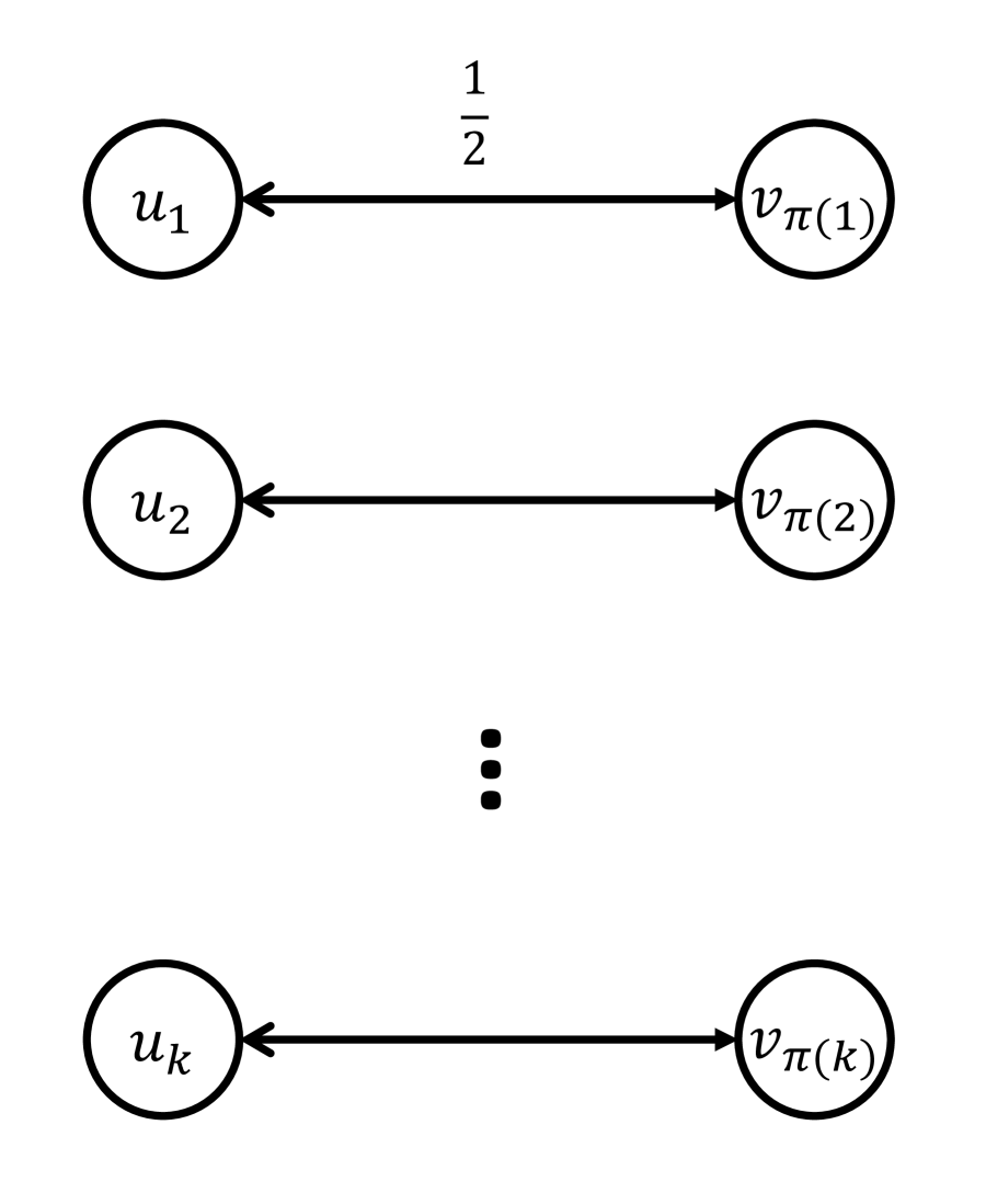
Figure 2: $(v=\pi(u))$

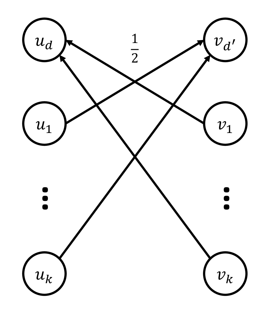
Figure 3: $(u=d\vee v=d^{\prime})$

Lemma 20.

Any unary function $f:D^{\prime}\rightarrow\mathbb{R}$ is $k$-submodular representable.

Proof.

By subtracting the minimum value of $f$, we can assume that $f$ is nonnegative. Let $d_{1}=\arg\min_{d\in D}f(x)$. Then, we construct a $(\{v\},k)$-network as follows (Figure 3):

• $c(s,v_{d_{1}})=f(0)$,

• $c(v_{d_{1}},t)=f(d_{1})$,

• $c(v_{d},t)=f(d)-f(0)$ for any $d\neq d_{1}$.

Note that, for $d\neq d_{1}$, $f(d)-f(0)\geq 0$ holds because it holds that $2f(0)\leq f(d_{1})+f(d)\leq 2f(d)$.

If $\phi(v)=0$, the capacity of the corresponding cut is $c(S_{\phi})=c(s,v_{d_{1}})=f(0)$. If $\phi(v)=d_{1}$, the capacity of the corresponding cut is $c(S_{\phi})=c(v_{d_{1}},t)=f(d_{1})$. If $\phi(v)=d$ for $d\neq d_{1}$, the capacity of the corresponding cut is $c(S_{\phi})=c(s,v_{d_{1}})+c(v_{d},t)=f(d)$. Thus the network actually represents $f$.

Let $D^{\prime}\subseteq D$ be a set of size at least $2$ and let $S=\{s\}\cup\{v_{d}\mid d\in D^{\prime}\}$ be a cut. When $D^{\prime}$ does not contain $d_{1}$, let $d_{2},d_{3}$ be distinct elements contained in $D^{\prime}$. Then, $c(S)$ is at least $c(s,v_{d_{1}})+c(v_{d_{2}},t)+c(v_{d_{3}},t)=f(d_{2})+f(d_{3})-f(0)$. Since $f$ is $k$-submodular, $f(d_{2})+f(d_{3})\geq 2f(0)$. Therefore, $c(S)\geq f(0)=c(\nu(S))$ holds. When $D^{\prime}$ contains $d_{1}$, let $d_{2}$ be another element contained in $D^{\prime}$. Then, $c(S)$ is at least $c(v_{d_{1}},t)+c(v_{d_{2}},t)=f(d_{1})+f(d_{2})-f(0)\geq f(0)$. Therefore, $c(S)\geq c(\nu(S))$ holds. Thus the network is actually $k$-submodular. ∎

Lemma 21.

For any permutation $\pi$ on $D$, the basic $k$-submodular relaxation $f$ of the soft version of a constraint $(x=\pi(y))$ is $k$-submodular representable.

Proof.

Let $u,v$ be variables. We construct a $(\{u,v\},k)$-network as follows (Figure 3):

• $c(u_{i},v_{\pi(i)})=\frac{1}{2}$ for any $i\in D$,

• $c(v_{j},u_{\pi^{-1}(j)})=\frac{1}{2}$ for any $j\in D$.

If $\phi(u)=\phi(v)=0$, the capacity of the corresponding cut is $c(S_{\phi})=0=f(\phi)$. If $\phi(u)=i\in D$ and $\phi(v)=0$, the capacity of the corresponding cut is $c(S_{\phi})=c(u_{i},v_{\pi(i)})=\frac{1}{2}=f(\phi)$. Similarly, if $\phi(u)=0$ and $\phi(v)\neq 0$, the capacity of the corresponding cut is equal to $f(\phi)$. If $\phi(u)=i\in D,\phi(v)=j\in D$ and $j=\pi(i)$, the capacity of the corresponding cut is $c(S_{\phi})=0=f(\phi)$. Otherwise, the capacity of the corresponding cut is $c(S_{\phi})=c(u_{i},v_{\pi(i)})+c(v_{j},u_{\pi^{-1}(j)})=1=f(\phi)$. Thus the network actually represents $f$.

Let $S$ be a cut and $I,J$ be two sets such that $I=\{i\in D\mid u_{i}\in S\}$ and $J=\{j\in D\mid v_{j}\in S\}$. If $|I|\leq 1$ and $|J|\leq 1$, the cut $S$ is already normalised. If $|I|=0$ or $|I|\geq 2$, and $|J|=0$ or $|J|\geq 2$, the capacity of the normalised cut is $c(\nu(S))=c(\{s\})=0$ and the capacity of the original cut is nonnegative. Therefore, $c(S)\geq c(\nu(S))$ holds. If $I=\{i\}$ and $|J|\geq 2$, the capacity of the normalised cut is $c(\nu(S))=c(\{s,u_{i}\})=c(u_{i},v_{\pi(i)})=\frac{1}{2}$. Because $\pi$ is a permutation, for at least one $j\in J$, $\pi^{-1}(j)$ is different from $i$. Therefore, the capacity of the original cut is at least $\frac{1}{2}$. Thus, it holds that $c(S)\geq c(\nu(S))$. Similarly, if $|I|\geq 2$ and $|J|=1$, it holds that $c(S)\geq c(\nu(S))$. Thus, the network is actually $k$-submodular. ∎

Lemma 22.

For any $d,d^{\prime}\in D$, the basic $k$-submodular relaxation $f$ of the soft version of a constraint $(x=d\vee y=d^{\prime})$ is $k$-submodular representable.

Proof.

Let $u,v$ be variables. We construct a $(\{u,v\},k)$-network as follows (Figure 3):

• $c(u_{i},v_{d^{\prime}})=\frac{1}{2}$ for any $i\in D\setminus\{d\}$,

• $c(v_{j},u_{d})=\frac{1}{2}$ for any $j\in D\setminus\{d^{\prime}\}$.

If $\phi(u)=\phi(v)=0$, $\phi(u)=d$, or $\phi(v)=d^{\prime}$, the capacity of the corresponding cut is $c(S_{\phi})=0=f(\phi)$. If $\phi(u)=i\in D\setminus\{d\}$ and $\phi(v)=0$, the capacity of the corresponding cut is $c(S_{\phi})=c(u_{i},v_{d}^{\prime})=\frac{1}{2}=f(\phi)$. Similarly, if $\phi(u)=0$ and $\phi(v)\in D\setminus\{d^{\prime}\}$, the capacity of the corresponding cut is equal to $f(\phi)$. If $\phi(u)=i\in D\setminus\{d\},\phi(v)=j\in D\setminus\{d^{\prime}\}$, the capacity of the corresponding cut is $c(S_{\phi})=c(u_{i},v_{d^{\prime}})+c(v_{j},u_{d})=1=f(\phi)$. Thus the network actually represents $f$.

Let $S$ be a cut and $I,J$ be two sets such that $I=\{i\in D\mid u_{i}\in S\}$ and $J=\{j\in D\mid v_{j}\in S\}$. If $|I|\leq 1$ and $|J|\leq 1$, the cut $S$ is already normalised. If $|I|=0$ or $|I|\geq 2$, and $|J|=0$ or $|J|\geq 2$, the capacity of the normalised cut is $c(\nu(S))=c(\{s\})=0$ and the capacity of the original cut is nonnegative. Therefore, $c(S)\geq c(\nu(S))$ holds. If $I=\{d\}$ and $|J|\geq 2$, both of the normalised cut and the original cut have the capacity zero. If $I=\{i\}$ for $i\neq d$ and $|J|\geq 2$, since $J$ contains at least one element $j$ which is different from $d^{\prime}$, the capacity of the original cut is at least $c(v_{j},u_{d})=\frac{1}{2}$. On the other hand, the capacity of the normalised cut is $c(\nu(S))=c(u_{i},v_{d}^{\prime})=\frac{1}{2}$. Therefore, it holds that $c(S)\geq c(\nu(S))$. Similarly, if $|I|\geq 2$ and $|J|=1$, it holds that $c(S)\geq c(\nu(S))$. Thus, the network is actually $k$-submodular. ∎

Finally, we prove Theorem 3.

Proof of Theorem 3.

By using Lemmas 20–22, we can construct a $k$-submodular $(X,k)$-network $(G,c)$ that represents $f$ in $O(|G|)$ time. Since we create $O(k)$ edges per each summand function $f_{i}$, the size of the network is $O(km)$. Because the capacity of the minimum cut of the network is equal to $\min f$ and each capacity is a multiple of $\frac{1}{2}$, we can compute the maximum flow of the network in $O((\min f)km)$ time. Then, by using Lemma 19, we can compute an extreme minimum cut in $O(km)$ time. Finally, by using Lemma 17, we can obtain an extreme minimum solution. The total running time is $O((\min f)km)$. ∎

7 Conclusions and open problems

We have shown that half-integrality and LP-branching can be powerful tools for FPT-algorithms, beyond just Vertex Cover and Multiway Cut. We have outlined how to use CSP tools to find and study such relaxations. As an application, we have given new half-integral relaxations for Unique Label Cover and Group Feedback Vertex Set, in both cases improving the running time asymptotically (to single-exponential for fixed label set, resp. to unconditionally single-exponential). Several directions of further study suggest themselves. Is there a way to decide the existence of discrete relaxations in general? Can directed problems, e.g., Directed Feedback Vertex Set be handled in a similar manner? Finally, can the basic tool of LP-branching be complemented with more sophisticated algorithmic approaches (e.g., FPT-time separation oracles, or tools from semi-definite programming)?

In other directions, we note that several of the covered problems have polynomial kernels for specific cases, e.g., Group Feedback Vertex Set with bounded-size group [39] and Feedback Vertex Set [53]; it is an interesting question how far this can be generalised.

We also note that oracle minimisation of $k$-submodular functions is an open question; we also welcome more investigation into $k$-submodular functions in general (including, e.g., any possible connections to path-packing systems as in [13, 14, 44, 45], and algebraic algorithms generalising those for matching; see also [54]).

As for linear-time complexity, we have shown that edge-deletion Unique Label Cover can be solved in linear-time. It is known that Multiway Cut, a special case of Unique Label Cover, can be solved in linear-time even for the node-deletion version [31]. It is an interesting question whether node-deletion Unique Label Cover can also be solved in linear-time. In order to obtain linear-time FPT algorithms, we have shown that we can minimize a sum of basic binary $k$-submodular functions via network flow. We left whether it is possible to minimize a sum of any binary $k$-submodular functions in a similar way or not as an open problem.

Appendix A On the crisp solution structure supported by the algorithms

Now, we discuss the crisp solution structure supported by bisubmodular and $k$-submodular functions (in particular, we prove Lemma 4).

To illustrate the topic, let us focus on the (well-understood) case of submodular functions. It is known that for a submodular function $f:2^{V}\rightarrow\mathbb{R}$, one can not only minimise $f(S)$ efficiently in an unconstrained setting, but also subject to a ring family. Recall that a ring family is a set family ${\cal{F}}\subseteq 2^{V}$ which is closed under union and intersection, i.e., if $A,B\in{\cal{F}}$ then $A\cup B,A\cap B\in\cal{F}$. The constrained optimisation problem is then $\min_{S\in{\cal{F}}}f(S),$ which can be solved in polynomial time even if $f$ is only given via oracle access (see Schrijver [50]).

Now observe that the conditions on a ring family are actually polymorphisms of the relation $R(S)=(S\in\cal{F})$. Indeed, it is known that a relation $R\subseteq 2^{V}$ is closed under union and intersection if and only if $R$ can be modelled as the set of solutions to a formula using constraints $(x\rightarrow y)$, $(x=0)$, and $(x=1)$ (e.g., the set of closed vertex sets in a digraph). Furthermore, if $f$ is a submodular function, then the set of minimising assignments ${\cal{A}}=\{A\subseteq V:f(A)=\min_{S}f(S)\}$ is itself closed under union and intersection (by applying the submodularity condition $f(A)+f(B)\geq f(A\cap B)+f(A\cup B)$ to two minimising assignments $A,B\in{\cal{A}}$). Thus, if we want to implement some crisp solution structure on the search space $2^{V}$ by only using the power of submodular functions, then this restriction must take the shape of a ring family, and if it does, then it is sufficient to implement the crisp constraints $(x\rightarrow y),(x=0)$, and $(x=1)$, which can be done by using their soft versions at very high cost; these soft versions are submodular, which closes the loop.

Expressed more succinctly, if one wants to perform constrained minimisation of a submodular function without using any algorithm more powerful than basic (unconstrained) submodular minimisation, then the power one has at hand is exactly that of crisp implications and assignments. We will investigate the same for functions with bisubmodular or $k$-submodular relaxations. Let us finally remark that this is not a restriction on submodular functions themselves; submodular functions in general are far more expressive than digraph cut functions (this has been proven formally in [55]).

A.1 Bisubmodular relaxations

We now consider the bisubmodular case of the above, i.e., relaxations of functions $f_{i}:2^{V}\rightarrow\mathbb{R}$ into bisubmodular functions $f_{i}^{\prime}:\{0,{\nicefrac{{1}}{{2}}},1\}^{V}\rightarrow\mathbb{R}$. We consider the structure of the minimising set ${\cal{A}}$ when restricted to integral assignments (i.e., those half-integral minimisers of $f^{\prime}$ which happen to also be integral; note that this may well be an empty set). We find that Bisubmodular Cost 2-SAT exactly captures its structure.

Lemma 23.

Let $f:\{0,{\nicefrac{{1}}{{2}}},1\}^{V}\rightarrow\mathbb{R}$ be a bisubmodular function, and ${\cal{A}}\subseteq\{0,{\nicefrac{{1}}{{2}}},1\}^{V}$ be its set of minimising assignments. Then the integral global minimisers ${\cal{A}}\cap\{0,1\}^{V}$ of $f$ can be modelled as the set of solutions to a (crisp) 2-CNF formula $F$ on $V$.

Proof.

Let ${\cal{A}}_{01}={\cal{A}}\cap\{0,1\}^{V}$. We will show that ${\cal{A}}_{01}$ can be described by a 2-CNF formula. As discussed above for the submodular case, ${\cal{A}}$ as a whole must be closed under the operations $\sqcap$ and $\sqcup$, i.e., $\sqcup$ and $\sqcap$ are polymorphisms of ${\cal{A}}$. Define $h(A,B,C)=(((A\sqcap B)\sqcup(A\sqcap C))\sqcup(B\sqcap C))$; then $h$ is a ternary polymorphism of ${\cal{A}}$, and it can be verified that $h$ is a majority operation. Thus ${\cal{A}}$ is fully described by the binary constraints that it implies (see preliminaries). In turn, each binary constraint $R(x,y)$ can of course be described by enumerating the forbidden values of the pair $(x,y)$. Thus, for every point in $\phi\in\{0,1\}^{n}$ which is not a point of ${\cal{A}}_{01}$, there is a binary constraint $R(x,y)$ which rejects it. All such binary constraints on $\{0,1\}$ can be described via 2-clauses. ∎

A.2 $k$-Submodular relaxations

For $k>2$, the situation is more complicated than above. The setup is the same: if ${\cal{A}}\subseteq\{0,\ldots,k\}^{V}$ is the set of minimising assignments to a $k$-submodular function $f$, then we look at the structure of the subset ${\cal{A}}_{\mathrm{int}}={\cal{A}}\cap\{1,\ldots,k\}^{V}$ of those assignments which are also integral. As before, the structure can be defined by a formula over binary (crisp) constraints, however, the set of binary constraints we can use is limited. As stated in Lemma 4, it turns out that the binary constraints of Lemma 3 is exactly the right list.

Proof of Lemma 4..

To begin with, we observe as in the proof of Lemma 23 that binary (and unary) constraints must suffice to describe the structure. In fact, the same construction of a majority polymorphism $h(A,B,C)$ from $\sqcap$ and $\sqcup$ applies directly for $k>2$, hence ${\cal{A}}$, and by implication ${\cal{A}}_{\mathrm{int}}$, is fully characterised by its 2-variable projections. The remaining task is thus to characterise those crisp binary constraints on domain $\{1,\ldots,k\}$ whose soft versions have bisubmodular relaxations. By Lemma 3, we can support arbitrary unary constraints, thus we focus on the properly binary constraints.

For the rest of the proof, we let $R\subseteq\{0,\ldots,k\}^{2}$ be a binary relation closed under $\sqcup$ and $\sqcap$. We will characterise the possible sets $R\cap\{1,\ldots,k\}^{2}$ of integral pairs satisfying $R$. Let $S_{1}=\{a\in\{1,\ldots,k\}:(a,b)\in R\text{ for some }b\}$ and $S_{2}=\{b\in\{1,\ldots,k\}:(a,b)\in R\text{ for some }a\}$ be the integral values that occur in positions $1$ and $2$ of $R$, respectively; they can be assumed to be non-empty, as otherwise $R$ is simply a conjunction of an assignment and a unary constraint.

We begin by a useful property.

Claim 10.

If $(a,0)\in R$ for some $a\in S_{1}$, then for every $b\in S_{2}$ we have $(a,b)\in R$. Thus in particular, for every $a\in S_{1}$ there is some $b\in S_{2}$ such that $(a,b)\in R$.

Proof.

If $(0,b)\in R$, then we have $(a,b)\in R$ by $(a,0)\sqcup(0,b)=(a,b)$.

On the other hand, if $(a^{\prime},b)\in R$ for some $a^{\prime}\in S_{1}$ with $a^{\prime}\neq a$, then $(0,b)\in R$ by $(a^{\prime},b)\sqcup(a,0)=(0,b)$, and we are back in the first case. ∎

We eliminate some quick corner cases. Recall that we are focusing on expressing ${\cal{A}}_{\mathrm{int}}$ via binary relations, rather than all of ${\cal{A}}$; hence if the intersection of $R$ with $\{1,\ldots,k\}^{2}$ is simple, we may ignore complications involving the value $0$. In particular, consider the case that $|S_{1}|=1$, say $S_{1}=\{a\}$. By the above, $(a,b)\in R$ for every $b\in S_{2}$, implying that the effect of $R(x,y)$ on ${\cal{A}}_{\mathrm{int}}$ is simply the conjunction of $(x=a)$ and $(y\in S_{2})$. We claim similarly if $|S_{2}|=1$. Thus in the sequel, we have $|S_{1}|,|S_{2}|>1$.

We give the next useful observation.

Claim 11.

For any $a\in S_{1}$, either there is exactly one value $b\in S_{2}$ such that $(a,b)\in R$, or $(a,b)\in R$ for every $b\in S_{2}$. Symmetrically, for any $b\in S_{2}$, either there is exactly one value $a\in S_{1}$ such that $(a,b)\in R$, or $(a,b)\in R$ for every $b\in S_{1}$.

Proof.

We prove the claim for some $a\in S_{1}$; the other half is entirely symmetric. Recall that $(a,b)\in R$ for at least one $b\in S_{2}$, by previous claims. Thus let $(a,d),(a,d^{\prime})\in S$ for $d,d^{\prime}\in S_{2}$, $d\neq d^{\prime}$; this produces $(a,0)\in R$ via the polymorphism $\sqcup$, and by the previous claim $(a,b)\in R$ for every $b\in S_{2}$, as claimed. ∎

We call a value $a\in S_{1}$ (resp. $b\in S_{2}$) global if the second case occurs, i.e., if $(a,d)\in R$ for every $d\in S_{2}$ (resp. $(d,b)\in R$ for every $d\in S_{1}$). We may assume that each of $S_{1}$ and $S_{2}$ contains at most one global value: if $S_{1}$ contains two global values $a,a^{\prime}$, then every value in $S_{2}$ must be global, and since $|S_{2}|>1$ we get that every value in $S_{1}$ is global, and the effect of $R$ on ${\cal{A}}_{\mathrm{int}}$ can be described via unary constraints.

Furthermore, if $a\in S_{1}$ and $b\in S_{2}$ are global values, then for any $a^{\prime}\in S_{1}$, $a^{\prime}\neq a$, we have that $(a^{\prime},b)\in R$ is the unique occurrence of $a^{\prime}$ in $R$; hence the effect of $R(x,y)$ on ${\cal{A}}_{\mathrm{int}}$ can be given as $(x=a\lor y=b)$ in conjunction with unary constraints. Note that this is case 3 of Lemma 3.

Second, assume that $S_{2}$ contains no global values, but $a\in S_{1}$ is global. But there is one further $a^{\prime}\in S_{1}$, with $(a^{\prime},b)\in R$ for some $b\in S_{2}$ by Claim 10; hence $b$ is global and we are back at a previous case.

Finally, if there are no global values, then the values of $S_{1}$ and $S_{2}$ must be matched to each other with exactly one possible value each. We may thus describe $R$ as a bijection $(x=\pi(y))$ in conjunction with a unary constraint, i.e., case 2 of Lemma 3. This finishes the proof. ∎

Note that this is not a complete characterisation of the full set ${\cal{A}}$ of minimisers, since we skipped some “corner cases” that become uninteresting when intersected with $\{1,\ldots,k\}^{V}$. Also note, as in the discussion for submodular functions, that this does not imply that Lemma 3 can produce all functions with $k$-submodular relaxations, as valued constraints taking several values (beyond $0$ and $1$) are not covered, and these may well be the most interesting cases (cf. matroids for the submodular case).

Appendix B Basic $k$-submodular functions: Case analysis

Finally, we go through the case analysis required to show that all the relaxations listed in the proof sketch of Lemma 3 are actually $k$-submodular.

Full proof of Lemma 3..

Case 1. Let $f$ be a unary function of $\{1,\ldots,k\}$, and $f^{\prime}$ the relaxation to $\{0,\ldots,k\}$ as in the proof sketch. Consider two domain values $x$ and $y$. If $x$ and $y$ are integral and distinct, then $x\sqcap y=x\sqcup y=0$, and the inequality holds; otherwise, the outputs $x\sqcap y$ and $x\sqcup y$ are a reordering of the inputs.

Case 2. For the bijection case, let $f$ be the relaxation, and consider two evaluations $f(x_{1},y_{1})$ and $f(x_{2},y_{2})$. We refer to $(x_{1},y_{1})$ and $(x_{2},y_{2})$ as the input, and the tuples of the resulting right-hand-side (after application of $\sqcap$ and $\sqcup$) as the output. We split the proof by the number of variables $x_{1},y_{1},x_{2},y_{2}$ that take the value zero. If none of them takes the value zero, then either the output equals the input, or the output is all-zero, or the output has one all-zero column and the input costs at least $1$; all these satisfy the $k$-submodularity inequality. If one input, say $(x_{1},y_{1})$, equals $(0,0)$, then the output equals the input.

If exactly one value is zero, assume w.l.o.g. that $x_{1}=d$ and $x_{2}=0$; the same two values occur in the output (in the first “column”), and we note that the other two output values (the second “column”) equal each other. Thus either the output equals the input, or the output has an all-zero column and cost $\nicefrac{{1}}{{2}}$, while the input costs at least as much.

If $x_{1}=x_{2}=0$ but $y_{1},y_{2}\neq 0$ (or similarly with $x$ and $y$ swapped), then either the output equals the input, or the output has cost zero. Finally, with two zero-values in different columns and tuples, the input costs ${\nicefrac{{1}}{{2}}}+{\nicefrac{{1}}{{2}}}$ and the output contains one tuple $(0,0)$ at cost zero. This finishes the case.

Case 3. Let $f_{a,b}$ be the function defined in the proof sketch; we show that it is $k$-submodular.

Refer to $a$ in the first coordinate, or $b$ in the second coordinate, as a safe coordinate; note that $f_{a,b}$ can be viewed as taking cost $0$ if at least one coordinate is safe, and otherwise $\nicefrac{{1}}{{2}}$ times the number of non-safe integral coordinates. We split into cases. First, assume that one column of the output contains two integral non-safe values. Then this column must be constant in input and output. If the other output column contains two zeros, then the output costs $1$ and the input costs either at least $1+0$ or ${\nicefrac{{1}}{{2}}}+{\nicefrac{{1}}{{2}}}$. With one zero, the output is a reordering of the input, and nothing is changed. With no zeros, input and output are constant and identical.

Second, assume that both output columns contain one non-safe integral value each. Then the output is $(0,0)$ and $(d,d^{\prime})$, where $d$ and $d^{\prime}$ are non-safe, but then the output columns are just reorderings of the input columns, so the input costs either ${\nicefrac{{1}}{{2}}}+{\nicefrac{{1}}{{2}}}$ or $1+0$.

In the last cases, the total number of non-safe integral values in the output is either $0$, at output cost zero, or $1$. In the last case, the maximum total output cost is $\nicefrac{{1}}{{2}}$, in which case the non-safe column of the output is $0,d$ for some $d$, the parallel column is $0,0$, and the input contains either a tuple $(d,0)$ or $(0,d^{\prime})$ for unsafe integral values $d,d^{\prime}$.

Case 4. We show $k$-submodularity. Consider the total cost of the input. If the input has total cost zero, then the output is either all-zero or identical to the input. If the input has a tuple of cost zero, it must be constant, say $(x,\ldots,x)$. If $x=0$, then the output equals the input; otherwise, the output uses only values $0$ and $x$. The $\sqcap$-tuple contains $x$ if and only if $x$ occurs in the other tuple; the $\sqcup$-tuple contains $0$ if and only if some $d^{\prime}\notin\{0,d\}$ occurs in the other tuple. Each event “costs” at most $\nicefrac{{1}}{{2}}$, and if both events occur, the input costs $1$.

If the input cost is ${\nicefrac{{1}}{{2}}}+{\nicefrac{{1}}{{2}}}$, then there are similarly two essential cases (the non-zero entries are identical or different), both of which have an output of total cost at most $1$. Otherwise, the input costs at least $1+{\nicefrac{{1}}{{2}}}$, and the output can only cost $1+1$ if there are two distinct constant non-zero columns in the input (in which case the input costs $1+1$). ∎

References

- [1] 53rd Annual IEEE Symposium on Foundations of Computer Science, FOCS 2012, New Brunswick, NJ, USA, October 20-23, 2012. IEEE Computer Society, 2012.
- [2] H. L. Bodlaender. A linear-time algorithm for finding tree-decompositions of small treewidth. SIAM Journal on Computing, 25(6):1305–1317, 1996.
- [3] A. Bouchet. Coverings and delta-coverings. In E. Balas and J. Clausen, editors, IPCO, volume 920 of Lecture Notes in Computer Science, pages 228–243. Springer, 1995.
- [4] A. Bouchet. Multimatroids I. Coverings by independent sets. SIAM J. Discrete Math., 10(4):626–646, 1997.
- [5] A. Bouchet. Multimatroids II. Orthogonality, minors and connectivity. Electr. J. Comb., 5, 1998.
- [6] A. Bouchet. Multimatroids IV. Chain-group representations. Linear Algebra and its Applications, 277(1-3):271–289, 1998.
- [7] A. Bouchet. Multimatroids III. Tightness and fundamental graphs. Eur. J. Comb., 22(5):657–677, 2001.
- [8] A. Bouchet and W. H. Cunningham. Delta-matroids, jump systems, and bisubmodular polyhedra. SIAM J. Discrete Math., 8(1):17–32, 1995.
- [9] J. Chen, B. Chor, M. Fellows, X. Huang, D. W. Juedes, I. A. Kanj, and G. Xia. Tight lower bounds for certain parameterized NP-hard problems. Inf. Comput., 201(2):216–231, 2005.
- [10] J. Chen, X. Huang, I. A. Kanj, and G. Xia. Strong computational lower bounds via parameterized complexity. J. Comput. Syst. Sci., 72(8):1346–1367, 2006.
- [11] R. H. Chitnis, M. Cygan, M. Hajiaghayi, M. Pilipczuk, and M. Pilipczuk. Designing FPT algorithms for cut problems using randomized contractions. In FOCS [1], pages 460–469.
- [12] F. A. Chudak, M. X. Goemans, D. S. Hochbaum, and D. P. Williamson. A primal-dual interpretation of two 2-approximation algorithms for the feedback vertex set problem in undirected graphs. Oper. Res. Lett., 22(4-5):111–118, 1998.
- [13] M. Chudnovsky, W. H. Cunningham, and J. Geelen. An algorithm for packing non-zero A-paths in group-labelled graphs. Combinatorica, 28(2):145–161, 2008.
- [14] M. Chudnovsky, J. Geelen, B. Gerards, L. A. Goddyn, M. Lohman, and P. D. Seymour. Packing non-zero A-paths in group-labelled graphs. Combinatorica, 26(5):521–532, 2006.
- [15] M. C. Cooper, D. A. Cohen, and P. Jeavons. Characterising tractable constraints. Artif. Intell., 65(2):347–361, 1994.
- [16] M. Cygan, J. Nederlof, M. Pilipczuk, M. Pilipczuk, J. M. M. van Rooij, and J. O. Wojtaszczyk. Solving connectivity problems parameterized by treewidth in single exponential time. In R. Ostrovsky, editor, FOCS, pages 150–159. IEEE, 2011.
- [17] M. Cygan, M. Pilipczuk, and M. Pilipczuk. On group feedback vertex set parameterized by the size of the cutset. In M. C. Golumbic, M. Stern, A. Levy, and G. Morgenstern, editors, WG, volume 7551 of Lecture Notes in Computer Science, pages 194–205. Springer, 2012.
- [18] M. Cygan, M. Pilipczuk, M. Pilipczuk, and J. O. Wojtaszczyk. On multiway cut parameterized above lower bounds. TOCT, 5(1):3, 2013.
- [19] M. Cygan, M. Pilipczuk, M. Pilipczuk, and J. O. Wojtaszczyk. Subset feedback vertex set is fixed-parameter tractable. SIAM J. Discrete Math., 27(1):290–309, 2013.
- [20] L. Fleischer, K. Jain, and D. P. Williamson. Iterative rounding 2-approximation algorithms for minimum-cost vertex connectivity problems. J. Comput. Syst. Sci., 72(5):838–867, 2006.
- [21] S. Fujishige and S. Iwata. Bisubmodular function minimization. SIAM J. Discrete Math., 19(4):1065–1073, 2005.
- [22] N. Garg, V. V. Vazirani, and M. Yannakakis. Primal-dual approximation algorithms for integral flow and multicut in trees. Algorithmica, 18(1):3–20, 1997.
- [23] N. Garg, V. V. Vazirani, and M. Yannakakis. Multiway cuts in node weighted graphs. J. Algorithms, 50(1):49–61, 2004.
- [24] S. Guillemot. FPT algorithms for path-transversal and cycle-transversal problems. Discrete Optimization, 8(1):61–71, 2011.
- [25] D. S. Hochbaum. Solving integer programs over monotone inequalities in three variables: A framework for half integrality and good approximations. European Journal of Operational Research, 140(2):291–321, 2002.
- [26] A. Huber and V. Kolmogorov. Towards minimizing k-submodular functions. In A. R. Mahjoub, V. Markakis, I. Milis, and V. T. Paschos, editors, ISCO, volume 7422 of Lecture Notes in Computer Science, pages 451–462. Springer, 2012.
- [27] K. ichi Kawarabayashi and P. Wollan. Non-zero disjoint cycles in highly connected group labelled graphs. J. Comb. Theory, Ser. B, 96(2):296–301, 2006.
- [28] R. Impagliazzo, R. Paturi, and F. Zane. Which problems have strongly exponential complexity? J. Comput. Syst. Sci., 63(4):512–530, 2001.
- [29] S. Iwata, L. Fleischer, and S. Fujishige. A combinatorial strongly polynomial algorithm for minimizing submodular functions. J. ACM, 48(4):761–777, 2001.
- [30] S. Iwata and K. Nagano. Submodular function minimization under covering constraints. In FOCS, pages 671–680. IEEE Computer Society, 2009.
- [31] Y. Iwata, K. Oka, and Y. Yoshida. Linear-time FPT algorithms via network flow. In SODA, pages 1749–1761, 2014.
- [32] K. Jain. A factor 2 approximation algorithm for the generalized Steiner network problem. Combinatorica, 21(1):39–60, 2001.
- [33] P. Jeavons, D. A. Cohen, and M. C. Cooper. Constraints, consistency and closure. Artif. Intell., 101(1-2):251–265, 1998.
- [34] P. Jonsson, F. Kuivinen, and J. Thapper. Min CSP on four elements: Moving beyond submodularity. In J. H.-M. Lee, editor, CP, volume 6876 of Lecture Notes in Computer Science, pages 438–453. Springer, 2011.
- [35] K. Kawarabayashi and B. A. Reed. Computing crossing number in linear time. In STOC’07: Proceedings of the 39th Annual ACM Symposium on Theory of Computing, pages 382–390, 2007.
- [36] S. Khot. On the power of unique 2-prover 1-round games. In J. H. Reif, editor, STOC, pages 767–775. ACM, 2002.
- [37] V. Kolmogorov. Generalized roof duality and bisubmodular functions. Discrete Applied Mathematics, 160(4-5):416–426, 2012.
- [38] V. Kolmogorov. The power of linear programming for valued CSPs: a constructive characterization. CoRR, abs/1207.7213, 2012.
- [39] S. Kratsch and M. Wahlström. Representative sets and irrelevant vertices: New tools for kernelization. In FOCS, pages 450–459, 2012.
- [40] D. Lokshtanov, N. S. Narayanaswamy, V. Raman, M. S. Ramanujan, and S. Saurabh. Faster parameterized algorithms using linear programming. CoRR, abs/1203.0833, 2012.
- [41] N. S. Narayanaswamy, V. Raman, M. S. Ramanujan, and S. Saurabh. LP can be a cure for parameterized problems. In C. Dürr and T. Wilke, editors, STACS, volume 14 of LIPIcs, pages 338–349. Schloss Dagstuhl - Leibniz-Zentrum fuer Informatik, 2012.
- [42] G. Nemhauser and L. Trotter. Vertex packing: structural properties and algorithms. Mathematical Programming, 8:232–248, 1975.
- [43] J. Oxley. Matroid Theory. Oxford Graduate Texts in Mathematics. Oxford University Press, 2006.
- [44] G. Pap. Packing non-returning -paths. Combinatorica, 27(2):247–251, 2007.
- [45] G. Pap. Packing non-returning A-paths algorithmically. Discrete Mathematics, 308(8):1472–1488, 2008.
- [46] J.-C. Picard and M. Queyranne. On the structure of all minimum cuts in a network and applications. In V. Rayward-Smith, editor, Combinatorial Optimization II, volume 13 of Mathematical Programming Studies, pages 8–16. Springer Berlin Heidelberg, 1980.
- [47] P. Raghavendra. Optimal algorithms and inapproximability results for every CSP? In C. Dwork, editor, STOC, pages 245–254. ACM, 2008.
- [48] M. S. Ramanujan and S. Saurabh. Linear time parameterized algorithms via skew-symmetric multicuts. In SODA, pages 1739–1748, 2014.
- [49] A. Schrijver. A combinatorial algorithm minimizing submodular functions in strongly polynomial time. J. Comb. Theory, Ser. B, 80(2):346–355, 2000.
- [50] A. Schrijver. Combinatorial Optimization: Polyhedra and Efficiency. Algorithms and combinatorics. Springer, 2003.
- [51] J. Thapper and S. Zivny. The power of linear programming for valued CSPs. In FOCS [1], pages 669–678.
- [52] J. Thapper and S. Zivny. The complexity of finite-valued CSPs. In D. Boneh, T. Roughgarden, and J. Feigenbaum, editors, STOC, pages 695–704. ACM, 2013.
- [53] S. Thomassé. A 4k kernel for feedback vertex set. ACM Transactions on Algorithms, 6(2), 2010.
- [54] Y. Yamaguchi. Packing a-paths in group-labelled graphs via linear matroid parity. In SODA, pages 562–569, 2014.
- [55] S. Živný, D. A. Cohen, and P. G. Jeavons. The expressive power of binary submodular functions. Discrete Applied Mathematics, 157(15):3347–3358, 2009.