Coupled plasmon - phonon excitations in extrinsic monolayer graphene

Abstract

The existence of an acoustic plasmon in extrinsic (doped or gated) monolayer graphene was found recently in an ab initio calculation with the frozen lattice [M. Pisarra et al., arXiv:1306.6273, 2013]. By the fully dynamic density-functional perturbation theory approach, we demonstrate a strong coupling of the acoustic plasmonic mode to lattice vibrations. Thereby, the acoustic plasmon in graphene does not exist as an isolated excitation, but it is rather bound into a combined plasmon-phonon mode. We show that the coupling provides a mechanism for the bidirectional energy exchange between the electronic and the ionic subsystems with fundamentally, as well as practically, important implications for the lattice cooling and heating by electrons in graphene.

Known for its extraordinary properties and vast potential applications Castro Neto et al. (2009), graphene – a two-dimensional crystal comprised of a honeycomb lattice of carbon atoms – continues to receive much attention as it reveals new remarkable features Park et al. (2009); Kogan and Nazarov (2012); Kogan (2013); Nazarov et al. (2013); Kang et al. (2013); Pisarra et al. (2013). For one of the recent findings, an acoustic plasmon (APl) (plasmon with linear wave-vector dispersion) has been predicted theoretically in an extrinsic free-standing monolayer graphene Pisarra et al. (2013). This finding is extraordinary considering that APl generation conventionally involves a surface state immersed in the bulk of a metal Pitarke et al. (2004).

Exhibiting linear wave-vector dispersion, acoustic APl persists down to low frequencies, where it can be expected to interact with phonon oscillations. The possibility of coupling these two types of elementary excitations motivates questions of fundamental physics as well as of potential applications. In this Letter we show that the APl - phonon coupling indeed occurs in the electron-doped graphene and it provides a mechanism for the bidirectional energy exchange between the electronic and ionic subsystems. The conventional treatment of lattice vibrations by frequency-independent density-functional perturbation theory (DFPT) Giannozzi and Baroni (2005) is inadequate for capturing the essentially dynamic nature of the coupled plasmon-phonon modes, and we therefore implement a fully dynamic approach treating the electron-hole, plasmon, and phonon elementary excitations on the equal footing Bostwick et al. (2007).

Our ab initio calculations for monolayer graphene employ the full-potential linear augmented plane-wave (FP-LAPW) code Elk Elk . The super-cell geometry is utilized with a separation of the layers in the $z$ direction of 40 bohr, which effectively ensures the non-interaction between the layers. The local-density approximation to the exchange-correlation potential Dirac (1930); Perdew and Wang (1992) is used.

Acoustic-plasmon and phonons in graphene.– We start by reproducing the APl and phonon spectra of graphene without the coupling of the two excitations. In Fig. 1, left panel, the energy-loss function of graphene is plotted for a number of equidistant values of the wave-vector. The calculation with the carbon atoms fixed at their equilibrium positions has been used. The APl can be easily recognized by the linear dispersion of the peak with the wave-vector, which is in agreement with the recent findings in extrinsic graphene obtained with the use of the pseudopotential method Pisarra et al. (2013). In Fig. 1, right panel, we plot the phonon dispersion spectra in graphene together with the APl dispersion derived from the energy-loss function. Acoustic plasmonic and optical phononic (OPh) dispersion curves intersect, which fact suggests their interaction and constitutes the main motivation of the subsequent study of the coupled modes.

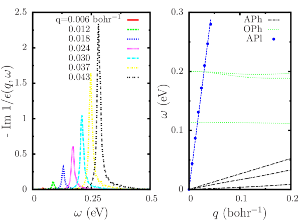
Figure 1: (color online) Left: Energy-loss function of the monolayer graphene doped with $\frac{1}{16}$ electrons per unit cell ($1.19\times 10^{14}$ cm^-2). Plasmon peaks with linear (acoustic) dispersion are dominant in the low-frequency range of the spectra. The direction of the wave-vector $q$ is along the primitive reciprocal lattice vector. Right: Phonons (acoustic, black dash-dotted lines, optical, green dotted lines, respectively) and acoustic plasmon (blue symbols) dispersion. Blue dashed line is the linear best fit to the acoustic plasmon dispersion.

Coupled plasmon-phonon modes.– We treat the problem of coupled plasmon-phonon oscillations within the dynamic (frequency-dependent) linear-response theory: Self-consistently, ions are driven by an externally applied AC electric field and by the Coulomb field of moving electrons, and in turn, electrons move under the action of the external field and the field of moving ions. We consider an infinite two-dimensional (2D) crystal lying in the $xy$ plane. The 2D lattice vectors are denoted by $\mathbf{R}$ while the position of the $\alpha$-th atom within the unit cell is $\mathbf{b}_{\alpha}$. A weak external potential of the form

$$\delta\phi^{\textit{ext}}(\mathbf{r},t)=\delta\phi^{\textit{ext}}(\mathbf{q},z,\omega)e^{i(\mathbf{q}\cdot\mathbf{r}-\omega t)}$$ (1)

is applied to the system, where $\mathbf{r}$ is the 3D position coordinate vector and $\mathbf{q}$ is the 2D wave-vector. We seek the response including the ionic oscillations around their equilibrium positions with the displacements given by

$$\mathbf{u}_{\alpha\mathbf{R}}(t)=\mathbf{u}_{\alpha\mathbf{R}}(\omega)e^{-i\omega t}=\mathbf{e}_{\alpha}e^{i(\mathbf{q}\cdot\mathbf{R}-\omega t)}$$ (2)

with 3D vectors $\mathbf{e}_{\alpha}$. The total Coulomb potential in the system is

$$\phi(\mathbf{r},t)=\phi_{0}(\mathbf{r})+\delta\phi(\mathbf{r})e^{-i\omega t},$$ (3)

where $\phi_{0}$ is the ground-state Coulomb potential and $\delta\phi$ is its first-order perturbation. The force experienced by the $\alpha$-th ion in the $\mathbf{R}$-th unit cell is

$$\mathbf{F}_{\alpha\mathbf{R}}(t)=-\left.Z_{\alpha}\nabla\phi^{\textit{eff}}_{\alpha\mathbf{R}}(\mathbf{r},t)\right|_{\mathbf{r}=\mathbf{b}_{\alpha}+\mathbf{u}_{\alpha\mathbf{R}}(t)+\mathbf{R}},$$ (4)

where $Z_{\alpha}$ is the charge of the $\alpha$-th ion within the unit cell and $\phi^{\textit{eff}}_{\alpha\mathbf{R}}$ is the total Coulomb potential minus the self-interaction of the $(\alpha\mathbf{R})$-th ion

$$\phi^{\textit{eff}}_{\alpha\mathbf{R}}(\mathbf{r},t)=\phi(\mathbf{r},t)-\frac{Z_{\alpha}}{|\mathbf{r}-\mathbf{b}_{\alpha}-\mathbf{u}_{\alpha\mathbf{R}}(t)-\mathbf{R}|}.$$ (5)

Expansion of Eq. (5) to the first order in the perturbation gives

$$\begin{split}\phi^{\textit{eff}}_{\alpha\mathbf{R}}(\mathbf{r},t)&=\phi_{0}(\mathbf{r})-\frac{Z_{\alpha}}{|\mathbf{r}-\mathbf{b}_{\alpha}-\mathbf{R}|}+\delta\phi(\mathbf{r})e^{-i\omega t}\\ &+\mathbf{u}_{\alpha\mathbf{R}}(t)\cdot\nabla\frac{Z_{\alpha}}{|\mathbf{r}-\mathbf{b}_{\alpha}-\mathbf{R}|}.\end{split}$$ (6)

Since

$$\phi_{0}(\mathbf{r})=v^{\textit{ext}}(\mathbf{r})-\int\frac{n_{0}(\mathbf{r}^{\prime})}{|\mathbf{r}-\mathbf{r}^{\prime}|}d\mathbf{r}^{\prime},$$ (7)

where $n_{0}(\mathbf{r})$ is the ground-state electron particle-density and $v^{\textit{ext}}(\mathbf{r})$ is the equilibrium ions’ potential

$$v^{\textit{ext}}(\mathbf{r})=\sum\limits_{\beta\mathbf{R}}\frac{Z_{\beta}}{|\mathbf{r}-\mathbf{b}_{\beta}-\mathbf{R}|},$$ (8)

we can write for the force acting on the $\alpha$-th ion in the $\mathbf{0}$-th cell

$$\begin{split}\mathbf{F}_{\alpha}&=-Z_{\alpha}\left\{(\mathbf{e}_{\alpha}\cdot\nabla)\nabla\left[\sum\limits_{(\beta\mathbf{R})\neq(\alpha\mathbf{0})}\frac{Z_{\beta}}{|\mathbf{r}-\mathbf{b}_{\beta}-\mathbf{R}|}\right.\right.\\ &\left.\left.-\int\frac{n_{0}(\mathbf{r}^{\prime})}{|\mathbf{r}-\mathbf{r}^{\prime}|}d\mathbf{r}^{\prime}\right]+\nabla\delta\phi^{\textit{eff}}_{\alpha\mathbf{0}}(\mathbf{r},\omega)\right\}_{\mathbf{r}=\mathbf{b}_{\alpha}},\end{split}$$ (9)

where the corresponding 0-th order term has been set to zero because ions are in their equilibrium positions in the crystal’s ground-state. The electronic response is governed by the equation

$$\delta\phi^{\textit{ext}}(\mathbf{r},t)\!+\!\delta\phi^{I}_{b}(\mathbf{r},t)\!=\!\!\!\int\!\!\epsilon(\mathbf{r},\mathbf{r}^{\prime},t\!-\!t^{\prime})\delta\phi(\mathbf{r}^{\prime},t^{\prime})d\mathbf{r}^{\prime}dt^{\prime},$$ (10)

where

$$\delta\phi^{I}_{b}(\mathbf{r},t)=-\sum\limits_{\alpha\mathbf{R}}\mathbf{u}_{\alpha\mathbf{R}}(t)\cdot\nabla\frac{Z_{\alpha}}{|\mathbf{r}-\mathbf{b}_{\alpha}-\mathbf{R}|}$$ (11)

is the ionic displacement bare potential and $\epsilon$ is the nonlocal dielectric function of the ideal crystal.

Based on Eqs. (4) and (6) - (11), a rather lengthy algebra, which we have included in the Appendix, leads to the following expression for the force

$$\begin{split}F_{\alpha i}&=F^{\textit{ext}}_{\alpha i}(\mathbf{q},\omega)+F^{\textit{ei}}_{\alpha i}(\mathbf{q},\omega)-\sum\limits_{\beta k}D_{\alpha i,\beta k}(\mathbf{q})e_{\beta k}\\ &+\sum\limits_{\beta k}\left[Q_{\alpha i,\beta k}(\mathbf{q},\omega)-Q_{\alpha i,\beta k}(\mathbf{q},0)\right]e_{\beta k},\end{split}$$ (12)

where $D_{\alpha i,\beta k}$ are the so called dynamic matrices of the conventional DFPT Giannozzi and Baroni (2005) and

$$\begin{split}F^{\textit{ext}}_{\alpha i}&=-Z_{\alpha}\sum\limits_{\mathbf{G}}e^{i(\mathbf{G}+\mathbf{q})\cdot\mathbf{b}_{\alpha}}\\ &\left.\times\left[i(G_{i}+q_{i})+\hat{z}_{i}\frac{\partial}{\partial z}\right]\phi^{\textit{ext}}(\mathbf{G}+\mathbf{q},z,\omega)\right|_{z=0},\end{split}$$ (13)

$$\begin{split}F^{\textit{ei}}_{\alpha i}\!&=\!2\pi Z_{\alpha}\!\!\sum\limits_{\mathbf{G}\mathbf{G}^{\prime}}\int\!Y_{i}(z,\mathbf{G}+\mathbf{q})\chi_{\mathbf{G}\mathbf{G}^{\prime}}(\mathbf{q},z,z^{\prime},\omega)\\ &\times e^{i(\mathbf{G}+\mathbf{q})\cdot\mathbf{b}_{\alpha}}\phi^{\textit{ext}}(\mathbf{G}^{\prime}\!+\!\mathbf{q},z^{\prime},\omega)dzdz^{\prime},\end{split}$$ (14)

$$\begin{split}&Q_{\alpha i,\beta k}(\mathbf{q},\omega)=\frac{(2\pi)^{2}}{s_{0}}\sum\limits_{\mathbf{G}\mathbf{G}^{\prime}}Z_{\alpha}Z_{\beta}e^{i(\mathbf{G}+\mathbf{q})\cdot\mathbf{b}_{\alpha}}e^{-i(\mathbf{G}^{\prime}+\mathbf{q})\cdot\mathbf{b}_{\beta}}\\ &\times\int Y_{i}(z,\mathbf{G}+\mathbf{q})\chi_{\mathbf{G}\mathbf{G}^{\prime}}(\mathbf{q},z,z^{\prime},\omega)Y_{k}(z^{\prime},\mathbf{G}^{\prime}+\mathbf{q})dzdz^{\prime},\end{split}$$ (15)

where $\chi_{\mathbf{G}\mathbf{G}^{\prime}}$ is the interacting-particles density-response function of the ideal crystal, $s_{0}$ is the area of the unit cell,

$$\mathbf{Y}(z,\mathbf{p})=e^{-p|z|}\left[\hat{\mathbf{z}}\,sgn(z)-i\frac{\mathbf{p}}{p}\right],$$ (16)

and $\hat{\mathbf{z}}$ is the unit vector in the $z$ direction.

In Eq. (12), the first two terms are due to the dynamically screened external force in the ideal crystal and the third term is the statically screened restoring force of the displacement of the ions. The fourth term contains all the effects responsible for dynamic electron-phonon interaction. Obviously, with the neglect of the latter ($\omega=0$ in the fourth term), Eq. (12) reduces to the conventional static DFPT case Giannozzi and Baroni (2005).

With the use of Eq. (2), Newton’s second law gives for the $\alpha$-th nucleus at the $\mathbf{0}$-th unit cell

$$-M_{\alpha}\omega^{2}\mathbf{e}_{\alpha}=\mathbf{F}_{\alpha}.$$ (17)

Equations (12) - (17) form a $3N$ system of linear equations for $3N$ unknowns $e_{\alpha,i}$, $i=1,2,3$, where $N$ is the number of atoms in an elementary unit cell.

Energy absorbed by the unit cell of the lattice per unit time is

$$W=\frac{\omega}{2}\sum\limits_{\alpha}{\rm Im}\,\left(\mathbf{F}^{\textit{ext}}_{\alpha}\cdot\mathbf{e}_{\alpha}^{*}\right).$$ (18)

Calculations and results.– We excite the system with the external potential

$$\phi^{\textit{ext}}(\mathbf{r},t)=e^{qz}e^{i(\mathbf{q}\cdot\mathbf{r}-\omega t)}$$ (19)

and solve for the amplitudes of the oscillations $\mathbf{e}_{\alpha}$ using the above formalism with the random-phase approximation to the density-response matrix $\chi_{\mathbf{G}\mathbf{G}^{\prime}}$.

In Fig. 2, the amplitude of ionic oscillations is plotted as a function of the frequency for three values of the wave-vector. The $q$-vector dependence of the $xy$-polarized coupled excitation is strongly influenced by that of the APl and $xy$-polarized OPh, while the former is very different from the both latter. Two coupled modes originated from the $xy$-polarized OPh and APl are prominent. First of them has a strong $q$-dispersion, while the second is bound in the vicinity of $xy$-polarized OPh. Both modes are blue-shifted compared with the APl and OPh, respectively. For larger $q$ (upper panel of Fig. 2), the frequency of APl becomes too high for ions to follow the oscillations, leading to the coupled mode convergence to the APl.

The $z$-polarized mode remains practically non-dispersive and, acquiring a finite but small line-width, is pinned at the position of the corresponding OPh.

In Fig. 3, we plot the energy absorbed by the unit cell of the lattice per unit time. The remarkable feature in this figure is that, depending on the frequency range, the lattice either receives the energy (positive $W$) or gives it away to the electronic subsystem (negative $W$). We anticipate that this phenomenon will be experimentally observable in two-terminal suspended graphene experiments. For example, Yiğen et al. Yiğen et al. (2013) recently demonstrated the ability to distinguish electronic from phononic heat conduction in a self-heated suspended device. The associated analysis of electron-phonon scattering did not, however, include plasmonic effects, which would be observable at moderate temperatures and under AC fields near the resonances predicted here. It must be also noted that thorough understanding of APl-phonons interactions is particularly important in the field of superconductivity Ganguly and Wood (1972).

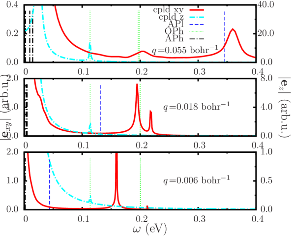
Figure 2: (color online) Amplitude of the ions’ oscillations as a function of the frequency of the applied field. Red solid line and cyan dash-dotted line are the coupled phonon-plasmon oscillations with $xy$- and $z$-polarization, respectively. The green dotted and black dash-dotted vertical lines show the positions of the optical and acoustic phonons, respectively, while the blue vertical dashed lines are the positions of the maxima of acoustic plasmon calculated with the frozen lattice.

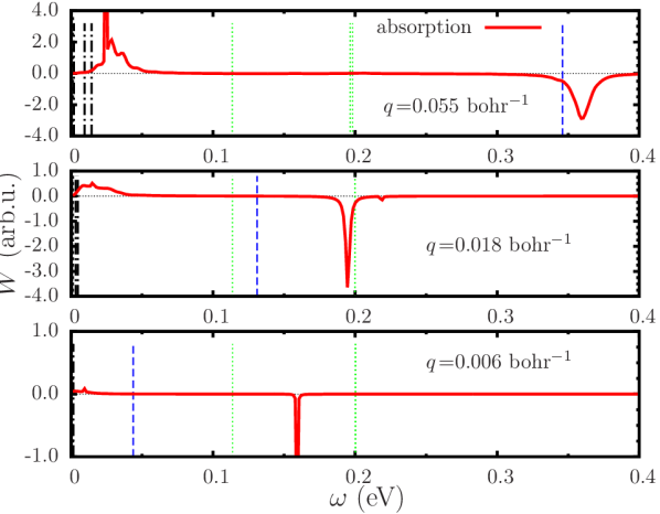
Figure 3: (color online) Energy absorption by the unit cell of the lattice per unit time (red solid line). The position of optical phonons are shown with green dotted lines, while the blue dashed lines are the positions of the maxima of acoustic-plasmon in the calculation with the frozen lattice.

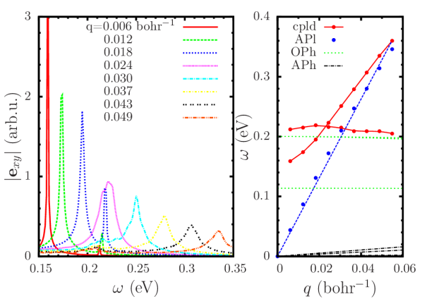
Figure 4: (color online) Dispersion of the coupled mode with the $xy$ polarization represented by the amplitude of an ion oscillation vs. the frequency $\omega$ at a number of the wave-vector $q$ values (left) and the dispersion law $\omega(q)$ (red solid lines) derived from the plots in the left panel (right). Dispersion of the optical and acoustic phonons is shown with the green dotted and black dash-dotted lines, respectively.

Figure 4, right panel, shows the $q$-vector dispersion derived from the ions’ oscillations amplitude dependence on the frequency (left panel). We conclude, that at smaller $q$-vectors, the acoustic-like linear dispersion of the coupled mode is lost, indicating that in this regime APl in graphene is an artefact of the frozen-lattice approximation. The second branch of the coupled mode remains close and above the $xy$-polarized OPh, varying non-monotonically and eventually converging to the latter.

In conclusion, we have implemented a fully dynamic (frequency-dependent density-functional perturbation theory) calculation of coupled electron-lattice oscillations in graphene. The coupled mode behaves quite differently from the individual phonon and acoustic plasmon modes, previously known in graphene, and the former replaces the two latter, as acoustic plasmons and phonons do not exist in graphene by themselves, but they constitute a unified excitation of the electronic and ionic subsystems. The coupling provides a mechanism for the transfer of energy between the electronic subsystem and the lattice, which is shown to go in both directions depending on the frequency range. From this, promising pathways of tunable heating and cooling of the lattice by the electronic subsystem can be clearly previewed.

*

Appendix A Derivation of Eq. (12)

We perform the 2D Fourier transform of Eq. (11)

$$\begin{split}\delta\phi^{I}_{b}(\mathbf{G}\!+\!\mathbf{q},z,\omega)\!=\!\frac{2\pi}{s_{0}}\!\sum\limits_{\alpha}\!Z_{\alpha}\mathbf{e}_{\alpha}\!\cdot\!\mathbf{Y}(z,\mathbf{G}\!+\!\mathbf{q})e^{-i(\mathbf{G}\!+\!\mathbf{q})\cdot\mathbf{b}_{\alpha}},\end{split}$$ (20)

where the vector function $\mathbf{Y}$ is defined by Eq. (16). Inverting Eq. (10) in the reciprocal space, we can write

$$\delta\phi(\mathbf{G}\!+\!\mathbf{q},z,\omega)=\sum\limits_{\mathbf{G}^{\prime}}\int\epsilon^{-1}_{\mathbf{G}\mathbf{G}^{\prime}}(\mathbf{q},z,z^{\prime},\omega)\times\left[\delta\phi^{\textit{ext}}(\mathbf{G}^{\prime}\!\!+\!\mathbf{q},z^{\prime},\omega)+\delta\phi^{I}_{bare}(\mathbf{G}^{\prime}\!+\!\mathbf{q},z^{\prime},\omega)\right]dz^{\prime}.$$ (21)

Then we can write for the gradient of the effective potential

$$\begin{split}&\nabla\left.\delta\phi^{\textit{eff}}_{\alpha\mathbf{0}}(\mathbf{r},\omega)\right|_{\mathbf{r}=\mathbf{b}_{\alpha}}=\sum\limits_{\mathbf{G}\mathbf{G}^{\prime}}e^{i(\mathbf{G}+\mathbf{q})\cdot\mathbf{b}_{\alpha}}\left[i(\mathbf{G}+\mathbf{q})+\hat{\mathbf{z}}\frac{\partial}{\partial z}\right]\int\left\{\epsilon^{-1}_{\mathbf{G}\mathbf{G}^{\prime}}(\mathbf{q},z^{\prime},\omega)\phi^{\textit{ext}}(\mathbf{G}^{\prime}+\mathbf{q},z^{\prime},\omega)+\frac{2\pi}{s_{0}}\times\right.\\ &\left.\sum\limits_{\beta}Z_{\beta}e^{-i(\mathbf{G}^{\prime}+\mathbf{q})\cdot\mathbf{b}_{\beta}}\!\!\int\!\left[\epsilon^{-1}_{\mathbf{G}\mathbf{G}^{\prime}}(\mathbf{q},z^{\prime},\omega)-\delta_{\mathbf{G}\mathbf{G}^{\prime}}\delta(z-z^{\prime})\right]\mathbf{e}_{\beta}\cdot\mathbf{Y}(z^{\prime},\mathbf{G}^{\prime}+\mathbf{q})\right\}_{z=0}\!\!\!\!\!\!\!dz^{\prime}\left.\!-\!\!\!\!\!\!\sum\limits_{(\beta\mathbf{R})\neq(\alpha\mathbf{0})}\!\!\!\!\!\!\!\!e^{i\mathbf{q}\cdot\mathbf{R}}\nabla(\mathbf{e}_{\beta}\!\cdot\!\nabla)\frac{Z_{\beta}}{|\mathbf{r}\!-\!\mathbf{b}_{\beta}\!-\!\mathbf{R}|}\right|_{\mathbf{r}=\mathbf{b}_{\alpha}}.\end{split}$$ (22)

We take use of the static sum-rule Nazarov et al. (2005)

$$\nabla n_{0}(\mathbf{r})=-\int\chi(\mathbf{r},\mathbf{r}^{\prime},0)\nabla^{\prime}v^{\textit{ext}}(\mathbf{r}^{\prime})\,d\mathbf{r}^{\prime}.$$ (23)

Then

$$\int\frac{\nabla n_{0}(\mathbf{r}^{\prime})}{|\mathbf{r}^{\prime}-\mathbf{r}|}d\mathbf{r}^{\prime}\!=\!\lim_{\mathbf{q}\rightarrow\mathbf{0}}\frac{2\pi}{s_{0}}\!\!\sum\limits_{\beta\mathbf{G}\mathbf{G}^{\prime}}\!Z_{\beta}\int\!\!\left[\epsilon^{-1}_{\mathbf{G}\mathbf{G}^{\prime}}(\mathbf{q},z,z^{\prime},0)-\delta_{\mathbf{G}\mathbf{G}^{\prime}}\delta(z\!-\!z^{\prime})\right]\mathbf{Y}(z^{\prime},\mathbf{G}^{\prime}+\mathbf{q})e^{i(\mathbf{G}+\mathbf{q})\cdot\mathbf{r}}e^{-i(\mathbf{G}^{\prime}+\mathbf{q})\cdot\mathbf{b}_{\beta}}dz^{\prime}.$$ (24)

Finally, we have for the force acting on the $\alpha$-th nucleus

$$F_{\alpha i}\!=\!F^{\textit{ext}}_{\alpha i}(\mathbf{q},\omega)\!+\!F^{\textit{ei}}_{\alpha i}(\mathbf{q},\omega)\!+\!\!\sum\limits_{\beta k}\!N_{\alpha i,\beta k}(\mathbf{q},\omega)e_{\beta k},$$ (25)

$$N_{\alpha i,\beta k}(\mathbf{q},\omega)=P_{\alpha i,\beta k}(\mathbf{q},\omega)-\delta_{\alpha\beta}\sum\limits_{\gamma}P_{\alpha i,\gamma k}(\mathbf{0},0),$$ (26)

where

$$F^{\textit{ext}}_{\alpha i}=-Z_{\alpha}\sum\limits_{\mathbf{G}}e^{i(\mathbf{G}+\mathbf{q})\cdot\mathbf{b}_{\alpha}}\left.\left[i(G_{i}+q_{i})+\hat{z}_{i}\frac{\partial}{\partial z}\right]\phi^{\textit{ext}}(\mathbf{G}+\mathbf{q},z,\omega)\right|_{z=0},$$ (27)

$$F^{\textit{ei}}_{\alpha i}\!=\!2\pi Z_{\alpha}\!\!\sum\limits_{\mathbf{G}\mathbf{G}^{\prime}}\int\!Y_{i}(z,\mathbf{G}+\mathbf{q})\chi_{\mathbf{G}\mathbf{G}^{\prime}}(\mathbf{q},z,z^{\prime},\omega)e^{i(\mathbf{G}\!+\!\mathbf{q})\cdot\mathbf{b}_{\alpha}}\phi^{\textit{ext}}(\mathbf{G}^{\prime}\!+\!\mathbf{q},z^{\prime},\omega)dzdz^{\prime},$$ (28)

$$P_{\alpha i,\beta k}(\mathbf{q},\omega)=Q_{\alpha i,\beta k}(\mathbf{q},\omega)+S_{\alpha i,\beta k}(\mathbf{q}),$$ (29)

$$Q_{\alpha i,\beta k}(\mathbf{q},\omega)=\frac{(2\pi)^{2}}{s_{0}}\sum\limits_{\mathbf{G}\mathbf{G}^{\prime}}Z_{\alpha}Z_{\beta}e^{i(\mathbf{G}+\mathbf{q})\cdot\mathbf{b}_{\alpha}}e^{-i(\mathbf{G}^{\prime}+\mathbf{q})\cdot\mathbf{b}_{\beta}}\int Y_{i}(z,\mathbf{G}+\mathbf{q})\chi_{\mathbf{G}\mathbf{G}^{\prime}}(\mathbf{q},z,z^{\prime},\omega)Y_{k}(z^{\prime},\mathbf{G}^{\prime}+\mathbf{q})dzdz^{\prime},$$ (30)

$$S_{\alpha i,\beta k}(\mathbf{q})\!=\!\left.\!\!\sum\limits_{\mathbf{R}}\!\left[1\!-\!\delta_{\mathbf{R}\mathbf{0}}\delta_{\beta\alpha}\right]e^{i\mathbf{q}\cdot\mathbf{R}}\nabla_{i}\nabla_{k}\frac{Z_{\alpha}Z_{\beta}}{|\mathbf{r}\!-\!\mathbf{b}_{\beta}\!-\!\mathbf{R}|}\right|_{\mathbf{r}=\mathbf{b}_{\alpha}}\!\!\!.$$ (31)

Noting that within the static approximation ($\omega=0$) our theory reduces to the conventional density-functional perturbation theory (DFPT) Giannozzi and Baroni (2005), we can conveniently rewrite Eq. (25) as Eq. (12).

References

Castro Neto et al. (2009)A. H. Castro Neto, F. Guinea,
N. M. R. Peres, K. S. Novoselov, and A. K. Geim, Rev. Mod. Phys. 81, 109 (2009).
Pisarra et al. (2013)M. Pisarra, A. Sindona,
P. Riccardi, V. M. Silkin, and J. M. Pitarke, “Acoustic plasmons in extrinsic free-standing
graphene,” (2013), arXiv:1306.6273 [cond-mat.mes-hall]
.
Pitarke et al. (2004)J. M. Pitarke, V. U. Nazarov, V. M. Silkin,
E. V. Chulkov, E. Zaremba, and P. M. Echenique, Phys.
Rev. B 70, 205403
(2004).
Giannozzi and Baroni (2005)P. Giannozzi and S. Baroni, in Handbook of
Materials Modeling, edited by S. Yip (Springer, 2005) pp. 189–208.
Bostwick et al. (2007)A. Bostwick, T. Ohta,
T. Seyller, K. Horn, and E. Rotenberg, NATURE
PHYSICS 3, 36 (2007).
Note (1)In the context of this work, the conventional term dynamic matrices contains ambiguity since, in fact, they account exactly
for the static (frequency independent) part of the force
acting on an ion.