Construction of conformal mappings by generalized polarization tensors

Abstract

We present a new systematic method to construct the conformal mapping from outside the unit disc to outside of a simply connected domain using the generalized polarization tensors. We also present some numerical results to validate effectiveness of the method.

1 Introduction

Riemann mapping theorem tells us that if the domain $\Omega$ is simply connected, then there is a conformal mapping from $\mathbb{C}\setminus U$ ($U$ is the unit disc) onto $\mathbb{C}\setminus\Omega$ of the form

$$\Phi(\zeta)=\mu_{-1}\zeta+\mu_{0}+\frac{\mu_{1}}{\zeta}+\frac{\mu_{2}}{\zeta^{2}}+\cdots,$$ (1.1)

and the mapping is unique under the assumption $\mu_{-1}>0$. The purpose of this paper is to present a new method to compute the coefficients $\mu_{-1},\mu_{0},\mu_{1},\ldots$ of the mapping.

Since the conformal mapping plays a fundamental role in various areas of mathematics and applications, many methods to construct conformal mappings have been introduced, for which we refer readers to [15] and comprehensive references therein instead of citing a long list of literature on numerical computation of the conformal mapping. The method of this paper uses the generalized polarization tensors (GPTs). The GPT is a sequence of tensors (matrices in two dimensions) associated with a domain which appears naturally in the multi-polar expansion of the electric potential. It contains rich information of the shape of the domain. For example, it is proved in [7] that the full set of GPTs determines the domain uniquely. The notion of GPTs has been used in various areas of applications such as inverse problems and imaging and the theory of composites. We refer to [8, 9, 16, 18] and references therein for these applications. More recent applications of GPT include shape representations [5, 11], dictionary matching [2, 4], invisibility cloaking [10], and electro-sensing [1, 3].

In this paper we derive canonical relations between GPTs and coefficients of the conformal mapping. Since GPTs of a domain can be computed numerically using the boundary integral method (see section 2), so can the coefficients of the conformal mapping using these relations. We will show some numerical examples of the ranges of mappings $\mu_{-1}\zeta+\mu_{0}+\frac{\mu_{1}}{\zeta}+\cdots+\frac{\mu_{n}}{\zeta^{n}}$ for $n=1,2,\ldots$. They clearly exhibit how the ranges gradually approximate the given domain.

This paper is organized as follows. In section 2 we review the definition and computation of GPT, and its relation to eigenvalues of Neumann-Poincaré operator. Section 3 is to derive the relation between GPTs and coefficients of the conformal mapping. Some numerical examples are provided in section 4. The paper is concluded with some discussions.

2 GPTs and eigenvalues of Neumann-Poincaré operator

Let $\Omega$ be a domain with the Lipschitz boundary in $\mathbb{R}^{2}$ and suppose that the conductivity (or the dielectric constant) of $\Omega$ is $k$ and that of the background is $1$ ($k\neq 1$). So, the distribution of the conductivity is given by

$$\sigma=k\chi(\Omega)+\chi(\mathbb{R}^{2}\setminus\overline{\Omega}),$$ (2.1)

where $\chi$ denotes the indicator function. For a given harmonic function $h$ in $\mathbb{R}^{2}$ we consider the following transmission problem:

$$\left\{\begin{array}[]{ll}\nabla\cdot\sigma\nabla u=0&\mbox{in }\mathbb{R}^{2},\\ \vskip 3.0pt plus 1.0pt minus 1.0pt\cr u(x)-h(x)=O(|x|^{-1})&\mbox{as }|x|\to\infty.\end{array}\right.$$ (2.2)

If $h$ takes the form in polar coordinates

$$h(x)=a_{0}+\sum_{n=1}^{\infty}r^{n}(a_{n}^{c}\cos n\theta+a_{n}^{s}\sin n\theta),$$ (2.3)

then it is known [8] that the solution $u$ to (2.2) can be represented as

$$(u-h)(x) =-\sum_{m=1}^{\infty}\frac{\cos m\theta}{2\pi mr^{m}}\sum_{n=1}^{\infty}\bigr{(}M_{mn}^{cc}a_{n}^{c}+M_{mn}^{cs}a_{n}^{s}\bigr{)}$$

$$\quad-\sum_{m=1}^{\infty}\frac{\sin m\theta}{2\pi mr^{m}}\sum_{n=1}^{\infty}\bigr{(}M_{mn}^{sc}a_{n}^{c}+M_{mn}^{ss}a_{n}^{s}\bigr{)}\quad\mbox{as }|x|\to\infty,$$ (2.4)

The quantities $M_{mn}^{\alpha\beta}$ ($\alpha,\beta=c,s$) appearing in the expansion (2.4) are called (contracted) generalized polarization tensors (GPTs).

We emphasize that GPTs can be computed numerically once the domain is given. In fact, let

$$P_{n}^{c}(x)=r^{n}\cos n\theta\quad\mbox{and}\quad P_{n}^{s}(x)=r^{n}\sin n\theta.$$ (2.5)

Then $M_{mn}^{\alpha\beta}$, $\alpha,\beta=c,s$, are given by

$$M^{\alpha\beta}_{mn}=\int_{\partial\Omega}P_{m}^{\beta}(x)(\lambda I-\mathcal{K}^{*}_{\partial\Omega})^{-1}[\nu\cdot\nabla P_{n}^{\alpha}](x)\,d\sigma,$$ (2.6)

where

$$\lambda=\frac{k+1}{2(k-1)},$$ (2.7)

and $\mathcal{K}^{*}_{\partial\Omega}$ is the Neumann-Poincaré (NP) operator defined by

$$\mathcal{K}^{*}_{\partial\Omega}[\varphi](x)=\frac{1}{2\pi}\int_{\partial\Omega}\frac{\langle x-y,\nu_{x}\rangle}{|x-y|^{2}}\varphi(y)\,d\sigma(y)\;,\quad x\in\partial\Omega.$$ (2.8)

Here $\nu_{x}$ is the outward unit normal vector to $\partial B$ at $x$. See [8, 16] for derivation of (2.6). We emphasize that $|\lambda|\geq 1/2$.

Let us look into the connection between GPTs and eigenvalues of the NP-operator (the reciprocal of the eigenvalues of the NP-operator are called the Fredholm eigenvalues). The connection between Fredholm eigenvalues and conformal mapping was investigated in [19, 20]. Let $\mathcal{S}_{\partial\Omega}[\varphi]$ be the single layer potential of a density function $\varphi\in L^{2}(\partial\Omega)$, namely,

$$\mathcal{S}_{\partial\Omega}[\varphi](x):=\frac{1}{2\pi}\int_{\partial\Omega}\ln|x-y|\varphi(y)\,d\sigma(y)\;,\quad x\in\mathbb{R}^{2}.$$ (2.9)

The relation between the boundary value of the single layer potential and the NP-operator is given by the following jump formula:

$$\frac{\partial}{\partial\nu}\mathcal{S}_{\partial\Omega}[\varphi]\big{|}_{-}(x)=\biggl{(}-\frac{1}{2}I+\mathcal{K}_{\partial\Omega}^{*}\biggr{)}[\varphi](x),\quad x\in\partial\Omega\;.$$ (2.10)

Here, $\frac{\partial}{\partial\nu}$ denotes the normal derivative and the subscript $-$ indicates the limit from the inside $\Omega$.

It is known (see, for example, [16]) that $-\langle\varphi,\mathcal{S}_{\partial\Omega}[\varphi]\rangle$ is an inner product on $L^{2}_{0}(\partial\Omega)$ which is the space of square integrable functions with the mean zero. Let $\mathcal{H}$ be the Hilbert space $L^{2}_{0}(\partial\Omega)$ equipped with this inner product, and define

$$\langle\varphi,\psi\rangle_{\mathcal{H}}:=-\langle\varphi,\mathcal{S}_{\partial\Omega}[\psi]\rangle,\quad\varphi,\psi\in\mathcal{H}.$$ (2.11)

Because of Plemelj’s symmetrization principle (also known as Calderón’s identity)

$$\mathcal{S}_{\partial\Omega}\mathcal{K}^{*}_{\partial\Omega}=\mathcal{K}_{\partial\Omega}\mathcal{S}_{\partial\Omega},$$ (2.12)

the operator $\mathcal{K}^{*}_{\partial\Omega}$ is self-adjoint on $\mathcal{H}$.

If $\partial\Omega$ is $\mathcal{C}^{1,\alpha}$ for some $\alpha>0$, then $\mathcal{K}^{*}_{\partial\Omega}$ is compact on $\mathcal{H}$. So, $\mathcal{K}^{*}_{\partial\Omega}$ has eigenvalues accumulating to $0$. Let $\lambda_{1},\lambda_{2},\ldots$ ($|\lambda_{1}|\geq|\lambda_{2}|\geq\ldots$) be eigenvalues of $\mathcal{K}^{*}_{\partial\Omega}$ on $\mathcal{H}$ counting multiplicities, and $\varphi_{1},\varphi_{2},\ldots$ be the corresponding (normalized) eigenfunctions. Then $|\lambda_{n}|<1/2$ for all $n$ and $\mathcal{K}^{*}_{\partial\Omega}$ admits the spectral resolution

$$\mathcal{K}^{*}_{\partial\Omega}=\sum_{j=1}^{\infty}\lambda_{j}\varphi_{j}\otimes\varphi_{j}$$ (2.13)

in $\mathcal{H}$. We emphasize that $\{\varphi_{j}\}$ is a basis for $\mathcal{H}$. Using (2.13), one can easily obtain that

$$M_{mn}^{\alpha\beta}=\sum_{j=1}^{\infty}\frac{\langle\nu\cdot\nabla P_{n}^{\alpha},\varphi_{j}\rangle_{\mathcal{H}}\langle P_{m}^{\beta},\varphi_{j}\rangle}{\lambda-\lambda_{j}}.$$ (2.14)

In above the second inner product is the usual inner product on $L^{2}(\partial\Omega)$. But since $\mathcal{K}^{*}_{\partial\Omega}[\varphi_{j}]=\lambda_{j}\varphi_{j}$, we have from (2.10) that

$$\frac{\partial}{\partial\nu}\mathcal{S}_{\partial\Omega}[\varphi_{j}]\big{|}_{-}=\biggl{(}-\frac{1}{2}I+\mathcal{K}_{\partial\Omega}^{*}\biggr{)}[\varphi_{j}]=\biggl{(}\lambda_{j}-\frac{1}{2}\biggr{)}\varphi_{j},$$

and hence

$$\varphi_{j}=\frac{1}{\lambda_{j}-\frac{1}{2}}\frac{\partial}{\partial\nu}\mathcal{S}_{\partial\Omega}[\varphi_{j}]\big{|}_{-}.$$

Therefore, we have

$$\langle P_{m}^{\beta},\varphi_{j}\rangle=\frac{1}{\lambda_{j}-\frac{1}{2}}\langle P_{m}^{\beta},\nu\cdot\nabla\mathcal{S}_{\partial\Omega}[\varphi_{j}]|_{-}\rangle=\frac{1}{\lambda_{j}-\frac{1}{2}}\langle\nu\cdot\nabla P_{m}^{\beta},\varphi_{j}\rangle_{\mathcal{H}},$$

where the last equality follows from the divergence theorem. So we have the following relation between GPTs and eigenvalues of NP-operator:

$$M_{mn}^{\alpha\beta}=\sum_{j=1}^{\infty}\frac{\langle\nu\cdot\nabla P_{n}^{\alpha},\varphi_{j}\rangle_{\mathcal{H}}\langle\nu\cdot\nabla P_{m}^{\beta},\varphi_{j}\rangle_{\mathcal{H}}}{(\lambda-\lambda_{j})(\lambda_{j}-\frac{1}{2})}.$$ (2.15)

We mention that if $k=0$, then $\lambda=-1/2$.

3 GPTs and conformal mappings

Suppose now that the inclusion is insulated so that $k=0$. Then, the equation (2.2) is replaced by

$$\begin{cases}\Delta u=0\quad&\mbox{in }\mathbb{R}^{2}\setminus\overline{\Omega},\\ \displaystyle\frac{\partial u}{\partial\nu}=0&\mbox{on }\partial\Omega,\\ u(x)-h(x)=O(|x|^{-1})&\mbox{as }|x|\to\infty.\end{cases}$$ (3.1)

Let $u$ be the solution to this equation, and let $H$ be an entire function such that $\Re H=h$, and $U$ be an analytic function in $\mathbb{C}\setminus\overline{\Omega}$ such that $\Re U=u$. Then $H$ takes the form

$$H(z)=\alpha_{0}+\sum_{n=1}^{\infty}\alpha_{n}z^{n},\quad\alpha_{n}=a_{n}^{c}-ia_{n}^{s},$$

and $U$ takes the form

$$U(z)=H(z)-\sum_{m=1}^{\infty}\frac{\beta_{m}}{z^{m}},$$ (3.2)

where

$$\beta_{m}:=\frac{1}{2\pi m}\sum_{n=1}^{\infty}\left[(M_{mn}^{cc}a_{n}^{c}+M_{mn}^{cs}a_{n}^{s})+i(M_{mn}^{sc}a_{n}^{c}+M_{mn}^{ss}a_{n}^{s})\right].$$ (3.3)

It is more convenient to write $\beta_{m}$ as

$$\beta_{m}=\sum_{n=1}^{\infty}(\gamma_{mn}^{1}\alpha_{n}+\gamma_{mn}^{2}\overline{\alpha_{n}})$$ (3.4)

with

$$\gamma_{mn}^{1}:=\frac{1}{4\pi m}(M_{mn}^{cc}-M_{mn}^{ss}+i(M_{mn}^{cs}+M_{mn}^{sc})),$$ (3.5)

$$\gamma_{mn}^{2}:=\frac{1}{4\pi m}(M_{mn}^{cc}+M_{mn}^{ss}-i(M_{mn}^{cs}-M_{mn}^{sc})).$$ (3.6)

Then $U$ can be written as

$$U(z)=\alpha_{0}+\sum_{n=1}^{\infty}\left(\alpha_{n}z^{n}-\sum_{m=1}^{\infty}\frac{\gamma_{mn}^{1}\alpha_{n}+\gamma_{mn}^{2}\overline{\alpha_{n}}}{z^{m}}\right).$$ (3.7)

So, we have

$$U(z)=\alpha_{0}+\sum_{n=1}^{\infty}\left[a_{n}^{c}\left(z^{n}-\sum_{m=1}^{\infty}\frac{\gamma_{mn}^{1}+\gamma_{mn}^{2}}{z^{m}}\right)-ia_{n}^{s}\left(z^{n}-\sum_{m=1}^{\infty}\frac{\gamma_{mn}^{1}-\gamma_{mn}^{2}}{z^{m}}\right)\right].$$ (3.8)

One can easily see from the Cauchy-Riemann equation that the boundary condition $\frac{\partial u}{\partial\nu}=0$ in (3.1) is equivalent to

$$\Im U=\mbox{constant}\quad\mbox{on }\partial\Omega.$$ (3.9)

Since this condition holds for any entire function $H$, we infer from (3.8) that

$$\Re\left(z^{n}-\sum_{m=1}^{\infty}\frac{\gamma_{mn}^{1}-\gamma_{mn}^{2}}{z^{m}}\right)=\mbox{const.},\quad\Im\left(z^{n}-\sum_{m=1}^{\infty}\frac{\gamma_{mn}^{1}+\gamma_{mn}^{2}}{z^{m}}\right)=\mbox{const.}$$ (3.10)

on $\partial\Omega$ for every positive integer $n$.

Let $z=\Phi(\zeta)$ be the conformal mapping from $|\zeta|>1$ onto $\mathbb{C}\setminus\overline{\Omega}$, given by (1.1). Let us write $c=\mu_{-1}$ for ease of notation. Then $U\circ\Phi(\zeta)$ is analytic in $|\zeta|>1$ and takes the form

$$U\circ\Phi(\zeta) =\alpha_{0}+\sum_{n=1}^{\infty}\left(\alpha_{n}\Phi(\zeta)^{n}-\sum_{m=1}^{\infty}\frac{\gamma_{mn}^{1}\alpha_{n}+\gamma_{mn}^{2}\overline{\alpha_{n}}}{\Phi(\zeta)^{m}}\right).$$ (3.11)

We infer from (3.10) that

$$\Re\left(\Phi(\zeta)^{n}-\sum_{m=1}^{\infty}\frac{\gamma_{mn}^{1}-\gamma_{mn}^{2}}{\Phi(\zeta)^{m}}\right)=\mbox{constant on }|\zeta|=1$$ (3.12)

and

$$\Im\left(\Phi(\zeta)^{n}-\sum_{m=1}^{\infty}\frac{\gamma_{mn}^{1}+\gamma_{mn}^{2}}{\Phi(\zeta)^{m}}\right)=\mbox{constant on }|\zeta|=1.$$ (3.13)

These conditions implies that

$$\Phi(\zeta)^{n}-\sum_{m=1}^{\infty}\frac{\gamma_{mn}^{1}}{\Phi(\zeta)^{m}}+\overline{\sum_{m=1}^{\infty}\frac{\gamma_{mn}^{2}}{\Phi(\zeta)^{m}}}$$ (3.14)

is constant on $|\zeta|=1$. Since $\sum_{m=1}^{\infty}\frac{\gamma_{mn}^{2}}{\Phi(\zeta)^{m}}$ can be expanded as

$$\sum_{m=1}^{\infty}\frac{\gamma_{mn}^{2}}{\Phi(\zeta)^{m}}=\sum_{k=1}^{\infty}\frac{s_{n}}{\zeta^{n}},\quad|\zeta|>1,$$ (3.15)

it follows from (3.14) that

$$\Phi(\zeta)^{n}-\sum_{m=1}^{\infty}\frac{\gamma_{mn}^{1}}{\Phi(\zeta)^{m}}=\mbox{constant}-\sum_{k=1}^{\infty}\bar{s}_{n}\zeta^{n},\quad|\zeta|=1,$$ (3.16)

so that

$$\Phi(\zeta)^{n}-\sum_{m=1}^{\infty}\frac{\gamma_{mn}^{1}}{\Phi(\zeta)^{m}}\quad\mbox{is an entire function}.$$ (3.17)

We now derive relations among GPTs and coefficients of the conformal mapping using (3.13) and (3.17). We observe, for $\zeta$ with large modulus,

$$\frac{1}{\Phi(\zeta)} =\frac{1}{c\zeta}\cdot\frac{1}{1+\frac{\mu_{0}}{c\zeta}+\frac{\mu_{1}}{c\zeta^{2}}+\frac{\mu_{2}}{c\zeta^{3}}+\ldots}$$

$$=\frac{1}{c\zeta}\sum_{j=0}^{\infty}(-1)^{j}\left(\frac{\mu_{0}}{c\zeta}+\frac{\mu_{1}}{c\zeta^{2}}+\frac{\mu_{2}}{c\zeta^{3}}+\ldots\right)^{j}=\sum_{k=1}^{\infty}\frac{B_{k}}{\zeta^{k}},$$ (3.18)

where $B_{1}=1/c$ and

$$B_{k}:=\frac{1}{c}\sum_{s_{1}k_{1}+\ldots+s_{j}k_{j}=k-1\atop s_{1},\ldots,s_{j}>0,~{}k_{j}>\ldots>k_{1}>0}\left(\frac{-1}{c}\right)^{s_{1}+\ldots+s_{j}}\frac{(s_{1}+\ldots+s_{j})!}{s_{1}!\cdots s_{j}!}{\mu_{k_{1}-1}^{s_{1}}\cdots\mu_{k_{j}-1}^{s_{j}}},\quad k\geq 2.$$ (3.19)

We emphasize that $B_{k}$ ($k\geq 2$) is determined by $\mu_{\ell}$ for $\ell\leq k-2$. It is helpful to write down first few terms:

$$B_{2} =-\mu_{0}/c^{2},$$

$$B_{3} =-\mu_{1}/c^{2}+\mu_{0}^{2}/c^{3},$$

$$B_{4} =-\mu_{2}/c^{2}+2\mu_{0}\mu_{1}/c^{3}-\mu_{0}^{3}/c^{4},$$ (3.20)

$$B_{5} =-\mu_{3}/c^{2}+\mu_{1}^{2}/c^{3}+2\mu_{0}\mu_{2}/c^{3}-3\mu_{0}^{2}\mu_{1}/c^{4}+\mu_{0}^{4}/c^{5},$$

$$B_{6} =-\mu_{4}/c^{2}+2\mu_{0}\mu_{3}/c^{3}+2\mu_{1}\mu_{2}/c^{3}-3\mu_{0}\mu_{1}^{2}/c^{4}-\mu_{0}^{5}/c^{6}.$$

We now consider the conditions (3.17) when $n=1$. One can see from (3.18) that

$$\sum_{m=1}^{\infty}\frac{\gamma_{m1}^{1}}{\Phi(\zeta)^{m}}=\sum_{\ell=1}^{\infty}\sum_{s_{1}n_{1}+\ldots+s_{j}n_{j}=\ell\atop s_{1},\ldots,s_{j}>0,~{}n_{j}>\ldots>n_{1}>0}\gamma_{s_{1}+\ldots+s_{j},1}^{1}\frac{(s_{1}+\ldots+s_{j})!}{s_{1}!\cdots s_{j}!}\frac{B_{n_{1}}^{s_{1}}\cdots B_{n_{j}}^{s_{j}}}{\zeta^{\ell}},$$

and hence

$$\Phi(\zeta)-\sum_{m=1}^{\infty}\frac{\gamma_{m1}^{1}}{\Phi(\zeta)^{m}}$$

$$=c\zeta+\sum_{\ell=0}^{\infty}\frac{\mu_{\ell}}{\zeta^{\ell}}-\sum_{\ell=1}^{\infty}\frac{1}{\zeta^{\ell}}\sum_{s_{1}n_{1}+\ldots+s_{j}n_{j}=\ell\atop s_{1},\ldots,s_{j}>0,~{}n_{j}>\ldots>n_{1}>0}\gamma_{s_{1}+\ldots+s_{j},1}^{1}\frac{(s_{1}+\ldots+s_{j})!}{s_{1}!\cdots s_{j}!}B_{n_{1}}^{s_{1}}\cdots B_{n_{j}}^{s_{j}}.$$ (3.21)

It then follows from (3.17) that

$$\mu_{\ell}=\sum_{s_{1}n_{1}+\ldots+s_{j}n_{j}=\ell\atop s_{1},\ldots,s_{j}>0,~{}n_{j}>\ldots>n_{1}>0}\gamma_{s_{1}+\ldots+s_{j},1}^{1}\frac{(s_{1}+\ldots+s_{j})!}{s_{1}!\cdots s_{j}!}B_{n_{1}}^{s_{1}}\cdots B_{n_{j}}^{s_{j}},\quad\ell\geq 1.$$ (3.22)

We note that $\mu_{\ell}$ is determined by $\gamma_{m1}^{1}$ for $m\leq\ell$ and $B_{k}$ for $k\leq\ell$ which in turn determined by $\mu_{j}$ for $j\leq k-2$ as we have seen it in (3.19). So, $\mu_{\ell}$ ($\ell\geq 1$) is determined by $\gamma_{m1}^{1}$ for $m\leq\ell$ and $\mu_{0},\ldots,\mu_{\ell-2}$ ($\mu_{-1}=c$). For example, we have first few terms as follows:

$$\mu_{1} =\gamma_{11}^{1}B_{1},$$

$$\mu_{2} =\gamma_{21}^{1}B_{1}^{2}+\gamma_{11}^{1}B_{2},$$

$$\mu_{3} =\gamma_{31}^{1}B_{1}^{3}+2\gamma_{21}^{1}B_{1}B_{2}+\gamma_{11}^{1}B_{3},$$ (3.23)

$$\mu_{4} =\gamma_{41}^{1}B_{1}^{4}+\gamma_{21}B_{2}^{2}+3\gamma_{31}^{1}B_{1}^{2}B_{2}+2\gamma_{21}^{1}B_{1}B_{3}+\gamma_{11}^{1}B_{4},$$

$$\mu_{5} =\gamma_{51}^{1}B_{1}^{5}+3\gamma_{31}^{1}B_{1}B_{2}^{2}+2\gamma_{21}(B_{1}B_{4}+B_{2}B_{3})+\gamma_{11}^{1}B_{5},$$

$$\mu_{6} =\gamma_{61}^{1}B_{1}^{6}+\gamma_{51}^{1}B_{1}^{4}B_{2}+\gamma_{41}^{1}B_{1}^{3}B_{3}+\gamma_{31}^{1}(B_{1}^{4}B_{4}+B_{1}B_{2}B_{3})+\gamma_{21}^{1}(B_{1}B_{5}+B_{2}B_{4}).$$

We now look into the condition (3.13) for $n=1$. One can check that

$$\Phi(\zeta)-\sum_{m=1}^{\infty}\frac{\gamma_{m1}^{1}-\gamma_{m1}^{2}}{\Phi(\zeta)^{m}}$$

$$=c\zeta+\sum_{\ell=0}^{\infty}\frac{\mu_{\ell}}{\zeta^{\ell}}-\sum_{\ell=1}^{\infty}\sum_{s_{1}n_{1}+\ldots+s_{j}n_{j}=\ell\atop s_{1},\ldots,s_{j}>0,~{}n_{j}>\ldots>n_{1}>0}(\gamma_{s_{1}+\ldots+s_{j},1}^{1}-\gamma_{s_{1}+\ldots+s_{j},1}^{2})\frac{(s_{1}+\ldots+s_{j})!}{s_{1}!\cdots s_{j}!}\frac{B_{n_{1}}^{s_{1}}\cdots B_{n_{j}}^{s_{j}}}{\zeta^{\ell}}$$

$$=c\zeta+\mu_{0}+\frac{\mu_{1}-(\gamma_{11}^{1}-\gamma_{11}^{2})/c}{\zeta}+\frac{\mu_{2}+\mu_{0}(\gamma_{11}^{1}-\gamma_{11}^{2})/c^{2}-(\gamma_{21}^{1}-\gamma_{21}^{2})/c^{2}}{\zeta^{2}}+\ldots$$ (3.24)

Then using (3.13) we obtain

$$c^{2}=-\gamma_{11}^{2},\quad\mu_{0}=-c^{-2}\gamma_{21}^{2},$$ (3.25)

and

$$\sum_{s_{1}n_{1}+\ldots+s_{j}n_{j}=\ell\atop s_{1},\ldots,s_{j}>0,~{}n_{j}>,\ldots>n_{1}>0}\gamma_{s_{1}+\ldots+s_{j},1}^{2}\frac{(s_{1}+\ldots+s_{j})!}{s_{1}!\cdots s_{j}!}B_{n_{1}}^{s_{1}}\cdots B_{n_{j}}^{s_{j}}=0,\quad\ell\geq 2.$$ (3.26)

So we conclude that all the coefficients of the conformal mapping is determined from

$$\gamma_{11}^{2},~{}\gamma_{21}^{2},~{}\{\gamma_{m1}^{1}\}_{m\in\mathbb{N}}.$$ (3.27)

In fact, $\mu_{\ell}$ can be determined inductively using these GPTs: $\mu_{-1}=c$ and $\mu_{0}$ are determined by the formula (3.25), $\mu_{1}$ is determined by the first equation in (3.23), $\mu_{\ell}$ for $\ell\geq 2$ is determined by formula (3.19) and (3.22) in terms of $\gamma_{m1}^{1}$ for $m\leq\ell$ and $\mu_{k}$ for $k\leq\ell-2$.

4 Numerical illustration

In this section we provide numerical examples of conformal mapping (1.1) to outside of simply connected domains obtained using the method presented in the previous section. In order to acquire the GPTs, we solve the boundary integral equation (2.6) numerically. We refer readers to [6] for more details of the computation and numerical codes. The number of nodal points used on $\partial\Omega$ is 3072 in each example.

Once GPTs of the given domain are computed, then the first two coefficients $\mu_{-1}$ and $\mu_{0}$ of the conformal mapping $\Phi$ are determined by (3.25), and those of higher order terms by (3.22). Let $\Phi_{N}$, $N\geq 1$, be the truncation of $\Phi$ at the $N$-th order, namely,

$$\Phi_{N}(\zeta)=\mu_{-1}\zeta+\mu_{0}+\frac{\mu_{1}}{\zeta}+\frac{\mu_{2}}{\zeta^{2}}+\cdots+\frac{\mu_{N}}{\zeta^{N}}.$$ (4.1)

In the following examples, we show the images (in black curves) of the unit circle $(S^{1})$ under the $\Phi_{N}$ for domains $\Omega$ of various shapes. The gray curves are actual boundaries of the domains.

Example 1. For ellipses, $\Phi_{1}(S^{1})$ exactly matches with the boundary of $\Omega$. See Figure 4.1. For a perturbed ellipse, $\Phi_{N}$ with $N=2$ recovers a good approximation of $\partial\Omega$.

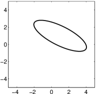
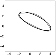
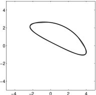
Figure 4.1: In the first figure, $\Omega$ is an ellipse and $N=1$. In the next two figures, $\Omega$ is a perturbed ellipse, and $N$ is 1 and 2 in the middle and the right figures, respectively.

Example 2. Figure 4.2 shows $\Phi_{N}(S^{1})$ is gradually changing to the boundary of a kite shape domain $\Omega$ as $N$ increases. The computed values of coefficients are presented in Table 1. The ellipse in the first figure (top left) is called the equivalent ellipse of $\Omega$ [8, 12].

$l$	-1	0	1	2	3	4	5	6
$\mu_{l}$	1.1337	-0.2415	0.1442	-0.2645	-0.1328	-0.0812	-0.0548	-0.0394

Table 1: The coefficients $\mu_{l}$, $l\leq 6$, for $\Omega$ in Figure 4.2.

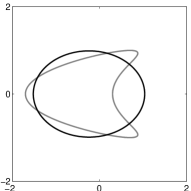
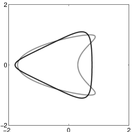
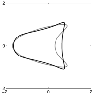
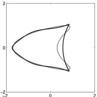
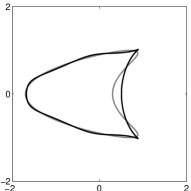
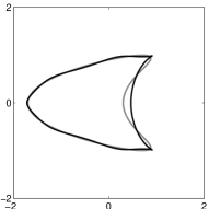
Figure 4.2: A kite-shape domain $\Omega$ and $\Phi_{N}(S^{1})$ for $N=1,\ldots,6$.

Example 3 Figure 4.3 reveals that the boundary with mild oscillation can be recovered by $\Phi_{N}$ for relatively small $N$, while that with high oscillation requires $\Phi_{N}$ for higher $N$. This fact was also observed in [11].

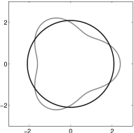
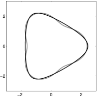
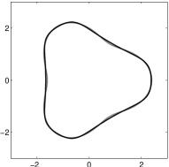
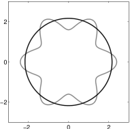
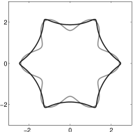
Figure 4.3: The gray curve is $\partial\Omega$ given by $r=(2+0.4\cos(p\theta))$ in polar coordinates for $p=3$ (in the top row) and $p=6$ (in the bottom), and the black is the images of the unit circle under $\Phi_{N}$ for $N=1,2,5$.

5 Further discussion

We have derived an explicit connection between GPTs and coefficients of the conformal mapping, and show by numerical examples that first few terms of the conformal mapping approximate the domain quite well.

It is quite interesting to extend results of this paper to construction of conformal mappings of multiply connected domains. We emphasize that GPTs are defined for multiply connected domains as well. In this regard, it is worth emphasizing that only the relations for $n=1$ in (3.17) and some partial relations in (3.13) are used to derive relation between GPTs and the conformal mapping. So, the relations for $n\geq 2$ and other relations in (3.13) provide relations among GPTs. In particular, the equation (3.26) says that all the terms in $\{\gamma_{m1}^{2}:~{}m\geq 3\}$ can be calculated by (3.27). For instance, we obtain

$$\gamma_{31}^{2}=\gamma_{11}^{1}\gamma_{11}^{2}+\frac{(\gamma_{21}^{2})^{2}}{\gamma_{11}^{2}}.$$ (5.1)

This relation holds only for simply connected domains. For example, if the domain is two disjoint unit disks centered at $(\pm 2,0)$, then $\gamma_{31}^{2}=-8.03$ and $\gamma_{11}^{1}\gamma_{11}^{2}+(\gamma_{21}^{2})^{2}/\gamma_{11}^{2}=-0.25.$

Note that translation, rotation, and scaling of the domain $\Omega$ are expressed as $\alpha\Phi+\beta$ for some complex numbers $\alpha$ and $\beta$. So, the quantities $\mu_{j}/\mu_{-1}$ ($j=1,2,\ldots$) are invariant under translation, rotation, and scaling. In other words, they can be used as shape descriptors in 2D, which can be computed using GPTs. It is worth mentioning that invariant shape descriptors are derived in two and three dimensions using GPTs in [2, 4] and used effectively in a new development of electro-sensing [3].

It is a classical subject to derive optimal bounds for the coefficients of the conformal mapping (see, for instance, [15] and references therein). In this regards, it is worthwhile to mention the Bieberbach conjecture and its resolution by de Brange [14]. On the other hand, it is an important problem to derive optimal bounds of GPTs. For example, the bounds for the first order GPTs ($\gamma^{1}_{11}$ and $\gamma^{2}_{11}$) are obtained in [13, 17]. The relation between GPTs and the conformal mapping obtained in this paper may shed new light on this problem.

References

• [1] H. Ammari, T. Boulier, and J. Garnier, Modeling active electrolocation in weakly electric fish, SIAM J. Imaging Sciences 6 (2013), 285–321.
• [2] H. Ammari, T. Boulier, J. Garnier, W. Jing, H. Kang and H. Wang, Target identification using dictionary matching of generalized polarization tensors, Found. Comp. Math., to appear, arXiv:1212.3544.
• [3] H. Ammari, T. Boulier, J. Garnier, and H. Wang, Shape recognition and classification in electro-sensing, submitted.
• [4] H. Ammari, D. Chung, H. Kang, and H. Wang, Invariance properties of generalized polarization tensors and design of shape descriptors in three dimensions, submitted, arXiv 1212.3519.
• [5] H. Ammari, J. Garnier, H. Kang, M. Lim, and S. Yu, Generalized polarization tensors for shape description, Numerische Math., to appear.
• [6] H. Ammri, J. Garnier, W. Jing, H. Kang, M. Lim, K. Solna, and H. Wang, Mathematical and statistical methods for multistatic imaging, Lecture Notes in Math. 2098, Springer, to appear.
• [7] H. Ammari and H. Kang, Properties of the generalized polarization tensors, SIAM J. Multiscale Modeling and Simulation 1 (2003), 335–348.
• [8] H. Ammari and H. Kang, Polarization and moment tensors with applications to inverse problems and effective medium theory, Applied Mathematical Sciences, Vol. 162, Springer-Verlag, New York, 2007.
• [9] H. Ammari and H. Kang, Expansion methods, Handbook of Mathematical Methods of Imaging, 447-499, Springer, 2011.
• [10] H. Ammari, H. Kang, H. Lee, and M. Lim, Enhancement of near cloaking using gen- eralized polarization tensors vanishing structures. Part I: The conductivity problem, Comm. Math. Phys. 317 (2013), 253–266.
• [11] H. Ammari, H. Kang, M. Lim, and H. Zribi, The generalized polarization tensors for resolved imaging. Part I: Shape reconstruction of a conductivity inclusion, Math. Comp. 81 (2012), 367–386.
• [12] M. Brühl, M. Hanke, and M.S. Vogelius, A direct impedance tomography algorithm for locating small inhomogeneities, Numer. Math. 93 (2003), 635–654.
• [13] Y. Capdeboscq and M.S. Vogelius, Optimal asymptotic estimates for the volume of in- ternal inhomogeneities in terms of multiple boundary measurements, Math. Modelling Num. Anal. 37 (2003), 227–240.
• [14] L. de Branges, A proof of the Bieberbach conjecture, Acta Math. 154 (1985), 137–152.
• [15] P. Henrici, Applied and computational complex analysis, Vol 3, John Wiley & Sons, New York, 1993.
• [16] H. Kang, Layer potential approaches to interface problems, a chapter in Inverse problems and imaging, Panoramas et Syntheses, Societe Mathematique de France, to appear.
• [17] R. Lipton, Inequalities for electric and elastic polarization tensors with applications to random composites, J. Mech. Phys. Solids 41 (1993), 809–833.
• [18] G.W. Milton, The Theory of Composites, Cambridge Monographs on Applied and Computational Mathematics, Cambridge University Press, 2002.
• [19] M. Schiffer, The Fredholm eigenvalues of plane domains, Pacific J. Math. 7 (1957), 1187–1225.
• [20] M. Schiffer, Fredholm eigenvalues and conformal mappings, Rend. Mat. e Appl. 22 (1963), 447–468.