Criteria for genuine $N$-partite continuous-variable entanglement and Einstein-Podolsky-Rosen steering

Abstract

Following previous work, we distinguish between genuine $N$-partite entanglement and full $N$-partite inseparability. Accordingly, we derive criteria to detect genuine multipartite entanglement using continuous variable (position and momentum) measurements. Our criteria are similar but different to those based on the van Loock-Furusawa inequalities, which detect full $N$-partite inseparability. We explain how the criteria can be used to detect the genuine $N$-partite entanglement of continuous variable states generated from squeezed and vacuum state inputs, including the continuous variable Greenberger-Horne-Zeilinger state, with explicit predictions for up to $N=9$. This makes our work accessible to experiment. For $N=3$, we also present criteria for tripartite Einstein-Podolsky-Rosen (EPR) steering. These criteria provide a means to demonstrate a genuine three-party EPR paradox, in which any single party is steerable by the remaining two parties.

I Introduction

There has been strong motivation to create and detect quantum states that have many atoms wine , photons, 6dicke ; svetexp ; shalm-1 or modes aokicv ; seiji ; threecolourcv entangled. Beyond the importance to the field of quantum information, such states provide evidence for mesoscopic quantum mechanics ghz ; seevinck ; svetlichny ; collins localnonlocal-2 . In any such experiment, it is essential that one can clearly distinguish the genuine $N$-partite entanglement of $N$ systems from the entanglement produced by mixing quantum states with fewer than $N$ systems entangled.

Three systems labeled $1$, $2$, and $3$ are said to be genuinely tripartite entangled iff the density operator for the tripartite system cannot be represented in the biseparable form bancalgendient ; guh4

$$\rho_{BS} = P_{1}\sum_{R}\eta_{R}^{(1)}\rho_{23}^{R}\rho_{1}^{R}+P_{2}\sum_{R^{\prime}}\eta_{R^{\prime}}^{(2)}\rho_{13}^{R^{\prime}}\rho_{2}^{R^{\prime}}$$ (1)

$$+P_{3}\sum_{R^{\prime\prime}}\eta_{R^{\prime\prime}}^{(3)}\rho_{12}^{R^{\prime\prime}}\rho_{3}^{R^{\prime\prime}},$$

where $\sum_{k=1}^{3}P_{k}=1$ and $\sum_{R}\eta_{R}^{(k)}=1$. Here, $\rho_{k}^{R}$ is an arbitrary quantum density operator for the system $k$, while $\rho_{mn}^{R}$ is an arbitrary quantum density operator for the two systems $m$ and $n$ ($k,m,n$ $\in\{1,2,3\}$). Thus, for a system described by the biseparable state $\rho_{mn}^{R}\rho_{k}^{R}$, the systems $m$ and $n$ can be bipartite entangled, but there is no entanglement between $m$ and $k$, or $n$ and $k$. Similarly, $N$ parties are “genuinely $N$-partite entangled” if all the possible biseparable mixtures describing the $N$ parties are negated.

In this paper, we use the above definition to derive criteria sufficient to confirm the genuine $N$-partite entanglement of $N$ systems, as detected by continuous variable (CV) measurements, i.e., measurements of position and momentum, or quadrature phase amplitudes. An application of the criteria would be to witness the genuine entanglement of $N$ spatially separated optical field modes aokicv ; seiji ; threecolourcv .

The continuous variable (CV) case is an important one cv gaussrmp ; rmp-1 ; slbvl rmp ; eisertplenio . CV entanglement has significant applications to quantum information technology, providing efficient deterministic teleportation tele and secure communication cry . Moreover, CV entanglement can give efficiently detected Einstein-Podolsky-Rosen correlations rmp-1 ; ou epr-1 and evidence of the entanglement of multiple macroscopic systems, consisting of many photons cv large . The CV criteria can also be applied to optomechanics, as a means to demonstrate the entanglement of three or more mechanical harmonic oscillators optmehc .

In order to claim genuine multipartite entanglement, it is necessary to falsify all mixtures of the bipartitions as in Eq. (1), as opposed to negating that the system can be in any single one of them. As pointed out by Shalm et al. shalm-1 , this leads to two definitions $-$ genuine $N$-paritite entanglement and full $N$-partite inseparability$-$ that have often been used interchangeably in the literature but in fact mean different things. This distinction for Gaussian states was also made by Hyllus and Eisert hyllus and eisert . In realistic experimental scenarios where one cannot assume pure states, the task of detecting genuine continuous variable (CV) multipartite entanglement poses a greater challenge than detecting full multipartite inseparability. This means that detecting genuine tripartite entanglement in the CV regime is more difficult than has often been supposed. Most CV criteria that have been applied to experiments assume Gaussian states Gaussian gencv ; gausadesso , or else do not in fact negate all mixtures of bipartitions (1), and thus detect full multipartite inseparability, rather than genuine multipartite entanglement cvsig ; aokicv ; seiji ; threecolourcv .

One exception is the work of Shalm et al. shalm-1 . These authors derive new CV criteria involving position and momentum observables. Shalm et al. then adapt the criteria, to demonstrate the genuine tripartite entanglement of three spatially separated photons using energy-time measurements. A second exception is Armstrong et al. seiji2 , who derive a different criterion that is used to confirm the genuine CV tripartite entanglement of three optical modes. Also, the recent work of He and Reid genepr gives criteria for genuine tripartite EPR steering, which is a special type of tripartite entanglement.

Here, we present criteria for the detection of CV multipartite entanglement. The criteria can be applied to the CV Greenberger-Horne-Zeilinger (GHZ) states braunghz that have been generated in the experiments of Aoki et al. aokicv , or the similar multipartite Einstein-Podolsky-Rosen (EPR) entangled states generated in the experiments of Armstrong et al. seiji . In Secs. II and III, we present the necessary background, and in Secs. IV and V derive criteria for the tripartite $N=3$ case. In Sec. VIII, we provide algorithms for arbitrary $N$, and give explicit predictions for up to $N=9$ modes, for the multi-mode CV GHZ- and EPR-type entangled states. The effect of transmission losses is also analyzed, in Sec. VII. Our criteria are based on the assumption that the quantum uncertainty relations for position and momentum apply to the measurements made on each system, and are not restricted to pure or mixed Gaussian states.

In Sec. VI, we analyze and derive criteria for “genuine tripartite EPR steering” genepr . “EPR steering” is the form of quantum nonlocality introduced by EPR in their paradox of 1935 epr ; hw-1 . The term “steering” was introduced by Schrodinger to describe the nonlocality highlighted by the paradox. EPR steering and the EPR paradox were realized for CV measurements in the experiment of Ou et al. ou epr-1 , based on the predictions explained in Ref. rmp-1 . In short, verification of steering amounts to a verification of entanglement, in a scenario where not all of the experimentalists can be trusted to carry out the measurements properly hw-1 ; cv trust . This is an important consideration in device-independent quantum cryptography one-sidedcrytpt . The criteria developed in this paper are likely to be useful to multiparty quantum cryptography protocols, such as quantum secret sharing secretshare .

The inequalities that we use to detect genuine $N$-partite entanglement are similar to the van Loock-Furusawa inequalities cvsig . The van Loock-Furusawa inequalities are widely used, but are designed to test for full multipartite inseparability, rather then genuine multipartite entanglement. However, we show that one of the van Loock-Furusawa inequalities will suffice to detect genuine tripartite entanglement, and that tripartite entanglement and steering can be detected for sufficient violation of other van Loock-Furusawa inequalities that are used together as a set. Our work extends beyond the $N=3$ case. We prove in Section VIII a general approach for deriving entanglement criteria based on summation of inequalities that can negate each pure biseparable state. Further, we establish that the genuine $N$-partite entanglement of CV GHZ and certain multipartite EPR states can be detected using a single suitably-optimized inequality.

II Distinguishing between genuine $N$-partite entanglement and full $N$-partite inseparability

The aim of this paper is to derive inequalities based on the assumption (1) of the biseparable mixture, and the $N$-party extensions. The violation of these inequalities will then demonstrate genuine tripartite entanglement, and, in the $N$-party case, genuine $N$-partite entanglement. First, we explain the difference between genuine $N$-paritite entanglement and full $N$-partite inseparability.

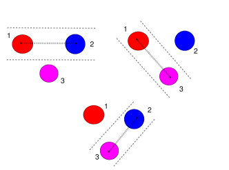
Figure 1: (Color online) Schematic of the possible biseparable quantum states for three systems, labeled $1,2,3$. Going clockwise from top left, the biseparable states are $\rho_{12,3}$, $\rho_{13,2}$, and $\rho_{23,1}$ (associated with bipartitions $12-3$, $13-2$, and $23-1$, respectively).

We consider the three-party system described by

$$\rho_{km,n}=\sum_{R}\eta_{R}^{(n)}\rho_{km}^{R}\rho_{n}^{R}$$ (2)

where two but not three of the systems can be entangled. In this notation, the $k,m,n$ denote three distinct systems, which in this paper will be modes representing an optical field or a quantized harmonic oscillator. The density operator $\rho_{km}^{R}$ can represent any quantum state for the two modes $k$ and $m$, and can account for entanglement between them. We denote the bipartition associated with the biseparable density operator $\rho_{km}^{R}\rho_{n}^{R}$ (and $\rho_{km,n}$) by $km-n$. The bipartitions for $N=3$ parties are depicted graphically in Fig. 1.

We suppose that each system is a single mode with boson operator $a_{j}$ ($j=1,2,3$) and define the quadrature amplitudes as $x_{j}=(a_{j}+a_{j}^{\dagger})$ and $p_{j}=(a_{j}-a_{j}^{\dagger})/i$. Assuming the Heisenberg uncertainty relation $\Delta x_{j}\Delta p_{j}\geq 1$, the separability assumption of (2) implies the following sum and product inequalities:

$$(\Delta u)^{2}+(\Delta v)^{2}\geq 2(|h_{n}g_{n}|+|h_{k}g_{k}+h_{m}g_{m}|)$$ (3)

and

$$\Delta u\Delta v\geq|h_{n}g_{n}|+|h_{k}g_{k}+h_{m}g_{m}|,$$ (4)

where $u=h_{n}x_{n}+h_{k}x_{k}+h_{m}x_{m}$ and $v=g_{n}p_{n}+g_{k}p_{k}+g_{m}p_{m}$. Here, $(\Delta x)^{2}$ denotes the variance of the quantum observable $x$. The sum inequality was derived by van Loock and Furusawa cvsig . The product inequality is proved in the Appendix, and is stronger, in that it will always imply the sum inequality (note the simple identity $x^{2}+y^{2}\geq 2xy$, that holds for any real numbers $x$ and $y$).

In their paper, van Loock and Furusawa consider the three inequalities

$$B_{I}\equiv[\Delta(x_{1}-x_{2})]^{2}+[\Delta(p_{1}+p_{2}+g_{3}p_{3})]^{2} \geq 4,$$

$$B_{II}\equiv[\Delta(x_{2}-x_{3})]^{2}+[\Delta(g_{1}p_{1}+p_{2}+p_{3})]^{2} \geq 4,$$

$$B_{III}\equiv[\Delta(x_{1}-x_{3})]^{2}+[\Delta(p_{1}+g_{2}p_{2}+p_{3})]^{2} \geq 4,$$

which are defined for arbitrary real parameters $g_{1}$, $g_{2}$, and $g_{3}$. They point out, using Eq. (3), that inequality $B_{I}\geq 4$ is implied by both the biseparable states $\rho_{13,2}$ and $\rho_{23,1}$, which give separability between systems $1$ and $2$. Similarly, the second inequality $B_{II}\geq 4$ is implied by the biseparable states $\rho_{13,2}$ and $\rho_{12,3}$, while the third inequality $B_{III}\geq 4$ follows from biseparable states $\rho_{12,3}$ and $\rho_{23,1}$.

In this way, van Loock and Furusawa show that the violation of any two of the inequalities of Eq. (LABEL:eq:threeineq) is sufficient to rule out that the system is described by any of the biseparable states $\rho_{12,3}$, $\rho_{13,2}$, or $\rho_{23,1}$. This result has been used in experimental scenarios aokicv ; seiji to give evidence of a “fully inseparable tripartite entangled state”. However, violating any two of the van Loock-Furusawa inequalities is not in itself sufficient to confirm genuine tripartite entanglement, as can be verified by the mixed state example given in the Appendix 4. The reason is that inequalities ruling out any of the simpler cases of Eq. (2) do not rule out the general biseparable case of Eq. (1) which considers mixtures of the different bipartitions, $\rho_{12,3}$, $\rho_{13,2}$, or $\rho_{23,1}$.

This point has been noted by Hyllus and Eisert hyllus and eisert and Shalm et al. shalm-1 and leads to two definitions in connection with multipartite entanglement. For pure states, the two definitions coincide, since a pure system cannot be in a mixture of states. For experimental verification however, an unambiguous signature of genuine tripartite entanglement becomes necessary, since one cannot assume pure states.

Before continuing, it is useful to derive the product version of the van Loock-Furusawa inequalities, that are based on the product uncertainty relation given by Eq. (4). We define:

$$S_{I}\equiv\Delta(x_{1}-x_{2})\Delta(p_{1}+p_{2}+g_{3}p_{3}) \geq 2,$$

$$S_{II}\equiv\Delta(x_{2}-x_{3})\Delta(g_{1}p_{1}+p_{2}+p_{3}) \geq 2,$$

$$S_{III}\equiv\Delta(x_{1}-x_{3})\Delta(p_{1}+g_{2}p_{2}+p_{3}) \geq 2.$$

In the Appendix, we show that the inequality $S_{I}\geq 2$ is implied by the biseparable states $\rho_{13,2}$ and $\rho_{23,1}$. Similarly, the second inequality $S_{II}\geq 2$ is implied by the biseparable states $\rho_{13,2}$ and $\rho_{12,3}$, and the third inequality $S_{III}\geq 2$ by $\rho_{12,3}$ and $\rho_{23,1}$. The product versions are worth considering, given that the product uncertainty relation, Eq. (4), is stronger than the sum form, Eq. (3).

The van Loock-Furusawa approach is readily extended to tests of $N$-partite full inseparability cvsig . In that case, the possibility that the system can be separable with respect to any of the possible bipartitions is negated, by way of testing for violation of a set of inequalities. However, generally, this does not eliminate the possibility that the system could be in a mixture of biseparable states, that have only ($N-1$) or fewer modes entangled. Thus, stricter criteria are necessary to confirm genuine $N$-partite entanglement.

III Genuine tripartite entangled states

We are now motivated to derive criteria sufficient to prove genuine tripartite entanglement, according to the definition of Eq. (1). Our criteria will be applied to two types of states known to be tripartite entangled: the CV GHZ states and similar states, that we refer to generally as CV EPR-type states.

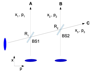
Figure 2: (Color online) Schematic of the generation of a genuinely tripartite entangled state, the CV GHZ state, using three squeezed input states. Here, BS1 and BS2 symbolize beam splitters, with reflectivities given by $R_{1}$ and $R_{2}$. For the GHZ state, $R_{1}=\frac{1}{3}$ and $R_{2}=\frac{1}{2}$. The $x_{j}$, $p_{j}$ refer to the two orthogonal quadrature phase amplitudes of the optical mode $j$ ($j=1,2,3)$, with boson operators $a_{j}$, $a_{j}^{\dagger}$. Three distinct modes are formed at the three outputs, $A$, $B$, and $C$. The $x-p$ axis and ellipses depict the orientation of the squeezing required.

The CV GHZ state braunghz is generated using the configuration shown in Fig. 2 cvsig . Two orthogonally squeezed vacuum modes are the inputs of a beam splitter (BS1). This creates a pair of entangled modes at the outputs of the first beam splitter BS1. The entanglement is like that first discussed by EPR in their argument for the completion of quantum mechanics, where the positions and momenta (quadrature phase amplitudes) are both perfectly correlated mdrepr ; epr . One of the entangled outputs is then combined across a second beam splitter (BS2) using a third squeezed state input. The squeeze parameters of the input states are assumed equal, and of magnitude given by $r$. This means that in the idealised experiment, each squeezed vacuum input has a quadrature variance given by $\Delta x=e^{\mp r}$ and $\Delta p=e^{\pm r}$ (the sign depending on the orientation of the squeezing and here we denote the ideal case of pure squeezed inputs). More generally, the two entangled modes could be created from parametric interactions mdrepr ; heid two mode above threshold ; twomodesq or similar atomic processes atomic tmss with dan . Tripartite entanglement can also be generated via three-photon parametric interactions involving pump fields, as in the studies of Villar et al.. claude .

A tripartite CV GHZ state is a simultaneous eigenstate of the position difference $x_{i}-x_{j}$ ($i,j=1,2$, or $3$, $i\neq j$) and the momentum sum $p_{1}+p_{2}+p_{3}$, and is formed in the limit of large $r$. The experiment of Aoki et al. aokicv used this generation process to give an approximate realization of the CV GHZ state, to the extent that they were able to demonstrate the full tripartite inseparability of the three modes (using the van Loock-Furusawa inequalities of Eq. (LABEL:eq:threeineq)).

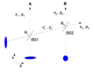
Figure 3: (Color online) Schematic of the generation of a genuinely tripartite entangled CV EPR-type state, using two squeezed input states and a vacuum input at the second beam splitter. Here, BS1 and BS2 are beam splitters, with reflectivities $R_{1}=R_{2}=0.5$. Labels as for Fig. 2.

In order to generate the second type of multipartite entangled state (which we call the CV EPR-type state) the third squeezed input is removed and replaced by a simple coherent vacuum state (Figure 3). The multipartite entanglement of these sorts of states has been investigated in the experiments of Armstrong et al. seiji ; seiji2 . These authors used the scheme of Figure 3 and its $N$-party extensions to generate states with a full $N$-partite inseparability, up to $N=8$ modes. The van Loock-Furusawa inequality approach was used to establish the inseparability.

The experimental confirmation of full $N$-partite inseparability does not establish genuine $N$-partite entanglement, unless one can justify pure states. In practice, this is not possible, because of losses and the difficulty in achieving pure input squeezed states. For this reason, we derive (in the following sections) criteria for genuine $N$- partite entanglement, and then examine the effectiveness of each criterion for the given CV states. We need to do this because the criteria are sufficient, but not necessary, to detect genuine multipartite entanglement. Calculations are therefore required to determine which criterion should be used for a given CV state. We will calculate the predictions for the criteria (which require moments of the $x_{k}$ and $p_{k}$), using the simple unitary transformation

$$a_{out,1} = \sqrt{R}a_{in,1}+\sqrt{1-R}a_{in,2}$$

$$a_{out,2} = \sqrt{1-R}a_{in,1}-\sqrt{R}a_{in,2}$$ (7)

that models the interaction of the modes at a beam splitter with reflectivity $R$. Here, $a_{out,1}$, $a_{out,2}$ are the two output modes and $a_{in,1}$, $a_{in,2}$ are the two input modes of the beam splitter.

IV Criteria for Genuine $N$-partite entanglement: general approach

We now explain a general method, that can be applied to detect the $N$-partite entanglement. For a given $N$, the complete set of bipartitions can be established. Let us suppose there are $X_{N}$ such bipartitions. We index the bipartitions by $k=1,..,X_{N}$, and denote by $A_{k}$ and $B_{k}$ the two distinct sets of parties defined by the bipartition $k$. For each bipartition $A_{k}-B_{k}$, we can establish an inequality $I_{k}\geq 4$ based on the assumption of separability of the system density operator $\rho$ with respect to that bipartition, where the $I_{k}$ is a sum $(\Delta u)^{2}+(\Delta v)^{2}$ of variances of linear combinations $u$, $v$ of system observables $x_{j}$ and $p_{j}$. This means that the observation of $I_{k}<4$ will imply failure of separability (entanglement) between $A_{k}$ and $B_{k}$. We can also establish similar inequalities $\mathcal{I}_{k}\geq 2$ where $\mathcal{I}_{k}$ is a product $\Delta u\Delta v$.

We note that there will be many such inequalities for a given bipartition, and that while $I_{k}<4$ suffices to imply inseparability between $A_{k}$ and $B_{k}$, it is not necessary, so that the choice of inequality is often intuitive, being dependent on the nature of the quantum state. The van Loock-Furusawa inequalities are an example of a set of inequalities $I_{k}$.

The violation of each of the inequalities $I_{k}\geq 4$ ($k=1,...,X_{N})$ will not in itself imply genuine $N$-partite entanglement. However, as might be expected, we can show that a large enough violation of all the inequalities will in the end be sufficient. Thus, we establish the following Result.

Result (1): Violation of the inequality

$$\sum_{k=1}^{X_{N}}I_{k}\geq 4$$ (8)

(or the inequality $\sum_{k=1}^{X_{N}}\mathcal{I}_{k}\geq 2$ involving the products) is sufficient to imply $N$-partite genuine entanglement.

Proof: We consider the $X_{N}$ bipartitions of the $N$-partite system. We wish to negate the possibility that the system is described by a mixture

$$\rho_{BS}=\sum_{k=1}^{X_{N}}P_{k}\rho_{A_{k},B_{k}}$$ (9)

where $P_{k}$ is a probability the system is separable across the bipartition $k$ (thus, $\sum_{k}P_{k}=1$). Separability across the bipartition $k$ means that the density matrix is of the form $\rho_{A_{k},B_{k}}=\sum_{R}\eta_{R}^{(k)}\rho_{A_{k}}\rho_{B_{k}}$, where here $\rho_{A_{k}}$ and $\rho_{B_{k}}$ are density matrices for subsystems $A_{k}$ and $B_{k}$ respectively. Consider a mixture of states as given by a density operator $\rho=\sum_{R}P_{R}\rho_{R}$, where $\sum_{R}P_{R}=1$ and $\rho_{R}$ is the density operator for a component state. For any such mixture, the variance $(\Delta X)^{2}$ of an observable $X$ cannot be less than the weighted sum of the variances of the component states: that is,

$$(\Delta X)^{2}\geq\sum_{R}P_{R}(\Delta_{R}X)^{2}$$ (10)

where $(\Delta_{R}X)^{2}$ denotes the variance of $X$ for the system in the state $\rho_{R}$ hoftake . Here, the observable $X$ is $u$ or $v$ as defined by Eqs. (3) and (4). For two such observables, we have the result

$$(\Delta X)^{2}+(\Delta Y)^{2}\geq\sum_{R}P_{R}\{(\Delta_{R}X)^{2}+(\Delta_{R}Y)^{2}\}$$ (11)

We can also prove a similar result for products of variances. In that case, applying the Cauchy-Scwharz inequality, we can see that

$$(\Delta X)(\Delta Y) \geq \{\{\sum_{R}P_{R}(\Delta_{R}X)^{2}\}\{\sum_{R}P_{R}(\Delta_{R}Y)^{2}\}\}^{1/2}$$ (12)

$$\geq \sum_{R}P_{R}(\Delta_{R}X)(\Delta_{R}Y)$$

Now, $I_{k}$ is the sum of variances. For example, $I_{k}=(\Delta u)^{2}+(\Delta v)^{2}$ can be the van Loock-Furusawa inequalities Eq. (LABEL:eq:threeineq) for certain values of linear coefficients. Similarly, $\mathcal{I}_{k}=\Delta u\Delta v$ and can be the product inequalities Eq. (LABEL:eq:threeineq-1). If the system is biseparable according to $\rho_{BS}$ of Eq. (1), then applying Eq. (11) it follows that

$$I_{k}\geq\sum_{m=1}^{X_{N}}P_{m}I_{k,m}\geq 4P_{k}$$

where $I_{k,m}$ is the value of the sum of the variances that form the expression $I_{k}$ evaluated over the biseparable state $\rho_{A_{m},B_{m}}$. We have used that for the separable state $\rho_{A_{k},B_{k}}$, $I_{k}\geq 4$. Summing over all $k$ and using that $\sum_{k=1}^{X_{N}}P_{k}=1$, we obtain $\sum_{k}I_{k}\geq 4$. Similarly, we can use Eq. (12) to prove $\mathcal{I}_{k}\geq\sum_{m=1}^{X_{N}}P_{m}\mathcal{I}_{k,m}\geq 2P_{k}$ and then that $\sum_{k}\mathcal{I}_{k}\geq 2$. $\square$

Where there is a redundancy so that one of the inequalities $I_{k}\geq 4$ is implied by more than one bipartition, we may be able to prove a stronger criterion. Certainly, if a single inequality $I\geq 4$ (or $\mathcal{I}\geq 2$) can negate separability with respect to all bipartitions $A_{k}-B_{k}$, then we can derive the following.

Result (2): Violation of the inequality

$$I\geq 4$$ (13)

(or $\mathcal{I}\geq 2$) which negates all of the biseparable states $\rho_{A_{k},B_{k}}$ ($k=1,...,X_{N})$ is sufficient to imply $N$-partite genuine entanglement.

Proof: Consider a system described by the biseparable mixture $\rho_{BS}$ of Eq. (9). Then using the results Eqs. (10) and (12) proved for mixtures, it follows that for such a system

$$I\geq\sum_{m=1}^{X_{N}}P_{m}I_{k,m}\geq 4$$

where we have used the result that $I\geq 4$ for every bipartition, i.e. for every biseparable state $\rho_{A_{k},B_{k}}$ and hence that each $I_{k.m}\geq 4$. Similarly, $\mathcal{I}\geq 2$.

The approach of using a single inequality is very valuable, once the inequality can be identified. We will show how to use this method for the CV GHZ and EPR-type states. Other criteria can be derived where there are intermediate redundancies, as for the three van Loock-Furusawa inequalities Eq. (LABEL:eq:threeineq). In that case, each inequality will negate separability with respect to two bipartitions. We obtain the following result.

Criterion (1): We confirm genuine tripartite entanglement, if the following inequality is violated:

$$B_{I}+B_{II}+B_{III}\geq 8$$ (14)

where $B_{I}\geq 4$ , $B_{II}\geq 4$ and $B_{III}\geq 4$ are the van Loock-Furusawa inequalities, Eq. (LABEL:eq:threeineq). We note that $B_{I}$, $B_{II}$, $B_{III}$ is a function of the variable parameters $g_{3}$, $g_{1}$, $g_{2}$ respectively.

Proof: For $N=3$ parties, there are three biseparable states $\rho_{23,1}$, $\rho_{13,2}$, and $\rho_{12,3}$ that we index by $k=1,2,3$ respectively. Consider any mixture of the form Eq. (1), which is Eq. (9) for $N=3$. Using the result Eq. (10) and the notation defined in the proof of Result (1), since $B_{I}$ is the sum of two variances, we can write

$$B_{I} \geq P_{1}B_{I,1}+P_{2}B_{I,2}+P_{3}B_{I,3}$$

$$\geq P_{1}B_{I,1}+P_{2}B_{I,2}\geq 4(P_{1}+P_{2})$$

This uses that we know the first two states of the mixture (for which $k=1,2$) will satisfy the inequality, $B_{I}\geq 4$. Hence, for any mixture $B_{I}\geq 4(P_{1}+P_{2})$. Similarly, $B_{II}\geq 4(P_{2}+P_{3})$ and $B_{III}\geq 4(P_{1}+P_{3})$. Then we see that since $\sum_{k=1}^{3}P_{k}=1$, for any mixture it must be true that $B_{I}+B_{II}+B_{III}\geq 8$. $\square$

The product version of the criterion follows along similar lines. The proof is similar to that of Criterion (1) and is given in the Appendix.

Criterion (2): We confirm genuine tripartite entanglement if the following inequality is violated:

$$S_{I}+S_{II}+S_{III}\geq 4$$ (15)

where $S_{I}\geq 2$ , $S_{II}\geq 2$ and $S_{III}\geq 2$ are the product van Loock-Furusawa-type inequalities, Eq. (LABEL:eq:threeineq-1).

V Criteria for Genuine tripartite entanglement

We now derive specific criteria to detect the genuine tripartite entanglement of the tripartite entangled CV GHZ and EPR-type states.

V.1 Criteria that use a single inequality

First we examine the case where the criterion takes the form of a single inequality involving just two variances, rather than the sum of three inequalities, as in Eqs. (14) and (15). Such criteria can be useful, but need to be tailored to the type of tripartite entangled state. In this Section, we present several such inequalities.

Criterion (3): The violation of the inequality

$$[\Delta(x_{1}-\frac{(x_{2}+x_{3})}{\sqrt{2}})]^{2}+[\Delta(p_{1}+\frac{(p_{2}+p_{3})}{\sqrt{2}})]^{2}\geq 2$$ (16)

is sufficient to confirm genuine tripartite entanglement.

Proof: Van Loock and Furusawa showed that the inequality is satisfied by all three biseparable states of types $\rho_{12,3}$, $\rho_{13,2}$, and $\rho_{23,1}$ cvsig . Hence, the proof follows on using the Result (2), given by Eq. (13). $\square$

Van Loock and Furusawa pointed out that this single inequality can be used to negate all three separable bipartitions $12-3$, $13-2$, and $23-1$, and hence to certify full tripartite inseparability. However, the application of the Eq. (10) for mixtures is needed to complete the proof that this single inequality is indeed sufficient to certify genuine tripartite entanglement. Before continuing, we write the product version of this criterion.

Criterion (4): The violation of the inequality

$$\Delta(x_{1}-\frac{(x_{2}+x_{3})}{\sqrt{2}})\times\Delta(p_{1}+\frac{(p_{2}+p_{3})}{\sqrt{2}})\geq 1$$ (17)

is sufficient to confirm genuine tripartite entanglement.

Proof: The uncertainty relation $\Delta x_{j}\Delta p_{j}\geq 1$ implies that the inequality $\Delta u\Delta v\geq 1$ holds for all three types of states $\rho_{12,3}$, $\rho_{13,2}$, and $\rho_{23,1}$. This follows directly from the result Eq. (4). $\square$

We see immediately that violation of Eq. (16) will always imply violation of Eq. (17). (Since $x^{2}+y^{2}\geq 2xy$ for any two real numbers $x$, $y$). Thus, the product criterion (4) is a stronger (better) criterion. However, where $\Delta(x_{1}-\frac{(x_{2}+x_{3})}{\sqrt{2}})=\Delta(p_{1}+\frac{(p_{2}+p_{3})}{\sqrt{2}})$, the two criteria are mathematically equivalent. (We note $x^{2}+y^{2}=2xy$ iff $x=y$). This is the case for the states we consider in this paper, but is not true in general. For some other states, entanglement criteria based on products of variances have proved useful product ; prod2 .

The two simple criteria (16) and (17) are effective for demonstrating the genuine tripartite entanglement of the EPR-type state, as shown by in the recent paper of Armstrong et al. seiji2 where the product criterion (16) was derived. The predictions are plotted in Figure 4.

For the CV GHZ state, it is better to consider a more generalised criterion that allows arbitrary coefficients.

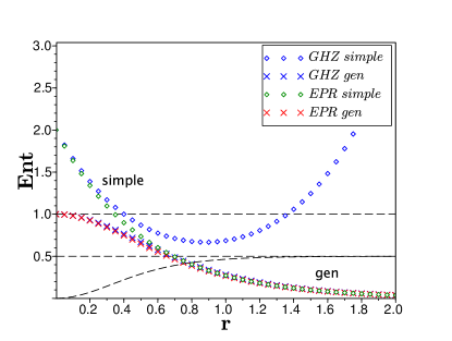
Figure 4: (Color online) Detecting the genuine tripartite entanglement of the CV GHZ and EPR-type states of Figures 2 and 3: $Ent<1$ signifies genuine tripartite entanglement. Here, $r$ is the squeezing parameter of the input states shown in Figs. 2and3. The curves labeled “simple” are for the (top blue) GHZ and (second green) EPR-type states, using the simple criteria (16) and (17) (which give indistinguishable results). The two lower curves labeled “gen” are for the GHZ and EPR-type states, using the generalized criteria (18) and (20) (which give indistinguishable results). Here, $Ent=\frac{(\Delta u)^{2}+(\Delta v)^{2}}{2}$ and $Ent=\Delta u\Delta v$ for the criteria involving sums and products respectively, where $u=x_{1}+h(x_{2}+x_{3})$, $v=p_{1}+g(p_{2}+p_{3})$. The choices for $h$ and $g$ are given in Table 1 for the generalized criteria, and are $g=-h=\frac{1}{\sqrt{2}}$ for the simple criteria. Genuine tripartite steering is signified when $Ent$ drops below the black dashed line for the “gen” case, and below $0.5$ for the “simple” curves. All curves except the “simple GHZ” become indistinguishable at larger $r$.

Criterion (5): Violation of the inequality

$$(\Delta u)^{2}+(\Delta v)^{2} \geq 2\min{\{|g_{3}h_{3}|+|h_{1}g_{1}+h_{2}g_{2}|,}$$ (18)

$$|g_{2}h_{2}|+|h_{1}g_{1}+h_{3}g_{3}|,$$

$$|g_{1}h_{1}|+|g_{2}h_{2}+h_{3}g_{3}|\}$$

where we define $u=h_{1}x_{1}+h_{2}x_{2}+h_{3}x_{3}$ and $v=g_{1}p_{1}+g_{2}p_{2}+g_{3}p_{3}$ is sufficient to confirm genuine triparite entanglement. Here, $g_{i}$, $h_{i}$ are real constants ($i=1,2,3$).

Proof: Using Eq. (3), we see that the bipartition $\rho_{12}\rho_{3}$ implies

$$(\Delta u)^{2}+(\Delta v)^{2}\geq 2\{|g_{3}h_{3}|+|h_{1}g_{1}+h_{2}g_{2}|\},$$

the bipartition $\rho_{13}\rho_{2}$ implies

$$(\Delta u)^{2}+(\Delta v)^{2}\geq 2\{|g_{2}h_{2}|+|h_{1}g_{1}+h_{3}g_{3}|\},$$

and the bipartition $\rho_{23}\rho_{1}$ implies

$$(\Delta u)^{2}+(\Delta v)^{2}\geq 2\{|g_{1}h_{1}|+|g_{2}h_{2}+h_{3}g_{3}|\}.$$

Thus, using the relation Eq. (10), we see that any mixture Eq. (1) will imply Eq. (18). $\square$

Table 1: Values of $g$ and $h$ used for the plots of Fig 4.

r	CV GHZ		EPR
	g	h	g	h
0	0	0	0	0
0.25	0.36	-0.27	0.33	-0.33
0.5	0.68	-0.40	0.54	-0.54
0.75	0.86	-0.46	0.64	-0.64
1	0.95	-0.49	0.68	-0.68
1.5	0.99	-0.50	0.70	-0.70
2	1.00	-0.50	0.70	-0.70

The Criterion (5) is valid for any choice of coefficients $g_{i}$ and $h_{i}$, which are real constants. If the inequality is violated, then the experimentalist can conclude the three modes are genuine tripartite entangled. However, as the criteria are sufficient but not necessary for entanglement, it cannot be assumed that the inequality will be violated, even where there is entanglement present. In a practical situation for a given entangled state, it is best to analyze in advance the optimal values for $g$, $h$. These optimal values are defined as giving the smallest ratio of the left to right side of the inequality, for a given quantum state.

An optimization was carried out numerically, for a simpler version of the inequalities obtained as follows: A simpler version of the inequality (18) is obtained, if we select the values $g_{1}=h_{1}=1$, $h_{2}=h_{3}=h$, and $g_{2}=g_{3}=g$ so that $u=x_{1}+h(x_{2}+x_{3})$ and $v=p_{1}+g(p_{2}+p_{3})$, and then restrict to $gh<0$ and $|gh|<1$. We note that the right side of Eq. (18) becomes $2\min\{|gh|+|1-|gh||,1+2|gh|\}$. Eq. (18) then takes the form

$$(\Delta u)^{2}+(\Delta v)^{2}\geq 2.$$ (19)

Violation of this inequality will confirm genuine tripartite entanglement (as a special case of Criterion (5)). The theoretical prediction for the optimal value of gain constants $g$ and $h$ was found rigorously by a numerical search over all values. The optimized values and associated violation of the inequalities for the CV GHZ and EPR-type states are given in Table I and Fig. 4.

An experimental set-up to detect the genuine tripartite entanglement is like that described in Ref. cvsig and implemented in the experiment aokicv , to detect full tripartite inseparability. Ideally, in a tripartite version of an EPR experiment, the quadrature amplitudes would be measured simultaneously in a spacelike separated way at each of the three locations epr ; rmp-1 . The inequalities are tested by direct insertion of the results into the inequality, with the $g$ and $h$ serving as numbers. In the experiments modeled after squeezing measurements aokicv ; mdrepr ; ou epr-1 , the final variances are measured directly as noise levels, and the $g$ and $h$ factors are introduced by classical gains in currents.

We also derive the product form of the generalized criterion (18). The proof is similar to that for Criterion Eq. (18) and is given in the Appendix.

Criterion (6): Genuine tripartite entanglement is observed if the inequality

$$\Delta u\Delta v \geq \min{\{|g_{3}h_{3}|+|h_{1}g_{1}+h_{2}g_{2}|,}$$ (20)

$$\{|g_{2}h_{2}|+|h_{1}g_{1}+h_{3}g_{3}|,$$

$$|g_{1}h_{1}|+|g_{2}h_{2}+h_{3}g_{3}|\}$$

is violated. With the choice of values for $g_{i}$ and $h_{i}$ explained for the inequality (19) and as given in Table 1, the inequality (20) takes the simpler form

$$\Delta u\Delta v\geq 1.$$ (21)

While the optimal values of the coefficients $g$ and $h$ were found by numerical search, it is possible to deduce these values from the physics associated with the different entangled states, at least in the limit of large $r$. We see from the results of Table 1 and Figure 4 that for larger $r$, the genuine tripartite entanglement of the CV GHZ state is detected by violation of the inequality

$$[\Delta(x_{1}-\frac{(x_{2}+x_{3})}{2})]^{2}+[\Delta(p_{1}+p_{2}+p_{3})]^{2}\geq 2$$ (22)

This is to be expected, since the CV GHZ state formed in the limit of large $r$ is by definition the simultaneous eigenstate of position difference $x_{i}-x_{j}$ ($i,j=1,2$ or $3$, $i\neq j$) and the momentum sum $p_{1}+p_{2}+p_{3}$.

Similarly, for the EPR-type states of Fig. 3, the simple Criterion of Eq. (16) (and Eq. (17)) is in fact optimal at large $r$. This can be understood as follows cvsig : The two entangled modes labeled $1$ and $2^{\prime}$ in Fig. 3 possess an EPR correlation as $r\rightarrow\infty$, so that simultaneously, both $[\Delta(x_{1}-x^{\prime}_{2})]^{2}\rightarrow 0$ and $[\Delta(p_{1}+p^{\prime}_{2})]^{2}\rightarrow 0$ where $x^{\prime}_{2}$ and $p^{\prime}_{2}$ are the quadratures of the mode defined as $2^{\prime}$. On examining the model of Eq. (7) for the beam splitter interaction $BS2$, we put $a_{out,1/2}=a_{2/3}$, $a_{in,1}=a_{2^{\prime}}$ and $a_{in,2}=a_{vac}$ where $a_{vac}$ is the boson operator for the vacuum mode input to $BS2$. Then we see that for $R=0.5$, $a_{2^{\prime}}=\frac{1}{\sqrt{2}}(a_{2}+a_{3})$, which leads to the solution $x^{\prime}_{2}=\frac{1}{\sqrt{2}}(x_{2}+x_{3})$ and $p^{\prime}_{2}=\frac{1}{\sqrt{2}}(p_{2}+p_{3})$. Thus, the EPR correlation of the original beams $1$ and $2^{\prime}$ is transformed into a tripartite EPR correlation that satisfies the Criterion (3) of Eq. (16). This is the reason why we call these states “EPR-type”. We note that as the EPR (or GHZ) correlation increases (as it does with large $r$), the associated variances reduce, so the amount of violation of the inequalities gives an indication of the strength of that type of EPR (GHZ) entanglement.

We point out that the noise reduction required to demonstrate the genuine tripartite entanglement is considerable, in the sense of being beyond that necessary to demonstrate simple quantum squeezing, or bipartite entanglement. Let us consider the group of modes $\{2,3\}$ created at the output of the second beam splitter $BS2$ as shown in Figure 3. Bipartite entanglement between mode $1$ and the combined group of modes $\{2,3\}$ can be certified when $(\Delta u)^{2}+(\Delta v)^{2}<4$, which corresponds to a noise reduction below the noise level of the quantum vacuum (measured by $4$ in this case). The bipartite entanglement condition can be verified using the techniques of Refs. duan-1 ; product . Thus, the Criterion (3) of Eq. (16) to confirm genuine tripartite entanglement requires 50% greater violation than to confirm ordinary bipartite entanglement.

V.2 Criteria using van Loock-Furusawa inequalities

Violation of the van Loock-Furusawa inequalities (Eq. (5)) have been measured or calculated in numerous situations (including claude ; aokicv ; murraytri ; seiji ). In Figure 5, we use the Criteria (1) and (2), as given by Eqs. (14 and 15), to show that it is possible to verify the genuine tripartite entanglement using the van Loock-Furusawa inequalities, provided there is enough violation of the inequalities.

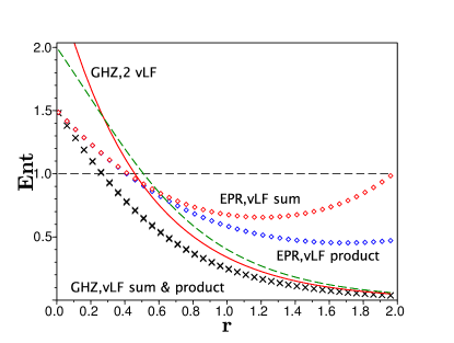
Figure 5: (Color online) Detecting genuine $N$-partite entanglement by summation of the violation of van Loock-Furusawa (vLF) inequalities, or their product versions. $Ent<1$ signifies genuine tripartite entanglement; $Ent<0.5$ signifies genuine tripartite steering. The description of states and the meaning of $r$ is as in Figure 4. For the Criterion (4) given by Eq. (15), $Ent=(S_{I}+S_{II}+S_{III})/4$ (product version) and for the Criterion (3) given by Eq. (14), $Ent=(B_{I}+B_{II}+B_{III})/8$ (sum version). The choice of $g_{i}$’s is given in Table 2. The black (lower) crosses and blue (lower) diamonds give results for the product criterion, for GHZ and EPR-type states, respectively, with $N=3$. The Criteria (3) and (4) give indistinguishable results for the GHZ state. The upper red diamond curve is the Criterion (3) for the $N=3$ EPR-type state. The red line gives Criterion (7) (Eq. (23)), involving just two vLF inequalities, for the GHZ state, where $Ent=(B_{I}+B_{II})/4$. The green dashed line is the Criterion (9) (Eq. (43)) for the GHZ state ($N=4$).

For symmetric systems such as the CV GHZ state, where $B_{I}=B_{II}=B_{III}$, the condition (LABEL:eq:threeineq-1) of Criterion (1) requires $B_{I}<8/3$. This level of noise reduction (which is $2/3$ the vacuum noise level) would seem feasible in the set-up of experiment aokicv . The ideal CV GHZ state clearly violates the inequality, since in that case $B_{I}=B_{II}=B_{III}\rightarrow 0$ as $r\rightarrow\infty$. The inequality for $g_{i}=1$ has been derived by Shalm et al.. shalm-1 . We note from Table 2 that for the GHZ state the values of $g_{1}=g_{2}=g_{3}=1$ are indeed optimal as $r\rightarrow\infty$. The criterion derived here is valid for arbitrary $g$’s, which we see from Table 2 is useful for the EPR-type states of Fig. 3. These EPR-type states do not have symmetry with respect to all three modes.

The effectiveness of the criteria is shown in the Figure 5 for the CV GHZ and EPR-type states. It is not surprising that the criteria are more effective in the case of the GHZ states. This is because the van Loock-Furusawa inequalities include terms involving the variance of $x_{k}-x_{m}$ ($k\neq m$) which for the GHZ state (but not the EPR-type state) will be small as $r\rightarrow\infty$.

Table 2: Values of $g_{i}$ ($i=1,2,3$) for the plots of Figure 5. The same values are used for the sum and product versions of the criteria.

r	$g_{1}$	GHZ $g_{2}$	$g_{3}$	$g_{1}$	EPR $g_{2}$	$g_{3}$
0	0	0	0	0	0	0
0.25	0.53	0.53	0.53	0.63	0.29	0.29
0.5	0.81	0.81	0.81	1.08	0.44	0.44
0.75	0.93	0.93	0.93	1.28	0.50	0.50
1	0.97	0.97	0.97	1.36	0.50	0.50
1.5	1.00	1.00	1.00	1.41	0.46	0.46
2	1.00	1.00	1.00	1.41	0.43	0.43

V.3 Criteria involving just two van Loock-Furusawa inequalities

The following criterion involving just two inequalities but with $g_{i}=1$ has been derived by Shalm et al. shalm-1 .

Criterion (7): We can confirm genuine tripartite entanglement, if any two of the inequalities $B_{I}\geq 4$, $B_{II}\geq 4$, $B_{III}\geq 4$ given by Eq. (LABEL:eq:threeineq) with $g_{1}=g_{2}=g_{3}=1$ are violated by a sufficient margin, so that

$$B_{I}+B_{II}<4$$ (23)

(or $B_{I}+B_{III}<4$, or $B_{II}+B_{III}<4$).

The symmetry of the GHZ state means that the genuine tripartite entanglement is detected using any one of these the inequalities. Where losses are important, this can change. These criteria are not effective in detecting the genuine tripartite entanglement of the EPR-type states, for the reasons discussed above, that the variances of the van Loock-Furusawa inequalities do not capture the correlated observables in this case.

VI Criteria for genuine tripartite EPR steering

We now consider criteria to detect the type of entanglement called “genuine tripartite EPR steering”. EPR steering is a nonlocality associated with the EPR paradox, that can be regarded in some sense intermediate between entanglement and Bell’s nonlocality hw-1 ; bell . We follow and expand on the methods of Ref. genepr . The criteria are the same inequalities as before, but with stricter bounds. The physical significance of EPR steering is that it allows detection of the entanglement even when some of the parties or measurement devices associated with the systems $i=1,2,3$ cannot be trusted cv trust ; one-sidedcrytpt . For example, we may not be able to assume that the results reported by some parties are actually the result of quantum measurements $\hat{x}$ or $\hat{p}$. This can be important where the entanglement is used for quantum key distribution one-sidedcrytpt .

Consider three measurements $X_{1}$, $X_{2}$ and $X_{3}$ made on each of three distinct systems (also referred to as parties). Where the composite system is given by the biseparable density matrix $\rho_{BS}$ of Eq. (1), we note that any average $\langle X_{1}X_{2}X_{3}\rangle$ is expressible as

$$\langle X_{1}X_{2}X_{3}\rangle = P_{1}\sum_{R}\eta_{R}^{(1)}\langle X_{2}X_{3}\rangle_{R}\langle X_{1}\rangle_{R,\rho}$$ (24)

$$+P_{2}\sum_{R}\eta_{R}^{(2)}\langle X_{1}X_{3}\rangle_{R}\langle X_{2}\rangle_{R,\rho}$$

$$+P_{3}\sum_{R}\eta_{R}^{(3)}\langle X_{1}X_{2}\rangle_{R}\langle X_{3}\rangle_{R,\rho}$$

Here all averages $\langle\rangle$ are those of a quantum density matrix, and the $\rho$ subscript reminds us of that. To signify genuine tripartite Bell nonlocality bell , however, one needs to falsify a stronger assumption. This can be done, if we falsify (24), but without the assumption that the averages $\langle\rangle$ are necessarily those of quantum states: They can be averages for hidden variable states, as defined by Bell and Svetlichny svetlichny ; gallego .

To signify genuine tripartite steering genepr , it is sufficient to falsify a hybrid local-nonlocal “biseparable Local Hidden State (LHS) model”, which is a multiparty extension of the bipartite LHS models defined in Refs. hw-1 ; ericmultisteer . In that case, the averages $\langle X_{k}X_{m}\rangle_{R}$ (that are without the subscript $\rho$) can be hidden variable averages, whereas those for the single system $\langle X_{n}\rangle_{R,\rho}$ (written with the subscript $\rho$) are quantum averages.

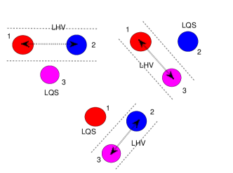
Figure 6: (Color online) Schematic of the hybrid Local-Nonlocal Hidden States that if negated signify genuine tripartite steering. The three depictions are hidden variable models, in which nonlocality is allowed between any two of the three systems (labeled $1,2,3$). The top left model is denoted $\{12,3\}_{st}$: Here, nonlocality and therefore steering (arrows) is allowed between systems $1,2$, which together form a local hidden variable state (LHV). There is no steering between systems $1,2$ and system $3$, which in the model is constrained to be a local quantum state (LQS). The other models are $\{13,2\}_{st}$ (top right) and $\{23,1\}_{st}$ (lower). Failure of all three models (and any probabilistic mixtures of them) will signify genuine tripartite steering.

We introduce a notation to explain this (Fig. 6). For $N=3$, there are three bipartitions of the systems: $23-1$, $13-2$, $12-3$. The biseparable LHS description given by Eq. (24) assumes bipartitions $km-n$, but where only the system $n$ need be a quantum system. We denote these special types of bipartition by the notation $\{23,1\}_{st}$, $\{13,2\}_{st}$, $\{12,3\}_{st}$. Specifically, negation of the bipartition $\{23,1\}_{st}$, implies that we cannot write the moment $\langle X_{3}X_{2}X_{1}\rangle$ in the form $\langle X_{3}X_{2}X_{1}\rangle=\sum_{R}\eta_{R}^{{}^{(1)}}\langle X_{3}X_{2}\rangle\langle X_{1}\rangle_{\rho}$. This negation implies that system $1$ is “steerable” by system $\{2,3\}$ hw-1 .

The key point to the derivations of the steering criteria is that we can only assume the quantum uncertainty relation for some of the systems. This has been explained in Ref. genepr . First, we assume the bipartition $\{km,n\}_{s}$ where only system $n$ is constrained to be a quantum state. Letting $u=h_{k}x_{k}+h_{m}x_{m}+h_{n}x_{n}$ and $v=g_{k}p_{k}+g_{m}p_{m}+g_{n}p_{n}$, it can then be shown that the two inequalities hold (see Appendix and Ref. genepr ):

$$(\Delta u)^{2}+(\Delta v)^{2} \geq 2|h_{n}g_{n}|.$$ (25)

$$\Delta u\Delta v \geq |h_{n}g_{n}|$$ (26)

These relations lead to criteria for genuine tripartite steering. In the following, we write the “EPR steering versions” of the Criteria (1-6). The proofs have been given in Ref. genepr or else are in the Appendix.

To understand the significance of this sort of steering, we note that the falsification of the biseparable state $\{km-n\}_{st}$ implies a steering of $n$ by $km$: this means entanglement can be proved between $n$ and the group $km$, without the assumption of good devices for systems $km$. This type of genuine tripartite steering falsifies any possible mixture of such bipartitions, and therefore certainly falsifies each one of them. Therefore, the genuine tripartite steering is certainly sufficient to imply that any two parties can “steer” the third. In demonstrating genuine tripartite steering, it is negated that the steering of the three-party system can be described by consideration of two-party steering models alone. This confirms a genuine sharing of steering among three systems, and gives insight into a fundamental property of quantum mechanics.

Criteria (3s), (4s): Genuine tripartite EPR steering is observed if

$$[\Delta(x_{1}-\frac{(x_{2}+x_{3})}{\sqrt{2}})]^{2}+[\Delta(p_{1}+\frac{(p_{2}+p_{3})}{\sqrt{2}})]^{2}\geq 1$$ (27)

is violated (Criterion (3s)), or if

$$\Delta(x_{1}-\frac{(x_{2}+x_{3})}{\sqrt{2}})\times\Delta(p_{1}+\frac{(p_{2}+p_{3})}{\sqrt{2}})\geq 0.5$$ (28)

is violated (Criterion (4s)). These steering inequalities are used in Figure 4. The proofs have been given in Refs. genepr and seiji2 , and are given in our notation in the Appendix.

Criteria (5s), (6s): The violation of either one of the inequalities

$$(\Delta u)^{2}+(\Delta v)^{2} \geq 2\min\{|g_{1}h_{1}|,|g_{2}h_{2}|,|g_{3}h_{3}|\},$$ (29)

$$\Delta u\Delta v \geq \min\{|g_{1}h_{1}|,|g_{2}h_{2}|,|g_{3}h_{3}|\},$$ (30)

where $u=h_{1}x_{1}+h_{2}x_{2}+h_{3}x_{3}$, $v=g_{1}p_{1}+g_{2}p_{2}+g_{3}p_{3}$ is sufficient to confirm genuine tripartite EPR steering.

Proof: Using Eq. (25), we see that the bipartition $\{12,3\}_{s}$ gives the constraint $(\Delta u)^{2}+(\Delta v)^{2}\geq 2|g_{3}h_{3}|$; the bipartition $\{13,2\}_{s}$ implies $(\Delta u)^{2}+(\Delta v)^{2}\geq 2|g_{2}h_{2}|$; and the bipartition $\{23,1\}_{s}$ implies $(\Delta u)^{2}+(\Delta v)^{2}\geq 2|g_{1}h_{1}|$. Thus, using Eq. (10), for any mixture of the bipartitions, we can say that

$$(\Delta u)^{2}+(\Delta v)^{2}\geq 2\min\{|g_{1}h_{1}|,|g_{2}h_{2}|,|g_{3}h_{3}|\}.$$ (31)

Violation of Eq. (31) confirms genuine tripartite steering. The product result follows similarly, from (26). $\square$

We can simplify these Criteria. On putting $g_{1}=h_{1}=1$ and selecting $h_{2}=h_{3}=h$ and $g_{2}=g_{3}=g$, the right side of the inequality becomes $2\min\{1,|gh|\}$. Now, if we take $|gh|<1$ as in Table 1, the inequalities take the simpler form

$$(\Delta u)^{2}+(\Delta v)^{2}\geq 2|gh|$$ (32)

and $\Delta u\Delta v\geq|gh|$. This inequality is used to demonstrate genuine tripartite EPR steering, in Fig. 4.

It is now possible to derive a set of three “EPR steering inequalities” similar to those derived by van Loock and Furusawa. This has been explained in Ref. genepr . The assumption that the system is in one of the bipartitions $\{km,n\}_{st}$ will lead to a “steering inequality”, that if violated implies system $n$ is steerable by the combined two systems $\{km\}$. Considering each of the three possible bipartitions, there are three “steering” inequalities identical to the van Loock and Furusawa inequalities cvsig but with a different right-side bound:

$$B_{I}\equiv[\Delta(x_{1}-x_{2})]^{2}+[\Delta(p_{1}+p_{2}+g_{3}p_{3})]^{2} \geq 2,$$

$$B_{II}\equiv[\Delta(x_{2}-x_{3})]^{2}+[\Delta(g_{1}p_{1}+p_{2}+p_{3})]^{2} \geq 2,$$

$$B_{III}\equiv[\Delta(x_{1}-x_{3})]^{2}+[\Delta(p_{1}+g_{2}p_{2}+p_{3})]^{2} \geq 2,$$

In fact, inequality $B_{I}\geq 2$ is implied by bipartitions $\{23,1\}_{s}$ and $\{13,2\}_{s}$; inequality $B_{II}\geq 2$ is implied by $\{13,2\}_{s}$ and $\{12,3\}_{s}$; and inequality $B_{III}\geq 2$ is implied by $\{12,3\}_{s}$ and $\{23,1\}_{s}$. Thus, $B_{I}<2$ signifies steering of 1 by $\{23\}$, and also steering of $2$ by $\{13\}$, etc. The proof of these inequalities is as for the original proof of the van Loock-Furusawa inequalities, but assuming only the uncertainty relation $\Delta x\Delta p\geq 1$ for the steered system $n$ genepr . A second associated set of EPR steering inequalities involving products can also be derived:

$$S_{I}\equiv\Delta(x_{1}-x_{2})\Delta(p_{1}+p_{2}+g_{3}p_{3}) \geq 1,$$

$$S_{II}\equiv\Delta(x_{2}-x_{3})\Delta(g_{1}p_{1}+p_{2}+p_{3}) \geq 1,$$

$$S_{III}\equiv\Delta(x_{1}-x_{3})\Delta(p_{1}+g_{2}p_{2}+p_{3}) \geq 1,$$

These are the steering versions of the product inequalities Eq. (LABEL:eq:threeineq-1). Here, inequality $S_{I}\geq 1$ is implied by bipartitions $\{23,1\}_{s}$ and $\{13,2\}_{s}$; inequality $S_{II}\geq 1$ is implied by $\{13,2\}_{s}$ and $\{12,3\}_{s}$; and inequality $S_{III}\geq 1$ is implied by $\{12,3\}_{s}$ and $\{23,1\}_{s}$. Thus, $S_{I}<2$ signifies steering of 1 by $\{23\}$, and also steering of $2$ by $\{13\}$, etc.

The inequalities lead us to the steering versions of the Criteria (1) and (2), used in Figure 5.

Criterion (1s), (2s): We confirm genuine tripartite steering if either the inequality

$$B_{I}+B_{II}+B_{III}\geq 4$$ (35)

or the inequality $S_{I}+S_{II}+S_{III}\geq 2$ is violated. Here, $B_{I}\geq 4$ , $B_{II}\geq 4$, and $B_{III}\geq 4$ are the van Loock-Furusawa inequalities, Eq. (LABEL:eq:threeineq) and $S_{I}\geq 2$ , $S_{II}\geq 2$, and $S_{III}\geq 2$ are the product van Loock-Furusawa-type inequalities, Eq. (LABEL:eq:threeineq-1). We note that each of $B_{I}$, $B_{II}$, $B_{III}$ is a function of the variable parameters $g_{1}$, $g_{2}$, $g_{3}$, respectively. The proof is given in the Supplemental Material of Ref. genepr , and is given in our own notation in the Appendix.

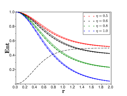
Figure 7: (Color online) The genuine tripartite entanglement of the CV GHZ and EPR-type states (Figures 2 and 3) with loss on the mode labeled $1$: The efficiency of the beam 1 is given by $\eta$. $Ent<1$ signifies genuine tripartite entanglement. We use the Criteria (5) and (6) with $h$ and $g$ given by Table 1. We signify genuine tripartite steering if $Ent$ is below the black dashed line, as given by Criteria (5s) and (6s). The efficiency of transmission for the beam $1$ is $\eta$. The $+$ curves are for the EPR-type state using the sum or product criterion, the two criteria giving indistinguishable results here. The second (upper) line of each pair of the same color gives the result for the GHZ state using the product criterion.

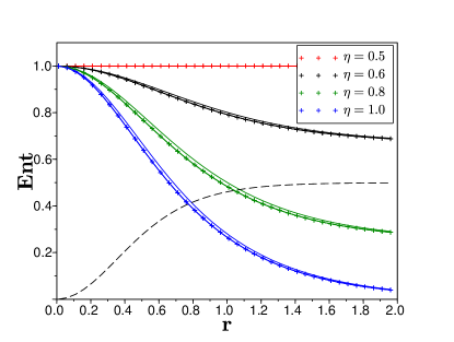
Figure 8: (Color online) The genuine tripartite entanglement of the CV GHZ and EPR-type states (Figs. 2 and 3) with loss on the modes labeled $2$ and $3$: $Ent<1$ signifies genuine tripartite entanglement. Labels and curves as for Figure 7. The efficiency of transmission for each of the beams 2 and 3 is given by $\eta$.

VII Effect of Losses

So far, we have only considered detection of genuine tripartite entanglement for pure states. However these idealized states are difficult to generate in the laboratory. There are two main sources of imperfection in the experiments: the impurity of the input squeezed states and the losses that occur during transmission along the channels. In this section, we analyze the effect of losses.

The transmission losses can be modeled using a simple beam-splitter model, in which the outputs after loss are given by $a_{out}=\sqrt{\eta}a_{in}+\sqrt{(1-\eta)}a_{vac}$, where $a_{in}$ is the mode before loss, $a_{vac}$ is a quantum vacuum mode, and $\eta$ is the efficiency factor that gives the altered transmission intensity of the field mode after the loss has taken place.

The effect of loss on the genuine tripartite entanglement as detected by the Criteria (5) and (6) is shown in Figs. 7 and 8. The most notable feature of the curves is the loss of the criterion as $\eta\rightarrow 0.5$. This can be explained based on a knowledge of steering. Generally, we say that a system $1$ is steerable by a group of systems labeled $B$ if we can show $[\Delta(x_{1}-x_{B})]^{2}+[\Delta(p_{1}+p_{B})]^{2}<2$ (or $\Delta(x_{1}-x_{B})\Delta(p_{1}+p_{B})<1$) rmp-1 ; hw-1 ; mdrepr . Here, $x_{B}$ and $p_{B}$ can be any measurements for system $B$. Then we note that as $r\rightarrow\infty$, the genuine tripartite entanglement criteria used in the Figures are given by violation of the inequalities Eqs. (16) and (22), which are precisely of the form that signifies steering of mode $1$ by the system $\{2,3\}$. It has also been shown based on monogamy relations that steering cannot take place with 50% or more loss on the steering system (in this case, {${2,3\}}$) monog . This explains the impossibility of the Criteria (5) and (6) being satisfied (for large $r$) in Figure 8 for $\eta\leq 0.5$.

We note that there is not the same restriction if we put the losses on the steered party monog , and hence the reduced sensitivity to losses shown in the plots of Figure 7, where the loss is entirely on party $1$. Also, we can manipulate the criteria $Ent<1$ given by the inequalities Eq. (16) and Eq. (22) into the form $[\Delta(x_{2}-x_{B})]^{2}+[\Delta(p_{2}+p_{B})]^{2}<4$ where now $B$ is the system containing modes $1$ and $3$. With $50\%$ loss on the modes $1$ and $3$, we cannot demonstrate the steering of mode $2$, which implies that $[\Delta(x_{2}-x_{B})]^{2}+[\Delta(p_{2}+p_{B})]^{2}>2$. Thus, we will observe $Ent>0.5$ in this case. This illustrates the asymmetry of the Criterion (5) with respect to the three parties. In short, this means that where transmission losses on a particular party (say $1$) are significant, it will be necessary to select the appropriate entanglement criterion.

VIII Criteria for Genuine $N$-partite entanglement

The above approaches can be generalized to higher $N$. Genuine $N$-partite entangled states can be generated by extending the schemes of Fig. 2, as explained in Refs. cvsig ; seiji and depicted in Figs. 9-11 for $N=4$. To prove genuine $N$-partite entanglement, one needs to negate all mixtures of the biseparable states, as explained in Sec. II. In this section, we consider three types of multipartite entangled states, as depicted for $N=4$ in Figs. 9-11. The first are the CV GHZ states, studied in Refs. cvsig ; braunghz ; aokicv , and generated by successively applying beam splitters to one of the entangled modes, with specified squeezed inputs. The second are the asymmetric EPR-type states I, studied in Ref. cvsig and formed by a sequence of beam splitters applied to one of the original two entangled modes. These states are depicted in Figure 10 for $N=4$. The third are the alternative EPR-type states, that we call symmetric EPR-type states II, formed by applying successive beam splitters to both arms of the entangled pair (Figure 11). These have been generated in Ref. seiji .

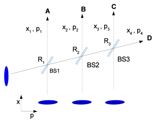
Figure 9: (Color online) Schematic of the generation of a genuinely four-partite entangled state: the CV GHZ state, formed using squeezed inputs where $R_{1}=\frac{1}{4}$, $R_{2}=\frac{1}{3}$, and $R_{3}=\frac{1}{2}$. The generalization to arbitrary $N$ is discussed in the Ref. cvsig .

VIII.1 Criteria for $N$-partite entanglement that use a single inequality

First, we extend the method described in the earlier sections, and look for a single inequality (involving just two variances) that may be effective as criterion for detecting the genuine $N$- partite entanglement. As we learned from the previous sections, we expect the best choice of inequality will be related to how the entangled state is generated.

Van Loock and Furusawa cvsig considered the following inequality for $u=x_{1}-\frac{1}{\sqrt{N-1}}(\sum_{i=2}^{N}x_{i})$ and $v=p_{1}+\frac{1}{\sqrt{N-1}}(\sum_{i=2}^{N}p_{i})$. They showed that

$$(\Delta u)^{2}+(\Delta v)^{2}\geq\frac{4}{(N-1)}$$ (36)

is satisfied by all biseparable states in the $N$ mode case. Hence, using Result (2) given by Eq. (13), we deduce that violation of this inequality will be sufficient to signify genuine $N$-partite entanglement. This will be useful to detect the $N$-partite entanglement of the asymmetric EPR-type state I, depicted for $N=4$ in Figure 10.

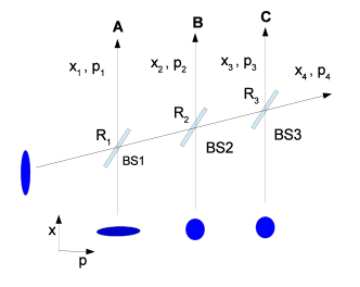
Figure 10: (Color online) Schematic of the generation of a genuinely four-partite entangled state: the asymmetric EPR-type state $I$ formed using a vacuum input at all but the first beam splitter and with $R_{1}=\frac{1}{2},R_{2}=\frac{1}{3},R_{3}=\frac{1}{2}.$ By applying a further sequence of beam splitters $R_{1}=\frac{1}{2},R_{2}=\frac{1}{N-1},R_{3}=\frac{1}{(N-1)-1}...,R_{N-1}=\frac{1}{(N-1)-(N-3)}$, as explained in the Ref. cvsig , this state can be generalized to arbitrary $N$.

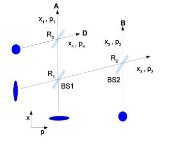
Figure 11: (Color online) Schematic of the generation of a genuinely four-partite entangled state: the symmetric EPR-type state $II$ created when $R_{1}=\frac{1}{2}$, $R_{2}=\frac{1}{2}$ and $R_{3}=\frac{1}{2}$. The generalization to arbitrary $N$ is discussed in the Ref. seiji

Here, we generalize the inequality (36), deriving a criterion that is also useful to detect the multipartite entanglement of the second type of EPR-type state II for $N=4$.

Criterion (8): We define $u=\sum_{i}h_{i}x_{i}$ and $v=\sum_{k}g_{k}p_{k}$ (although will take $h_{1}=g_{1}=1$). For $N$ modes, suppose there are $X_{N}$ possible bipartitions. The bipartitions in the four-mode case are $123-4$, $124-3$, $234-1$, $134-2$, $12-34$, $13-24$, $14-23$. We can symbolize each bipartition by $S_{r}-S_{s}$ where $S_{r}$ and $S_{s}$ are two disjoint sets of modes so that their union is the whole set of $N$ modes. We index the first set $S_{r}$ by $k_{r}=1,\cdots,m$ and the second set $S_{s}$ by $k_{s}=1,\cdots,n$, and we note that $n+m=N$. The violation of the single inequality

$$(\Delta u)^{2}+(\Delta v)^{2}\geq 2min\{S_{B}\},$$ (37)

where $S_{B}$ is the set of the numbers $\Bigl{(}\Bigl{|}\sum_{k_{r}=1}^{m}h_{k_{r}}g_{k_{r}}\Bigr{|}+\Bigl{|}\sum_{k_{s}=1}^{n}h_{k_{s}}g_{k_{s}}\Bigr{|}\Bigr{)}$ evaluated for each bipartition $S_{r}-S_{s}$, is sufficient to demonstrate $N$-partite entanglement. For the figures, we define for this criterion, $Ent=\{(\Delta u)^{2}+(\Delta v)^{2}\}/(2min\{S_{B}\})$.

Proof: Van Loock and Furusawa have shown cvsig that the partially separable bipartition $\rho=\sum_{R}\eta_{R}\rho_{S_{r}}^{R}\rho_{S_{s}}^{R}$ will imply

$$(\Delta u)^{2}+(\Delta v)^{2}\geq 2\Bigl{(}\Bigl{|}\sum_{k_{r}=1}^{m}h_{k_{r}}g_{k_{r}}\Bigr{|}+\Bigl{|}\sum_{k_{s}=1}^{n}h_{k_{s}}g_{k_{s}}\Bigr{|}\Bigr{)}$$ (38)

Then, we use the Result (2) (Eq. (13)) and follow the logic of the proof for Criterion (5). $\square$

Specifically, for $N=4$, we see that the inequality of Criterion (8) reduces to:

$$(\Delta u)^{2}+(\Delta v)^{2}\\ \geq 2min\{\Bigl{|}h_{1}g_{1}+h_{2}g_{2}+h_{3}g_{3}\Bigr{|}+\Bigl{|}h_{4}g_{4}\Bigr{|},\qquad\qquad\qquad\qquad\\ \Bigl{|}h_{4}g_{4}+h_{3}g_{3}+h_{2}g_{2}\Bigr{|}+\Bigl{|}h_{1}g_{1}\Bigr{|},\Bigl{|}h_{4}g_{4}+h_{1}g_{1}+h_{3}g_{3}\Bigr{|}+\Bigl{|}h_{2}g_{2}\Bigr{|},\\ \Bigl{|}h_{4}g_{4}+h_{1}g_{1}+h_{2}g_{2}\Bigr{|}+\Bigl{|}h_{3}g_{3}\Bigr{|},\Bigl{|}h_{1}g_{1}+h_{2}g_{2}\Bigr{|}+\Bigl{|}h_{3}g_{3}+h_{4}g_{4}\Bigr{|},\\ \Bigl{|}h_{1}g_{1}+h_{3}g_{3}\Bigr{|}+\Bigl{|}h_{2}g_{2}+h_{4}g_{4}\Bigr{|},\Bigl{|}h_{3}g_{3}+h_{2}g_{2}\Bigr{|}+\Bigl{|}h_{1}g_{1}+h_{4}g_{4}\Bigr{|}\}$$ (39)

Choosing $g_{1}=h_{1}=1$, $g_{3}=-h_{3}=g_{2}=-h_{2}=g_{4}=-h_{4}=\frac{1}{\sqrt{3}}$, we see that all biseparable states satisfy

$$(\Delta u)^{2}+(\Delta v)^{2}\geq\frac{4}{3}$$ (40)

Violation of this inequality therefore signifies genuine $4$-partite entanglement, which is useful for detecting the $4$-partite entanglement of the EPR-type state I as $r\rightarrow\infty$ (Figure 12).

Figure 12: (Color online) Genuine N-partite entanglement for the asymmetric EPR-type state I described by Fig. 10. Labels as in previous figures. Here, $Ent<1$ signifies genuine $N$-partite entanglement, using the simple criterion of Eq. (36) (dashed line) and the generalised Criterion (8) (solid line) for $N=3-7$ (lower to top). The values of $g_{i}$ and $h_{i}$ are given in Table 3 .

Table 3: Gains for the single inequality Criterion (8), as used for the asymmetric EPR-type state I.

r	N=4		N=5		N=6
	g	h	g	h	g	h
0	0	0	0	0	0	0
0.25	0.27	-0.27	0.23	-0.23	0.21	-0.21
0.5	0.44	-0.44	0.38	-0.38	0.34	-0.34
0.75	0.52	-0.52	0.45	-0.45	0.40	-0.40
1	0.56	-0.56	0.48	-0.48	0.43	-0.43
1.5	0.57	-0.57	0.50	-0.50	0.45	-0.45
2	0.58	-0.58	0.50	-0.50	0.45	-0.45

Figure 13: (Color online) Genuine $N$-partite entanglement using the Criterion (8) for the CV GHZ state. Labels as in previous figures. The values of $g_{i}$ and $h_{i}$ are given in Table 4.

Table 4: Gains for single inequality Criterion (8) for the CV GHZ. Here, $h_{1}=g_{1}=1,h_{2}=h_{3}=h_{4}=h,g_{2}=g_{3}=g_{4}=g$.

r	N=4		N=5		N=6
	g	h	g	h	g	h
0	0	0	0	0	0	0
0.25	0.30	-0.19	0.26	-0.14	0.22	-0.12
0.5	0.61	-0.28	0.56	-0.21	0.52	-0.17
0.75	0.83	-0.31	0.79	-0.23	0.76	-0.19
1	0.93	-0.33	0.91	-0.24	0.90	-0.20
1.5	0.99	-0.33	0.99	-0.25	0.99	-0.20
2	1.00	-0.33	1.00	-0.25	1.00	-0.20

We evaluate in Figs. 12 - 14 the results of the Criteron (8) for the states generated by the networks of Figs. 9-11. For the asymmetric EPR-type state I (Fig. 10), the simple criterion Eq. (36) suffices to detect the $N$-partite entanglement, as $r\rightarrow\infty$. The correlations of this state are such that the result of $x_{1}$ (or $p_{1}$) can be inferred from the measurement of the linear combination of the $x_{i}$ (or $p_{i}$) of the modes on the other side of the first beam splitter $BS1$. This leads to ideal EPR-type correlations where both the variances of the inequality (36) go to $0$ (as $r\rightarrow\infty$) and the simple inequality is violated. The inequality works for larger $N$, for the states generated with specific choices of reflectivities for the beam splitter sequences as given in Refs. seiji2 ; seiji . Further, the optimization for small $r$ is possible. The details are given in the Appendix.

Table 5: Gains for single inequality Criterion (8) for the symmetric EPR-type II state. Here $h_{1}=g_{1}=1,h_{2}=h_{3}=...=h_{R},g_{2}=g_{3}=...g_{R},h_{4}=h_{6}=...=h_{L}=g_{4}=g_{6}=...=g_{L}$.

r	N=4			N=5			N=6
	$h_{R}$	$h_{L}$	$g_{R}$	$h_{R}$	$h_{L}$	$g_{R}$	$h_{R}$	$h_{L}$	$g_{R}$
0	0	0	0	0	0	0	0	0	0
0.25	-0.24	-0.06	0.24	-0.20	-0.06	0.20	-0.17	-0.04	0.17
0.5	-0.46	-0.21	0.46	-0.38	-0.21	0.38	-0.33	-0.15	0.33
0.75	-0.63	-0.40	0.63	-0.52	-0.40	0.52	-0.50	-0.31	0.50
1	-0.76	-0.58	0.76	-0.62	-0.58	0.62	-0.63	-0.50	0.63
1.5	-0.91	-0.82	0.91	-0.74	-0.82	0.74	-0.83	-0.75	0.83
2	-0.96	-0.93	0.96	-0.79	-0.93	0.79	-0.93	-0.90	0.93

The CV GHZ state (Figure 9) can also be detected using the single inequality of Criterion (8), provided the coefficients $g_{i}$ and $h_{i}$ are selected appropriately, as in Table 4. This choice can be determined from substitution and differentiation to minimise the left side of the inequality. In this case, the right side of the inequality reduces to $2[1+(N-3)gh]$. The details are given in the Appendix, and results are presented in Figure 13.

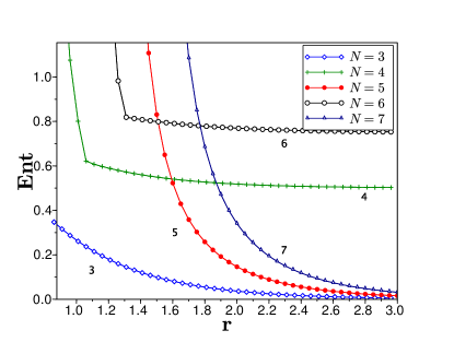
Figure 14: (Color online) Genuine $N$-partite entanglement for the CV symmetric EPR-type state II of Fig. 11. Labels as in previous figures. Green solid line corresponds to the Criterion (10) with $N=4$; diamonds correspond to the single inequality Criteria (8), with the values $g_{i}$, $h_{i}$ given in Table 5.

For the symmetric EPR state II (Figure 11), it is not as easy to find a simple single inequality that will signify four-partite entanglement, over the entire range of $r$. The problem is as follows: For large $r$, on examining the generation scheme and defining the modes as in Section V.A, we note: for $BS2$, $a_{2^{\prime}}=\frac{1}{\sqrt{2}}(a_{2}+a_{3})$; for the third $BS$, $a_{1^{\prime}}=\frac{1}{\sqrt{2}}(a_{1}-a_{4})$ and hence $x^{\prime}_{1}=\frac{1}{\sqrt{2}}(x_{1}-x_{4})$ and $p^{\prime}_{1}=\frac{1}{\sqrt{2}}(p_{1}-p_{4})$. This means that the original EPR correlation corresponding to $[\Delta(x^{\prime}_{1}-x^{\prime}_{2})]^{2}\rightarrow 0$, $[\Delta(p^{\prime}_{1}+p^{\prime}_{2})]^{2}\rightarrow 0$, becomes $[\Delta((x_{1}-x_{4})-(x_{2}+x_{3}))]^{2}\rightarrow 0$, $[\Delta(p_{1}-p_{4}+p_{2}+p_{3})]^{2}\rightarrow 0$. Thus, we can see that these latter two variances will vanish, implying violation of the inequality

$$I \geq 4$$ (41)

where $I=[\Delta((x_{1}-x_{4})-(x_{2}+x_{3}))]^{2}+[\Delta(p_{1}-p_{4}+p_{2}+p_{3})]^{2}$. Now, we see that this violation will negate biseparability of the state with respect to the bipartitions $123-4$, $124-3$, $431-2$, $234-1$, $14-23$ (use the proof of Criterion (8)). However, the violation cannot negate the bipartitions $12-34$ and $13-24$, and cannot therefore demonstrate genuine four-partite entanglement. Despite that, our analysis with general coefficients using Criterion (8) reveals that all the bipartitions can be negated, for a different choice of coefficients $g_{i}$ and $h_{i}$, provided $r\rightarrow\infty$. This means we can use the single inequality to detect genuine $N$-partite entanglement, for highly squeezed inputs, as shown in Fig. 14.

VIII.2 Criteria for four-partite entanglement using the van Loock-Furusawa inequalities

We can apply the approach of Result (1) (Eq. (13)) and Criterion (1) to derive a criterion for genuine four-partite entanglement, based on summation of van Loock-Furusawa inequalities. We will consider four systems, and label the set of bipartitions $123-4$, $124-3$, $234-1$, $134-2$, $12-34$, $13-24$, $14-23$ by $k=1,..,7$. Van Loock and Furusawa derived a set of six inequalities cvsig , that if violated eliminate biseparability with respect to certain bipartitions:

$$B_{I}\equiv[\Delta(x_{1}-x_{2})]^{2}\,\,\,\,\,\,\,\,\,\,\,\,\,\,\,\,\,\,\,\,\,\,\,\,\,\,\,\,\,\,\,\,\,\,\,\,\,\,\,\,\,\,\,\,\,\,\,\,\,\,\,\,$$

$${}+[\Delta(p_{1}+p_{2}+g_{3}p_{3}+g_{4}p_{4})]^{2} \geq 4$$

$$B_{II}\equiv[\Delta(x_{2}-x_{3})]^{2}\,\,\,\,\,\,\,\,\,\,\,\,\,\,\,\,\,\,\,\,\,\,\,\,\,\,\,\,\,\,\,\,\,\,\,\,\,\,\,\,\,\,\,\,\,\,\,\,\,\,\,\,$$

$${}+[\Delta(g_{1}p_{1}+p_{2}+p_{3}+g_{4}p_{4})]^{2} \geq 4$$

$$B_{III}\equiv[\Delta(x_{1}-x_{3})]^{2}\,\,\,\,\,\,\,\,\,\,\,\,\,\,\,\,\,\,\,\,\,\,\,\,\,\,\,\,\,\,\,\,\,\,\,\,\,\,\,\,\,\,\,\,\,\,\,\,\,\,\,\,$$

$${}+[\Delta(p_{1}+g_{2}p_{2}+p_{3}+g_{4}p_{4})]^{2} \geq 4$$

$$B_{IV}\equiv[\Delta(x_{3}-x_{4})]^{2}\,\,\,\,\,\,\,\,\,\,\,\,\,\,\,\,\,\,\,\,\,\,\,\,\,\,\,\,\,\,\,\,\,\,\,\,\,\,\,\,\,\,\,\,\,\,\,\,\,\,\,\,$$

$${}+[\Delta(g_{1}p_{1}+g_{2}p_{2}+p_{3}+p_{4})]^{2} \geq 4$$

$$B_{V}\equiv[\Delta(x_{2}-x_{4})]^{2}\,\,\,\,\,\,\,\,\,\,\,\,\,\,\,\,\,\,\,\,\,\,\,\,\,\,\,\,\,\,\,\,\,\,\,\,\,\,\,\,\,\,\,\,\,\,\,\,\,\,\,\,$$

$${}+[\Delta(g_{1}p_{1}+p_{2}+g_{3}p_{3}+p_{4})]^{2} \geq 4$$

$$B_{VI}\equiv[\Delta(x_{1}-x_{4})]^{2}\,\,\,\,\,\,\,\,\,\,\,\,\,\,\,\,\,\,\,\,\,\,\,\,\,\,\,\,\,\,\,\,\,\,\,\,\,\,\,\,\,\,\,\,\,\,\,\,\,\,\,\,$$

$${}+[\Delta(p_{1}+g_{2}p_{2}+g_{3}p_{3}+p_{4})]^{2} \geq 4$$

(42)

where $g_{i}$ is an arbitrary real number. Van Loock and Furusawa showed that violation of any three of these inequalities will negate that the system can be in one of the possible biseparable states, that we denote by $\rho_{k}$ . The violation of any three inequalities will thus signify full four-partite inseparability. A similar set of inequalities is derived for the case of arbitrary $N$.

As we have seen, this is not enough to negate that the system could be in a mixture of the biseparable states $\rho_{k}$. However, we can extend the proof of Criterion (1), to show that sufficiently strong violations of the inequalities (as is predicted by CV GHZ states) will confirm genuine $4$-partite entanglement.

Criterion (9): Four systems are genuinely four-partite entangled if the inequality

$$\sum_{J=1}^{6}B_{J}\geq 12$$ (43)

is violated, where $B_{J}\geq 4$, $J=I,II,...,VI$, are the van Loock-Furusawa inequalities (42).For the figures, we define for this criterion, $Ent=(\sum_{J=1}^{6}B_{J})/12$.

Proof: As for Criterion (1), we begin by assuming a mixture $\rho_{BS}=\sum_{k}P_{k}\rho_{k}$ where $\rho_{k}$ is a density operator with the bipartition indexed by $k=1,2,....7$. Van Loock and Furusawa showed that four of the biseparable states $\rho_{k}$ predict any particular one of the inequalities, because four of the biseparable states $\rho_{k}$ have separability with respect to the two systems specified by the subscripts of the positions $x$ measured in the inequality. We can write

$$B_{I}\geq\sum_{k=1}^{7}P_{k}B_{I,k}\geq 4(P_{3}+P_{4}+P_{6}+P_{7})$$

and similarly $B_{II}\geq 4(P_{2}+P_{4}+P_{5}+P_{6})$, $B_{III}\geq 4(P_{2}+P_{3}+P_{5}+P_{7})$, $B_{IV}\geq 4(P_{1}+P_{2}+P_{6}+P_{7})$, $B_{V}\geq 4(P_{1}+P_{4}+P_{5}+P_{7})$, $B_{VI}\geq 4(P_{1}+P_{3}+P_{5}+P_{6})$. We see that $\sum_{J}B_{J}\geq 12(P_{1}+P_{2}+P_{3}+P_{4}+P_{5}+P_{6}+P_{7})$, which gives the result. $\square$

For symmetric systems where the $B_{J}$ are equal, we will require $B_{J}<2$ ($50$% reduction of the vacuum noise level) in order to achieve Criterion (9). Predictions are given in Figure 5, for the CV GHZ state generated by the scheme of Figure 9. A very high degree of entanglement is possible as $r\rightarrow\infty$. The genuine $4$-partite entanglement of the CV GHZ state is detectable using the Criterion (9), for moderate values of $r$, though greater squeezing is required than for the $N=3$ case. The method can be extended to higher $N$, once the van Loock-Furusawa inequalities are known. We note the genuine $4$-partite entanglement of the EPR-type states is not effectively detected by this criterion.

VIII.3 Criteria for $4$-partite entanglement using summation of inequalities

Let us return to the symmetric EPR-type state II, of Figure 11. We now use the approach of Result (1) and Criterion (1) to tailor a criterion for this state, using the van Loock-Furusawa inequalities. For $N=4$, we have seen that the inequality (41) given by $I\geq 4$ will negate bipartitions $123-4$, $124-3$, $431-2$, $234-1$, $14-23$ but not the bipartitions $12-34$ and $13-24$. On the other hand, the van Loock-Furusawa inequality $B_{II}\geq 4$ will negate the bipartitions $12-34$, $13-24$, $124-3$, $431-2$. It has been shown in Ref. seiji that the EPR-type state II does violate the van Loock-Furusawa inequality, by a small amount. We can prove the following:

Criterion (10): The violation of the inequality

$$I+B_{II}\geq 4$$ (44)

is sufficient to prove genuine $4$-partite entanglement. For the figures, we define for this criterion, $Ent=(I+B_{II})/4$.

Proof: If we assume a mixture $\rho_{BS}=\sum_{k}P_{k}\rho_{k}$ where $\rho_{k}$ is a density operator biseparable across the bipartition indexed by $k=1,2,....7,$ then $I\geq 4(P_{1}+P_{2}+P_{3}+P_{4}+P_{5}$) whereas $B_{II}\geq 4(P_{2}+P_{3}+P_{6}+P_{7})$. Hence for any biseparable state the inequality will hold. $\square$

The combined inequality (44) can indeed be used to detect the genuine $4$-partite entanglement of the EPR-type state II, and the predictions are given in the Figure 14.

IX Conclusion

This paper examines how to confirm genuine multi-partite entanglement using continuous variable (that is, quadrature phase amplitude) measurements, pointing out that the approach pioneered by van Loock and Furusawa is not in itself sufficient in realistic situations, where one needs to exclude all mixed state models. The criteria are based on the scaled position and momentum observables of the quantized harmonic oscillator, and thus could also be used to detect the position and momentum entanglement associated with quantum mechanical oscillators, as done for bipartite entanglement in the recent experiment of Ref. optomech .

We have presented a general strategy for deriving criteria to detect genuine $N$-partite entanglement. Further, we present specific criteria and algorithms for the detection of the genuine $N$-partite entanglement of CV GHZ and EPR-type states that have been realized (or proposed) experimentally. In the GHZ case, we show that genuine tripartite entanglement could be confirmed for noise reductions at $2/3$ the level necessary to violate the standard van Loock-Furusawa inequalities. We also present specific predictions for higher $N$, and consider the effect of transmission losses which could be important to quantum communication applications. A more significant limitation in terms of detecting the genuine multipartite entanglement in a laboratory is likely to be the degree of impurity of the initial squeezed inputs. This effect has not been addressed in this paper, but has been studied in part in Ref. seiji2 .

For three parties, we also present criteria for genuine tripartite steering. This corresponds to a type of entanglement giving a multipartite EPR paradox. In that case, any single party can be “steered” by the other two, which means that entanglement can be confirmed between the two groups, even when the group of two parties (or their devices) cannot be trusted to perform proper quantum measurements. This form of entanglement is likely to be useful to multiparty one-sided device-independent quantum cryptography.

Appendix

IX.1 Proof of the relation (4)

Let us assume that the system is described by the mixture $\rho_{km,n}=\sum_{i}\eta_{i}^{(n)}\rho_{km}^{i}\rho_{n}^{i}$. Then on using the Cauchy Schwarz inequality, we find

$$(\Delta u)^{2}(\Delta v)^{2} \geq [\sum_{i}\eta_{i}^{(n)}(\Delta u)_{i}^{2}][\sum_{i}\eta_{i}^{(n)}(\Delta v)_{i}^{2}]$$ (45)

$$\geq [\sum_{i}\eta_{i}^{(n)}(\Delta u)_{i}(\Delta v)_{i}]^{2},$$

where $(\Delta u)_{i}(\Delta v)_{i}$ is the product of the variances for a pure product state of type $\psi_{km}\psi_{n}$ denoted by $i$. Generally, let us consider a system in a product state of type $\psi_{a}\psi_{b}$ and define the linear combinations $x_{a}+gx_{b}$ and $p_{a}+gp_{b}$ of the operators $x_{a}$, $p_{a}$ and $x_{b}$, $p_{b}$ for the systems described by wavefunctions $\psi_{a}$ and $\psi_{b}$ respectively. It is always true that the variances for such a product state satisfy $[\Delta(x_{a}+gx_{b})]^{2}=(\Delta x_{a})^{2}+g^{2}(\Delta x_{b})^{2}$ and $[\Delta(p_{a}+gp_{b})]^{2}=(\Delta p_{a})^{2}+g^{2}(\Delta p_{b})^{2}$. This implies that

$$[\Delta(x_{a}+gx_{b})]^{2}[\Delta(p_{a}+gp_{b})]^{2} = [(\Delta x_{a})^{2}+g^{2}(\Delta x_{b})^{2}]$$

$$\times[(\Delta p_{a})^{2}+g^{2}(\Delta p_{b})^{2}]$$

$$\geq [\Delta x_{a}\Delta p_{a}+g^{2}\Delta x_{b}\Delta p_{b}]^{2}$$

where we use that for any real numbers $x$ and $y$, $x^{2}+y^{2}\geq 2xy$. We can apply this result to deduce that for a product state of type $\psi_{km}\psi_{n}$, it is true that $(\Delta u)_{i}(\Delta v)_{i}\geq[\Delta(h_{k}x_{k}+h_{m}x_{m})][\Delta(g_{k}p_{k}+g_{m}p_{m})]+|h_{n}g_{n}|(\Delta x_{n})(\Delta p_{n})\geq|h_{k}g_{k}+h_{m}g_{m}|+|h_{n}g_{n}|$. $\square$

IX.2 Proof of the product version of the van Loock-Furusawa inequalities Eq. (LABEL:eq:threeineq-1)

For $S_{I}$, we have the condition $h_{1}=-h_{2}=g_{1}=g_{2}=1$ and $h_{3}=0$. Using the result (4), we see that the states $\rho=\sum_{i}\eta_{i}^{(2)}\rho_{13}^{i}\rho_{2}^{i}$ and $\rho=\sum_{i}\eta_{i}^{(1)}\rho_{23}^{i}\rho_{1}^{i}$ satisfy $S_{I}\geq 2$, while the state $\rho=\sum_{i}\eta_{i}^{(3)}\rho_{12}^{i}\rho_{3}^{i}$ gives $S_{I}\geq 0$. Similarly, we have $h_{2}=-h_{3}=g_{2}=g_{3}=1$ and $h_{1}=0$ for $S_{II}$. The states $\rho=\sum_{i}\eta_{i}^{(3)}\rho_{12}^{i}\rho_{3}^{i}$ and $\rho=\sum_{i}\eta_{i}^{(2)}\rho_{13}^{i}\rho_{2}^{i}$ satisfy $S_{II}\geq 2$ while the state $\rho=\sum_{i}\eta_{i}^{(1)}\rho_{23}^{i}\rho_{1}^{i}$ gives $S_{II}\geq 0$. Lastly, the conditions $h_{1}=-h_{3}=g_{1}=g_{3}=1$ and $h_{2}=0$ for $S_{III}$ give $S_{III}\geq 2$ for the states $\rho=\sum_{i}\eta_{i}^{(3)}\rho_{12}^{i}\rho_{3}^{i}$ and $\rho=\sum_{i}\eta_{i}^{(1)}\rho_{23}^{i}\rho_{1}^{i}$, and $S_{III}\geq 0$ for $\rho=\sum_{i}\eta_{i}^{(2)}\rho_{13}^{i}\rho_{2}^{i}$. $\square$

IX.3 Proof of Criterion (2)

Consider any mixture of the form Eq. (1). We can use the result (12) to write $S_{I}\geq P_{1}S_{I,1}+P_{2}S_{I,2}+P_{3}S_{I,3}\geq P_{1}S_{I,1}+P_{2}S_{I,2}$ where $S_{I,k}$ ($k=1,2,3$) is the value of $S_{I}$ predicted for the component $k$ of the mixture. Now we know that the first two states of the mixture satisfy the inequality, $S_{I}\geq 2$. Hence, for any mixture $S_{I}\geq 2(P_{1}+P_{2})$. Similarly, $S_{II}\geq 2(P_{2}+P_{3})$ and $S_{III}\geq 2(P_{1}+P_{3})$. Then we see that since $\sum_{k=1}^{3}P_{k}=1$, for any mixture it must be true that $S_{I}+S_{II}+S_{III}\geq 4$. $\square$

IX.4 Mixed bipartite entangled states that are fully tripartite inseparable

Consider the mixed biseparable state of the type given by Shalm et al. shalm-1

$$\rho_{BS}^{c}=\frac{1}{2}\rho_{12}\rho_{3}+\frac{1}{2}\rho_{23}\rho_{1}$$ (47)

This mixed state satisfies the van Loock- Furusawa criteria for full tripartite inseparability but, being a mixture of biseparable states, is not genuinely tripartite entangled. Here $\rho_{12}$ and $\rho_{23}$ are two-mode squeezed states defined by $\rho_{km}=|\psi_{km}\rangle\langle\psi_{km}|$ where $|\psi_{km}\rangle=(1-x^{2})^{1/2}\sum_{n=0}^{\infty}x^{n}|n\rangle_{k}|n\rangle_{m}$. Here, $|n\rangle_{k}$ are the number states of mode $k$, $x=\tanh(r)$ and $r\geq 0$ is the squeeze parameter that determines the amount of two-mode squeezing (entanglement) between the modes $k$ and $m$. The $\rho_{j}$ are single mode vacuum squeezed states, with squeeze parameter denoted by $r$. The component $\rho_{12}\rho_{3}$ can violate the inequality $B_{I}\geq 4$, while $\rho_{23}\rho_{1}$ can violate the inequality $B_{II}\geq 4$. It is straightforward to show on selecting $g_{1}=g_{3}=g$ that $\rho_{BS}$ can violate both inequalities. This demonstrates the full inseparability of the biseparable mixture, by way of the van Loock-Furusawa inequalities. Unless one can exclude mixed states, therefore, further criteria are needed to detect genuine tripartite entanglement.

IX.5 Proof of Criterion (6)

This follows from the result Eq. (4). Using Eq. (4), we see that the bipartition given by $12-3$ implies $\Delta u\Delta v\geq|g_{3}h_{3}|+|h_{1}g_{1}+h_{2}g_{2}|,$ the bipartition $13-2$ implies $\Delta u\Delta v\geq|g_{2}h_{2}|+|h_{1}g_{1}+h_{3}g_{3}|,$ and the bipartition $23-1$ implies $\Delta u\Delta v\geq|g_{1}h_{1}|+|g_{2}h_{2}+h_{3}g_{3}|.$ Thus, we see that any mixture Eq. (1) will imply Eq. (20). $\square$

IX.6 Proof of the relations Eq. (25) and Eq. (26) for EPR steering criteria

For the special sort of bipartition $\{km,n\}_{s}$, only system $n$ is constrained to be a quantum state. Letting $u=h_{k}x_{k}+h_{m}x_{m}+h_{n}x_{n}$ and $v=g_{k}p_{k}+g_{m}p_{m}+g_{n}p_{n}$, we show that always

$$[\Delta(h_{k}x_{k}+h_{m}x_{m}+h_{n}x_{n})]^{2}+[\Delta(g_{k}p_{k}+g_{m}p_{m}+g_{n}p_{n})]^{2}$$

$$\geq\sum_{i}\eta_{i}\{(h_{n}^{2}\Delta x_{n}^{2})_{i}+\Delta(h_{m}x_{m}+h_{k}x_{k})^{2}$$

$$+(g_{n}^{2}\Delta p_{n}^{2})_{i}+\Delta(g_{m}p_{m}+g_{k}p_{k})^{2}\},$$

where we follow Ref. hoftake and use that for a mixture, the variance cannot be less than the average of the variance of the components. Because the state of systems $k$ and $m$ is not assumed to be a quantum state, there is only the assumption of non-negativity for the associated variances. The single system $n$, however, is constrained to be a quantum state, and therefore its moments satisfy the uncertainty relation, which implies $(\Delta x_{n})^{2}+(\Delta p_{n})^{2}\geq 2$. Hence, if we assume that system $k,m$ cannot steer $n$, the following inequality will hold:

$$(\Delta u)^{2}+(\Delta v)^{2}\geq 2|h_{n}g_{n}|.$$ (48)

The product relation follows similarly. $\square$

IX.7 Proof of Criteria (1s) and (2s)

We assume the hybrid LHS model associated with Eq. (24) is valid. Since then $B_{I}$ is the sum of two variances of a system in a probabilistic mixture, we can write $B_{I}\geq P_{1}B_{I,1}+P_{2}B_{I,2}+B_{I,3}\geq P_{1}B_{I}+P_{2}B_{2}$ where $B_{I,n}$ denotes the prediction for $B_{I}$ given the system is in the bipartition $\{km,n\}_{s}$. Now we know that the first two states of the mixture satisfy the inequality, $B_{I}\geq 2$. Hence, for any mixture $B_{I}\geq 2(P_{1}+P_{2})$. Similarly, $B_{II}\geq 2(P_{2}+P_{3})$ and $B_{III}\geq 2(P_{1}+P_{3})$. Then we see that since $\sum_{k=1}^{3}P_{k}=1$, for any mixture it must be true that $B_{I}+B_{II}+B_{III}\geq 4$. Hence tripartite genuine steering is confirmed when this inequality is violated. and Similarly, for the hybrid LHS model, $S_{I}\geq P_{1}S_{I,1}+P_{2}S_{I,2}+P_{3}S_{I,3}\geq P_{1}S_{I,1}+P_{2}S_{I,2}$ where $S_{I,n}$ ($n=1,2,3$) is the value of $S_{I}$ predicted given the system is in the bipartition $\{km,n\}_{s}$. Now we know that the first two states of the mixture satisfy the inequality, $S_{I}\geq 1$. Hence, for any mixture $S_{I}\geq P_{1}+P_{2}$. Also, $S_{II}\geq P_{2}+P_{3}$ and $S_{III}\geq P_{1}+P_{3}$, which implies $S_{I}+S_{II}+S_{III}\geq 2$. $\square$

IX.8 Proof of Criteria (3s) and (4s)

Proof: First, we assume the system is described by the bipartition $\{12,3\}_{st}$. Using Eq. (25) with $u=x_{1}-\frac{(x_{2}+x_{3})}{\sqrt{2}}$ and $v=p_{1}+\frac{(p_{2}+p_{3})}{\sqrt{2}}$, this gives the constraint $(\Delta u)^{2}+(\Delta v)^{2}\geq 1$. Similarly, the bipartition $\{13,2\}_{st}$ gives $(\Delta u)^{2}+(\Delta v)^{2}\geq 1$, and the bipartition $\{23,1\}_{st}$ gives $(\Delta u)^{2}+(\Delta v)^{2}\geq 2$. Thus, all bipartitions satisfy $(\Delta u)^{2}+(\Delta v)^{2}\geq 1$. Using the result Eq. (10), for the system in a probabilisitc mixture where moments are given as Eq. (24), we can say that $(\Delta u)^{2}+(\Delta v)^{2}\geq 1$. Thus, genuine tripartite steering is confirmed if this inequality is violated. Using Eq. (26) for the bipartition $\{12,3\}_{st}$, it is also true that $\Delta u\Delta v\geq\frac{1}{2}$, and similarly for bipartition $\{13,2\}_{st}$. For bipartition $\{23,1\}_{st}$ we find $\Delta u\Delta v\geq 1$. Then again, for any mixture, using Eq. (12), we deduce Criterion (4s). $\square$

IX.9 Optimising the Criterion (8)

We describe the algorithm to compute the gains ($g,h$) used in the Figures based on Criterion (8), for the GHZ and asymmetric and symmetric EPR-type states. The variances $(\Delta u)^{2}$ and $(\Delta v)^{2}$ on the left-side of the inequality (37) can be expanded in terms of covariance matrix elements of the inputs (following Ref. cvsig ), which can then be computed for the relevant CV quantum state. We select $h_{i}=h$ and $g_{i}=g$ for for $i\geq 2$. The choice of $g,h$ values was obtained by setting $\frac{d}{dh}(\Delta u)^{2}=0$ and $\frac{d}{dg}(\Delta v)^{2}=0$. For the CV GHZ state, expanding we have

$$(\Delta u)^{2}=\frac{1}{N}[(N-1)^{2}h^{2}+2h(N-1)+1](\Delta x_{1}^{(in)})^{2}$$

$$+\frac{(N-1)}{N}[h^{2}-2h+1](\Delta x_{2}^{(in)})^{2}$$

$$(\Delta v)^{2}=\frac{1}{N}[(N-1)^{2}g^{2}+2g(N-1)+1](\Delta p_{1}^{(in)})^{2}$$

$$+\frac{(N-1)}{N}[g^{2}-2g+1](\Delta p_{2}^{(in)})^{2}$$ (49)

which gives on differentiation, the choice of

$$h=-\frac{(\Delta x_{1}^{(in)})^{2}-(\Delta x_{2}^{(in)})^{2}}{(\Delta x_{2}^{(in)})^{2}+(N-1)(\Delta x_{1}^{(in)})^{2}}$$

$$g=-\frac{(\Delta p_{1}^{(in)})^{2}-(\Delta p_{2}^{(in)})^{2}}{(\Delta p_{2}^{(in)})^{2}+(N-1)(\Delta p_{1}^{(in)})^{2}}$$ (50)

Here, $(\Delta x_{1}^{(in)})^{2}=e^{2r}$ , $(\Delta x_{2}^{(in)})^{2}=e^{-2r}$ , $(\Delta p_{1}^{(in)})^{2}=e^{-2r}$, and $(\Delta p_{2}^{(in)})^{2}=e^{2r}$ are the variances for the two inputs to BS1, as depicted in Figure 9. The superscript $(in)$ denotes the input modes. For the $N=4$ configuration at large $r$, we see that $g=1$ and $h=-1/3$. In general, for $g,h$ values satisfying $|gh|\leq 1$, $gh<0$, $1-2gh\geq 1$, we see that the right-side of Criterion (8) reduces to $2[1+(N-3)gh]$. Identical procedures are used to obtain the gains for the asymmetric EPR-type state I of Figure 10. They are given as:

$$h=-\frac{(\Delta x_{1}^{(in)})^{2}-(\Delta x_{2}^{(in)})^{2}}{\sqrt{(N-1)}[(\Delta x_{2}^{(in)})^{2}+(\Delta x_{1}^{(in)})^{2}]}$$

$$g=-\frac{(\Delta p_{1}^{(in)})^{2}-(\Delta p_{2}^{(in)})^{2}}{\sqrt{(N-1)}[(\Delta p_{2}^{(in)})^{2}+(\Delta p_{1}^{(in)})^{2}]}$$ (51)

For the $N=4$ configuration at large $r$, we see that $g=1/\sqrt{3}$ and $h=-1/\sqrt{3}$. For the symmetric EPR-type state II of Figure 11, the analytical expressions depend on whether the number of parties that are involved is even or odd. However, the algorithm to compute these gains is otherwise identical.

References

- (1) D. Liebfried et al., Nature, 438, 639 (2005); T. Monz et al., Phys. Rev. Lett. 106, 130506 (2011); C. Gross, T. Zibold, E. Nicklas, J. Esteve, and M. K. Oberthaler, Nature (London) 464, 1165 (2010); M. F. Riedel, P. Böhi, Y. Li, T.W. Hänsch, A. Sinatra, and P. Treutlein, Nature (London) 464, 1170 (2010).
- (2) W. Wieczorek, R. Krischeck, N. Kiesel, P. Michelberger, G. Tóth, and H. Weinfurter, Phys. Rev. Lett. 103, 020504 (2009); C. Y. Lu, X. Q. Zhou, O. Gühne, W. B. Gao, J. Zhang, Z. S. Yuan, A. Goebel, T. Yang, and J. W. Pan, Nature Physics 3, 91 (2007); J. W. Pan, D. Bouwmeester, M. Daniell, H. Weinfurter, and A. Zeilinger, Nature 403, 515 (2000); M. Bourennane, M. Eibl, C. Kurtsiefer, S. Gaertner, H. Weinfurter, O. Gühne, P. Hyllus, D. Bruß, M. Lewenstein, and A. Sanpera, Phys. Rev. Lett. 92, 087902 (2004); S. B. Papp, K. S. Choi, H. Deng, P. Lougovski, S. J. van Enk, and H. J. Kimble, Science 324, 764 (2009).
- (3) J. Lavioe, R. Kaltenbaek, and K. J. Resch, New J. Phys 11, 073051 (2009); H. X. Lu, J. Q. Zhao, X. Q. Wang, and L. Z. Cao , Phys. Rev. A 84, 012111 (2011).
- (4) L. K. Shalm, D. R. Hamel, Z. Yan, C. Simon, K. J. Resch, and T. Jennewein, Nature Phys. 9, 19-22 (2013).
- (5) T. Aoki, N. Takei, H. Yonezawa, K. Wakui, T. Hiraoka, A. Furusawa, and P. van Loock, Phys. Rev. Lett. 91, 080404 (2003).
- (6) A. S. Coelho, F. A. S. Barbosa, K. N. Cassemiro, A. S. Villar, M. Martinelli, and P. Nussenzveig, Science 326, 823 (2009).
- (7) S. Armstrong, J. F. Morizur, J. Janousek, B. Hage, N. Treps, P. K. Lam, and H. A. Bachor, Nature Commun. 3, 1026 (2012).
- (8) G. Svetlichny, Phys. Rev. D 35, 3066 (1987).
- (9) D.M. Greenberger, M.A. Horne, and A. Zeilinger, in “Bell’s Theorem, Quantum Theory, and Conceptions of the Universe” (Kluwer, Dordrecht, 1989), p. 69.
- (10) D. Collins, N. Gisin, S. Popescu, D. Roberts, and V. Scarani, Phys. Rev. Lett. 88, 170405 (2002).
- (11) M. Seevinck and G. Svetlichny, Phys. Rev. Lett. 89, 060401 (2002).
- (12) T. Moroder, J. D. Bancal, Y. C. Liang, M. Hofmann, and O. Gühne, Phys. Rev. Lett. 111, 030501 (2013); O. Gühne and G. Toth, Phys. Rep. 474, 1 (2009); O. Gühne and M. Seevinck, New J. Phys. 12, 053002 (2010); B. Jungnitsch, T. Moroder, and O. Gühne, Phys. Rev. Lett. 106, 190502 (2011); R. Horodecki, P. Horodecki, M. Horodecki, and K. Horodecki, Rev. Mod. Phys. 81, 865 (2009); M. Horodecki, P. Horodecki, and R. Horodecki, Phys. Lett. A 223, 1 (1996); B. M. Terhal, Phys. Lett. A 271, 319 (2000); M. Lewenstein, B. Kraus, J. I. Cirac, and P. Horodecki, Phys. Rev. A 62, 052310 (2000); D. Bruß, J. I. Cirac, P. Horodecki, F. Hulpke, B. Kraus, M. Lewenstein, and A. Sanpera, J. Mod. Opt. 49, 1399 (2002).
- (13) J. Bancal, N. Gisin, Y. C. Liang, and S. Pironio, Phys. Rev. Lett. 106, 250404 (2011).
- (14) J. Eisert and M. Plenio, Int. J. Quant. Inf. 1, 479 (2003).
- (15) C. Weedbrook, S. Pirandola, R. García-Patrón, N. J. Cerf, T. C. Ralph, J. H. Shapiro, and S. Lloyd, Rev. Mod. Phys. 84, 621 (2012).
- (16) S. L. Braunstein and P. van Loock, Rev. Mod. Phys. 77, 513 (2005).
- (17) M. D. Reid, P. D. Drummond, W. P. Bowen, E. G. Cavalcanti, P. K. Lam, H. A. Bachor, U. L. Anderson, and G. Leuchs, Rev. Mod. Phys. 81, 1727 (2009).
- (18) A. Furusawa, J. L. Sørensen, S. L. Braunstein, C. A. Fuchs, H. J. Kimble, and E. S. Polzik, Science 282, 706 (1998); W. P. Bowen, N. Treps, B. C. Buchler, R. Schnabel, T. C. Ralph, H. A. Bachor, T. Symul, and P. K. Lam, Phys. Rev. A 67, 032302 (2003); S. Takeda, T. Mizuta, M. Fuwa, P. van Loock, and A. Furusawa, Nature 500, 315 (2013); L. Steffen, Y. Salathe, M. Oppliger, P. Kurpiers, and M. Baur , Nature, 500, 319 (2013).
- (19) V. Scarani, H. B. Pasquinucci, N. J. Cerf, M. Dušek, N. Lütkenhaus, and M. Peev, Rev. Mod. Phys. 81, 1301 (2009).
- (20) Z. Y. Ou, S. F. Pereira, H. J. Kimble, and K. C. Peng, Phys. Rev. Lett. 68, 3663 (1992).
- (21) M. D. Reid, Phys Rev. Lett. 84, 2765 (2000).
- (22) S. G. Hofer, W. Wieczorek, M. Aspelmeyer, and K. Hammerer, Phys. Rev. A 84, 052327 (2011); V. Giovannetti, S. Mancini, and P. Tombesi, Europhys. Lett. 54, 559 (2001); C. Genes, A. Mari, P. Tombesi, and D. Vitali, Phys. Rev. A 78, 032316 (2008).
- (23) P. Hyllus and J. Eisert, New Journal of Physics 8, 51 (2008).
- (24) G. Giedke, B. Kraus, M. Lewenstein, and J. I. Cirac, Phys. Rev. A 64, 052303 (2001); Phys. Rev. Lett. 87, 167904 (2001).
- (25) G. Adesso and F. Illuminati, J. Phys. A 40, 7821 (2007).
- (26) P. van Loock and A. Furusawa, Phys. Rev. A 67, 052315 (2003).
- (27) S. Armstrong, M. Wang, R.Y. Teh, Q. Gong, Q. He, J. Janousek, H. Bachor, M.D. Reid and P.K. Lam, to appear in Nature Physics.
- (28) Q. Y. He and M. D. Reid, Phys. Rev. Lett. 111, 250403 (2013).
- (29) P. van Loock and S. L. Braunstein, Phys. Rev. Lett. 84, 3482 (2000). P. van Loock and S.L. Braunstein, Phys. Rev. A 63, 022106 (2001).
- (30) A. Einstein, B. Podolsky, and N. Rosen, Phys. Rev. 47, 777 (1935).
- (31) H. M. Wiseman, S. J. Jones, and A. C. Doherty, Phys. Rev. Lett. 98, 140402 (2007); S. J. Jones, H. M. Wiseman, and A. C. Doherty, Phys. Rev. A 76, 052116 (2007); E. G. Cavalcanti, S. J. Jones, H. M. Wiseman, and M. D. Reid, Phys. Rev. A. 80, 032112 (2009).
- (32) B. Opanchuk, L. Arnaud, and M. D. Reid, Phys. Rev. A 89, 062101 (2014).
- (33) C. Branciard, E. G. Cavalcanti, S. P. Walborn, V. Scarani, and H. M. Wiseman, Phys. Rev. A 85, 010301(R) (2012).
- (34) M. Hillery, V. Bužek, and A. Berthiaume, Phys. Rev. A 59, 1829 (1999).
- (35) M. D. Reid, Phys. Rev. A 40, 913 (1989).
- (36) B. L. Schumaker and C. M. Caves, Phys. Rev. A 31, 3093 (1985).
- (37) A. Heidmann, R. J. Horowicz, S. Reynaud, E. Giacobino, C. Fabre, and G. Camy, Phys Rev. Lett. 59, 2555 (1987).
- (38) R. E. Slusher, L. W. Hollberg, B. Yurke, J. C. Mertz, and J. F. Valley, Phys. Rev. Lett. 55, 2409 (1985); M. D. Reid and D. F. Walls, Phys. Rev. A33, 4465 (1986).
- (39) A. S. Villar, M. Martinelli, C. Fabre, and P. Nussenzveig, Phys. Rev. Lett. 97, 140504 (2006).
- (40) H. F. Hofmann and S. Takeuchi, Phys. Rev. A 68, 032103 (2003).
- (41) S.M. Tan, Phys. Rev. A 60 2752 (1999).
- (42) V. Giovannetti, S. Mancini, D. Vitali, and P. Tombesi, Phys. Rev. A 67, 022320 (2003); B. Opanchuk, Q. Y. He, M. D. Reid, and P. D. Drummond, Phys. Rev. A 86, 023625 (2012); S. Kiesewetter, Q. Y. He, P. D. Drummond, and M. D. Reid, Phys. Rev. A 90, 043805 (2014).
- (43) L. Duan, G. Giedke, J. I. Cirac, and P. Zoller, Phys. Rev. Lett. 84, 2722 (2000).
- (44) M. K. Olsen, A. S. Bradley, and M. D. Reid, Journ Phys B: At. Mol. and Opt. 39, 2515 (2006); J. F. Wang, J. T. Sheng, S. N. Zhu, and M. Xiao, J. Opt. Soc. Am. B 30, 2130 (2013); M. Delanty and K. Ostrikov, Eur. Phys. J. D 67, 193 (2013).
- (45) J. S. Bell, Physics 1, 195 (1964).
- (46) R. Gallego, L. E. Würflinger, A. Acín, and M. Navascués, Phys. Rev. Lett. 109, 070401(2012); J. Bancal, J. Barrett, N. Gisin, and S. Pironio, Phys. Rev. A 88, 014102 (2013).
- (47) E. G. Cavalcanti, Q. Y. He, M. D. Reid, and H. M. Wiseman, Phys. Rev. A 84, 032115 (2011).
- (48) M.D. Reid, Phys. Rev. A 88, 062108 (2013); W. Bowen, R. Schnabel, P. K. Lam, and T. C. Ralph, Phys. Rev. Lett. 90, 043601 (2003).
- (49) T. A. Palomaki, J. D. Teufel, R. W. Simmonds, and K. W. Lehnert, Science 342, 710 (2013).