SCIPP 13/15
Small Field Inflation and the Spectral Index
Milton Bose, Michael Dine, Angelo Monteux and Laurel Stephenson Haskins
Santa Cruz Institute for Particle Physics and
Department of Physics,
Santa Cruz CA 95064
It is sometimes stated that in hybrid inflation; sometimes that it predicts . A number of authors have consider aspects of Planck scale corrections and argued that they affect these predictions. Here we consider these systematically, describing the situations which can yield , and the extent to which this result requires additional tuning.
1 Introduction
In [1], it was argued that, with some very mild assumptions about genericity, we can characterize small field inflation quite simply. First, it was argued that the effective theory should exhibit an approximate (global) supersymmetry in order that there be fields light on the scale of the Hubble constant during inflation, . Then, assuming :
-
1.
The inflaton is a pseudomodulus, labeling a set of approximate ground states with spontaneously broken supersymmetry.
-
2.
The effective theory should obey a discrete symmetry in order that the cosmological constant (c.c.) be approximately zero at the end of inflation.
-
3.
At the end of inflation, the inflaton must couple through relevant or marginal operators to fields which are light with respect to the scale of the energy density during inflation, in order that the cosmological constant be small at the end of inflation. In particular, it was stressed that inflation typically ends, in the hybrid case, before the inflaton reaches the waterfall region.
So-called models of hybrid inflation[2, 3, 4, 5, 6] have in common the last feature above; in [1] it was argued that this full set of conditions should be taken as the definition of hybrid inflation.
Within such models, these authors noted general features:
-
1.
The (approximate) goldstino may or may not lie in a multiplet with the inflaton.
-
2.
The effective theory exhibits an approximate, continuous symmetry.
-
3.
Terms allowed by the discrete symmetry break the accidental continuous global symmetry and spoil inflation, unless the inflationary scale (the square of the Goldstino decay constant) is sufficiently small.
-
4.
There are further requirements on the Kähler potential in order to obtain slow roll inflation with adequate -foldings. This sets an irreducible minimum amount of fine tuning necessary to achieve acceptable inflation. This tuning grows in severity with the number of Hubble mass fields.
-
5.
In order that inflation ends with small c.c., the inflaton must couple, as noted above, to other light degrees of freedom, or must have appreciable self-couplings in the final ground state. The coupling to this extra field, or the self couplings, are fixed by the density perturbations and the inflationary scale. In the case of extra fields, the resulting structure is necessarily what is called “hybrid inflation”[3, 4, 5, 6, 2]. The spectral index, quite generally, is less than one.
In [1], it was noted that for a broad range of parameters, was typical; this is widely considered a general result of hybrid models. Recently, considering the Planck CMB temperature data supplemented by the WMAP large-scale polarization data, the Planck collaboration has reported a value [7]:
| (1) |
And indeed, the authors of the Planck papers argued that their data excludes hybrid inflation. Within the definition outlined above, it is interesting to look more carefully at the range of allowed values of .
In this paper, we systematically consider various Planck scale corrections to the simplest version of hybrid inflation. We explain why (parametrically) the most important are the quartic corrections to the Kähler potential, and certain power law corrections to the superpotential. The former must be suppressed by an amount of order , where is the number of -foldings. The latter lead to an approximately zero c.c., supersymmetric minimum for large fields; in turn this means that the potential has a local maximum (saddle). This gives rise to a variant of “hilltop inflation”[8]; we will see that the initial conditions need not be substantially tuned in order that one obtain adequate -foldings and . If the superpotential has coefficient scaled by a suitable power of and a dimensionless coefficient of order one, one obtains a prediction of the scale of inflation. The scale depends on the index of a symmetry, and ranges from about GeV to GeV.
In the next section, we review the simplest hybrid model, and recall the prediction . In section 3, we classify the various Planck scale corrections to the simplest hybrid model. In section 4, we consider the implications of the leading superpotential corrections for inflation, explaining why one obtains the structure of hilltop inflation. In section 5, we present numerical results for these models. In section 6, we suggest that predictions might arise if inflation is connected with supersymmetry breaking. In section 7, we conclude by considering possible observable consequences of this picture.
2 Hybrid Models and Effects
The simplest model of hybrid inflation contains two chiral superfields, and , with superpotential
| (2) |
If one imposes, as is usually done, a continuous symmetry under which the charges of and are respectively 2 and zero, this superpotential is the most general permitted by symmetries. Classically, the theory has a moduli space,
| (3) |
on which
| (4) |
At one loop, the potential receives corrections. In the global limit:
| (5) |
If one considers only this term, one has, for the number of -foldings:
| (6) |
In this simple model, the parameter is negligible, and
| (7) |
This yields
| (8) |
This is the origin of the prediction that .
In this model, is related to by the fluctuation spectrum:
| (9) |
3 Hierarchy of Corrections
This treatment, however, is oversimplified. Already, in [4, 2], the role of higher order terms in the Kähler potential was considered. More recently, in [9], the effects of a linear term in the potential for , arising from the constant term in the superpotential (needed to account for the small cosmological constant of the present universe) has been considered. In [1], this particular contribution was treated as small, but a number of other effects were considered. So it is first worthwhile to consider the various possible corrections in powers of , and their relative importance.
First, it is generally believed that theories of gravity should not exhibit continuous global symmetries; in string theories, this is a theorem. Replacing the continuous symmetry by a discrete symmetry allows corrections of the form
| (10) |
More generally, our viewpoint will be that all terms allowed in the effective action below should appear with order one coefficients; we will assume that smaller coefficients represent a “fine tuning” of parameters. We can systematically consider types of corrections, ordered in powers of :
-
1.
Kähler potential corrections: , .
-
2.
Superpotential corrections: in addition to (and higher powers of , other fields), at some level there must be a constant in the superpotential, , to account for the smallness of the cosmological constant now.
-
3.
Supersymmetry breaking effects.
The term
| (11) |
has been noted already in [2]. In [1], precise limits on (of order , where is the number of -foldings) were discussed. It was noted that the quantum corrections of eqn. (5) only dominate over this Kähler potential correction for sufficiently small . In fact, as we will review shortly, for the simplest model, the quantum corrections never dominate unless is quite small.
Terms of sixth order or higher in in the Kähler potential are irrelevant. They lead to highly suppressed contributions to and , for example. We will be more quantitative about this question when we turn to models that can reproduce the Planck value of .
Now we turn to the various superpotential corrections. Our definition of hybrid inflation is motivated by the hypothesis that the scale of inflation is large compare to scales of supersymmetry breaking. This means, in particular, that
| (12) |
with the Hubble scale during inflation. As a result, terms in the potential arising from can be neglected during inflation. If, in fact, the actual value of is comparable to , then this term, and terms associated with supersymmetry breaking, would be important. Even for TeV, this corresponds to an inflationary energy scale well below GeV.
So finally we turn, again, to . The presence of this term in the superpotential gives rise to a supersymmetric minimum of the potential at large but parametrically smaller than . This is unlike the case, for example, of higher order corrections to the Kähler potential. As a result, this term qualitatively alters the behavior of the system, for large but not Planck scale fields. In [1] this term was used to constrain features of inflation. Requiring that it was not important during inflation constrained the scale of inflation, and lead to the prediction . To be compatible with the results from Planck, however, it is clearly necessary that inflation occur in a region near the local maximum (as in “Hilltop inflation”[8]). We will explore this in the next section.
4 Hybrid Inflation and
Including , it is first important that the system not flow towards the supersymmetric minimum. Indeed, for an intermediate range of field values, there are corrections to the potential (5) of the form
| (13) |
For negative , this leads to a maximum, for
| (14) |
To obtain suitable inflation, it is necessary that be smaller than this at the beginning. But, given eqn. (9), except for very large , is smaller than the “waterfall value”,
| (15) |
As a result of these considerations, the simplest (and rather standard) model of hybrid inflation (allowing for ) does not appear suitable. In [1], a simple modification was suggested with two fields, and , with couplings at the renormalizable level:
| (16) |
The theory, classically, has two flat directions, one with large , one with large . As in the previous model, in order that inflation occur, the Kähler potential must be tuned so that at least one of the fields or , has mass small compared to the Hubble constant during inflation, . To obtain a workable model, we require that be the light field. This amounts to requiring that in the Kähler potential term
| (17) |
should be close to unity. The waterfall regime is now at smaller value of the inflaton field , , and hybrid inflation can be driven by the quantum and discrete symmetry corrections.
Assuming a discrete symmetry, there are a variety of possible higher dimension terms which might appear in depending on the transformation properties of the fields. We will consider a term of the form
| (18) |
Alternatively, a term proportional to , for example, corrects the potential for if there is a term in the Kähler potential
| (19) |
The allowed values of depend on the discrete charge assignments of the fields. If is not too large, its effects are dramatic.
Such terms, again, lead to a supersymmetric minimum of the potential at large (with ), and again give rise, for positive , to a maximum of the potential for at field strength generically large compared to but small compared to .
Proceeding as before, using the superpotential and Kähler corrections in eqns. (16)–(18), we can compute the number of -foldings and the slow roll parameters (and hence ). The potential for is now, approximately,
| (20) |
The fluctuation spectrum relates and , as before. For a given value of , the initial value of the field at -foldings is fixed. So, then, is .
To get a rough sense of scalings, we can suppose that starts very near the maximum of the potential, and that (in order to achieve ). Because at the hilltop, we will simply use the formula for normal hybrid inflation in our estimate; shortly we will check the accuracy of this numerically, and see that this leads to an order one error. Then one finds that
| (21) |
For particular values of , we can compute and : taking and , this gives GeV and . For , one obtains GeV, and . The scale grows slowly with , reaching GeV at and GeV for . In general, these results scale with as:
| (22) |
We discuss numerical studies of this problem in the next section. But the lesson here is that, for fixed values of , and for a given , the scale of inflation, , is fixed to a narrow range.
5 Numerical Studies of Small Field Inflation
Denoting the real part of the field by , the potential in eqn. (20) becomes
| (23) |
where we have included in the numerical factor coming from the field redefinition. It will be handy to denote the hilltop position by , and to investigate how close has to be to in order to successfully have 50–60 -foldings of inflation.
For a given , the parameters of the two field model are readily enumerated: , , , and . Given knowledge of these, we can compute the observable predictions of the inflationary model, to be compared with the Planck collaboration results [7]:
-
1.
The number of -foldings . To solve the horizon and flatness problems, it must be . In our numerical treatment, we will assume the range of 50–60 -foldings.
-
2.
The slow roll parameters , which result in the spectral index . The measured value by the Planck collaboration is
-
3.
The density perturbation spectrum , whose amplitude is a function of . Planck measurements translate to .
We can, in principle, compute the tensor to scalar ratio , but in all such models this will be unobservably small. In general, as said in the previous section, quantifies the Kähler correction independent from the discrete symmetry, and is already required to be small, while the dependence on is weak. In the following we will set , .
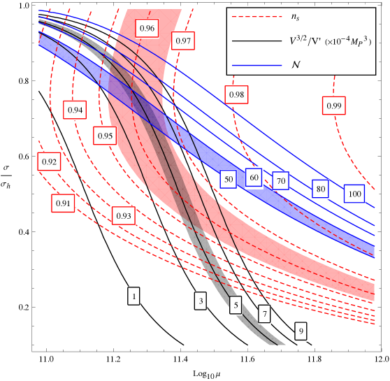
Given the potential (23), the expression for the number of -foldings involves an integral that can be computed numerically. With a analysis, for each given , we set the three remaining parameters by fitting the experimental values of . For example, in Fig. 1, where we set and to its best-fit value, we show how the allowed ranges for each experimental quantity intersect at specific values of and .
In Table 1, we give the best-fit values of , with the corresponding uncertainties for from 4 to 12. There is no fine-tuning associated with the inflaton being close to the hilltop value, as the allowed values for are in the range –. For small , the coupling is tuned to be small. In the last column, we show how close to unity has to be for the Kähler correction not to overcome the discrete symmetry correction. As is already fine-tuned to be of order in order not to spoil inflation, we conclude that there is another mild tuning which operates to keep close to 1.
For , the initial value of the field is GeV, just a factor of 10 below . For larger , it is not possible to accomodate within the framework of small field inflation. Even for this large value of the field, the tensor-to-scalar ratio is predicted to be small:
| (24) |
6 Incorporating Supersymmetry Breaking
The picture of small field inflation we have developed up to now assumes that the scale of inflation is large compared to the scale of supersymmetry breaking, i.e. that . This is the origin of the requirement that the superpotential should vanish and supersymmetry be unbroken, to a good approximation, at the end of inflation. But one might consider the possibility that . A higher scale of is suggested by the observed Higgs mass and supersymmetry exclusions. In addition, for small values of , we have obtained small values of . So it is interesting to consider the possibility that the the scale of inflation is comparable to .
For example we can modify the models we have studied, to give them an O’Raifeartaigh like structure, adding to the superpotential of eqn. (2) a coupling
| (25) |
Provided
| (26) |
supersymmetry is broken, in a state with . It is interesting that in this case, inflation ends without ever passing into a “waterfall” regime. As we have stressed, the so-called waterfall is indeed not the distinguishing feature of hybrid inflation.
A different approach has been pursued in [10]. Again, it is assumed that the scale of inflation is not too much different than the scale of supersymmetry breaking. One writes a theory of a single field, , and does not require an unbroken symmetry at the end of inflation. Instead, one assumes that the negative contribution to the cosmological constant arising from the vev of the superpotential is cancelled by some supersymmetry breaking dynamics. To constrain the form of the superpotential, one still assumes a discrete symmetry. It is necessary, as in hybrid inflation, to tune the Kähler potential so that the term is small. The superpotential takes the form:
| (27) |
while the quartic term in the Kähler potential must be quite small. The resulting model is of the hilltop type. The potential exhibits a local maximum at the origin, and the initial value of the field must lie quite close to the maximum (compared to the distance of the origin from the minimum). Inflation occurs in a region very close to the origin in field space (defined by an unbroken symmetry). The field then settles into a minimum with small cosmological constant and broken supersymmetry and symmetry. The model can produce the requisite number of -foldings and fluctuation spectrum, without introducing an extremely small number analogous to of eqn. (2). However, it predicts too small a value of ,
| (28) |
To obtain a spectral index consistent with Planck, it is necessary to introduce a small and well-tuned constant in the superpotential, which the authors denote , and is of order (in Planck units). There are other issues, such as a possible gravitino problem and overproduction of dark matter, but these can readily be solved by introducing additional matter coupled to the inflaton.
Both approaches, then, seem viable, and have the potential to relate supersymmetry breaking dynamics to inflationary dynamics. Each requires certain tunings.
7 Conclusions: Predictions and Observable Consequences for Low Energy Physics
The results from Planck pose challenges for models of small field inflation. It has been said that they rule out “hybrid inflation.” Here, following [1], we have carefully defined models of hybrid inflation as models in which inflation occurs on a pseudomoduli space, with supersymmetry and an symmetry approximately restored at the end of inflation. We have assumed a discrete symmetry, and have considered the importance of corrections to the superpotential and Kähler potential. For initial values of the field far from the local maximum of the potential, one predicts a spectral index inconsistent with Planck. To obtain , it is necessary that the field start near the local maximum, though this condition is not severely tuned. For symmetry with , the scale of inflation is rather low, and we considered the possibility that . In this case, the dynamics of inflation might be closely tied to the scale of supersymmetry breaking, and there is some chance that aspects of the physics of inflation could be studied in accelerator experiments.
We have noted that, in this case, the assumption of an unbroken symmetry and unbroken supersymmetry at the end of inflation might be relaxed, and compared the hybrid models with those of [10]. Each of these models can reproduce the data, and involves very small parameters and tunings. The fact that many models with such features can reproduce the basic data of inflation raises, as always, the question of whether there is any way they might be testable or falsifiable. We would argue that the best hope is connecting inflation with the dynamics responsible for supersymmetry breaking. It will be particularly interesting to explore dynamical supersymmetry breaking (and generation of scales) in this framework.
Acknowledgements: We thank Andrei Linde and Fuminobu Takahashi for discussions. This work supported in part by the U.S. Department of Energy.
References
- [1] Michael Dine and Lawrence Pack. Studies in Small Field Inflation. JCAP, 1206:033, 2012.
- [2] Andrei D. Linde and Antonio Riotto. Hybrid inflation in supergravity. Phys.Rev., D56:1841–1844, 1997.
- [3] Andrei D. Linde. Hybrid inflation. Phys.Rev., D49:748–754, 1994.
- [4] Edmund J. Copeland, Andrew R. Liddle, David H. Lyth, Ewan D. Stewart, and David Wands. False vacuum inflation with Einstein gravity. Phys.Rev., D49:6410–6433, 1994.
- [5] G.R. Dvali, Q. Shafi, and Robert K. Schaefer. Large scale structure and supersymmetric inflation without fine tuning. Phys.Rev.Lett., 73:1886–1889, 1994.
- [6] David H. Lyth and Antonio Riotto. Particle physics models of inflation and the cosmological density perturbation. Phys.Rept., 314:1–146, 1999.
- [7] P.A.R. Ade et al. Planck 2013 results. XXII. Constraints on inflation. 2013.
- [8] Lotfi Boubekeur and David.H. Lyth. Hilltop inflation. JCAP, 0507:010, 2005.
- [9] Constantinos Pallis and Qaisar Shafi. Update on Minimal Supersymmetric Hybrid Inflation in Light of PLANCK. Phys.Lett., B725:327–333, 2013.
- [10] Fuminobu Takahashi. New inflation in supergravity after Planck and LHC. 2013.