On the asymptotics of dimers on tori

Abstract.

We study asymptotics of the dimer model on large toric graphs. Let $\mathbb{L}$ be a weighted $\mathbb{Z}^{2}$-periodic planar graph, and let $\mathbb{Z}^{2}E$ be a large-index sublattice of $\mathbb{Z}^{2}$. For $\mathbb{L}$ bipartite we show that the dimer partition function $\text{Z}_{E}$ on the quotient $\mathbb{L}/(\mathbb{Z}^{2}E)$ has the asymptotic expansion

$$\text{Z}=\exp\{A\,\mathbf{f}_{0}+\text{{fsc}}+o(1)\}$$

where $A$ is the area of $\mathbb{L}/(\mathbb{Z}^{2}E)$, $\mathbf{f}_{0}$ is the free energy density in the bulk, and fsc is a finite-size correction term depending only on the conformal shape of the domain together with some parity-type information. Assuming a conjectural condition on the zero locus of the dimer characteristic polynomial, we show that an analogous expansion holds for $\mathbb{L}$ non-bipartite. The functional form of the finite-size correction differs between the two classes, but is universal within each class. Our calculations yield new information concerning the distribution of the number of loops winding around the torus in the associated double-dimer models.

1. Introduction

Dimer systems have been studied since the 1960s when they were introduced to model close-packed diatomic molecules, and research on them has flourished with a renewed vigor since the 1990s (see e.g. [MR2198850]).

A dimer configuration on a graph $\mathcal{G}=(\mathcal{V},\mathcal{E})$ is a perfect matching on $\mathcal{G}$: that is, a subset of edges $\mathfrak{m}\subseteq\mathcal{E}$ such that every vertex $v\in\mathcal{V}$ is covered by exactly one edge of $\mathfrak{m}$; for this reason $\mathfrak{m}$ is also referred to as a dimer cover. If $\mathcal{G}$ is a finite undirected graph equipped with non-negative edge weights $(\nu_{e})_{e\in\mathcal{E}}$, a probability measure on dimer covers is given by

$$\mathbb{P}_{\mathcal{G}}(\mathfrak{m})\equiv\frac{\nu_{\mathcal{G}}(\mathfrak{m})}{\text{Z}_{\mathcal{G}}},\quad\text{with }\nu_{\mathcal{G}}(\mathfrak{m})\equiv\prod_{e\in\mathfrak{m}}\nu_{e}\text{ and }\text{Z}_{\mathcal{G}}\equiv\sum_{\mathfrak{m}}\nu_{\mathcal{G}}(\mathfrak{m}).$$

The non-normalized measure $\nu_{\mathcal{G}}$ is the dimer measure on the $\nu$-weighted graph $\mathcal{G}$. The normalizing constant $\text{Z}_{\mathcal{G}}$ is the associated dimer partition function, with $\log\text{Z}_{\mathcal{G}}$ the free energy and $|\mathcal{V}|^{-1}\log\text{Z}_{\mathcal{G}}$ (free energy per vertex) the free energy density.

An ordered pair of independent dimer configurations gives (by superposition) a double-dimer configuration, consisting of even-length loops and doubled edges. The double-dimer partition function is $\mathcal{Z}_{\mathcal{G}}=(\text{Z}_{\mathcal{G}})^{2}$. Double-dimer configurations on planar graphs are closely related to the Gaussian free field [MR1872739, arXiv:1105.4158].

1.1. Square lattice dimer partition function

Kasteleyn, Temperley, and Fisher [Kasteleyn19611209, MR0136398, MR0136399] showed how to compute the dimer partition function $\text{Z}_{\mathcal{G}}$ on a finite planar graph $\mathcal{G}$ as the Pfaffian of a certain signed adjacency matrix, now known as the Kasteleyn matrix. For graphs embedded on a torus or other low-genus surface, $\text{Z}_{\mathcal{G}}$ can be computed by combining a small number of Pfaffians [Kasteleyn19611209, galluccio-loebl, MR1750896]; we provide further background in §2.1. Using this method, Kasteleyn [Kasteleyn19611209] showed that on the unweighted square lattice, both the $m\times n$ rectangle and $m\times n$ torus have asymptotic free energy density

$$\mathbf{f}_{0}\equiv\lim_{\begin{subarray}{c}m,n\to\infty,\\ mn\text{ even}\end{subarray}}(mn)^{-1}\log\text{Z}_{\mathcal{G}}=G/\pi,$$

where $\smash{G\equiv\sum_{j\geq 0}(-1)^{j}/(2j+1)^{2}=0.915965594\ldots}$ is Catalan’s constant. (If $mn$ is odd, clearly $\text{Z}_{\mathcal{G}}=0$.) In the case of $m$ and $n$ both even, Fisher [MR0136399] calculated the free energy of the $m\times n$ rectangle to be given more precisely by

$$\begin{array}[]{rl}\log\text{Z}&=mn\,\mathbf{f}_{0}-2(m+n)\,\mathbf{f}_{1}+O(1),\quad\text{with}\\ \mathbf{f}_{1}&=\smash{\tfrac{1}{4}}\log(1+2^{1/2})-\smash{\tfrac{1}{2}}G/\pi\end{array}$$

— the second term in the expansion of $\log\text{Z}$ is linear in the rectangle perimeter, so we interpret $\mathbf{f}_{1}$ as the surface free energy density while $\mathbf{f}_{0}$ is the bulk free energy density.

Ferdinand [ferdinand] refined the calculation further for both rectangle and torus, finding a constant-order correction term which depends on both the “shape” of the region (the choice of rectangle or torus boundary conditions, as well as the aspect ratio $\smash{\smash{\tfrac{m}{n}}}$) as well as the parities of $m$ and $n$. For $mn$ even, Ferdinand found

$$\begin{array}[]{l}\log\text{Z}=mn\,\mathbf{f}_{0}+\text{(perimeter)}\,\mathbf{f}_{1}+\text{(corners)}\,\mathbf{f}\lrcorner+\text{{fsc}}^{\mathrm{topology}}_{(-1)^{m+n}}(\smash{\tfrac{n}{m}})+o(1)\\ =\begin{cases}mn\,\mathbf{f}_{0}+\text{{fsc}}^{\mathrm{tor}}_{(-1)^{m+n}}(\smash{\tfrac{n}{m}})+o(1),&\text{($m\times n$ torus);}\\ mn\,\mathbf{f}_{0}+2(m+n)\,\mathbf{f}_{1}+4\mathbf{f}\lrcorner+\text{{fsc}}^{\mathrm{rect}}_{(-1)^{m+n}}(\smash{\tfrac{n}{m}})+o(1)&\text{($m\times n$ rectangle)}\end{cases}\end{array}$$ (1)

where $\mathbf{f}\lrcorner$ is a constant which may be interpreted as the free energy per corner, and the four functions $\text{{fsc}}^{\mathrm{tor}}_{\pm 1},\text{{fsc}}^{\mathrm{rect}}_{\pm 1}$ are explicit analytic functions of the aspect ratio $\smash{\nicefrac{{n}}{{m}}}$. These functions fsc are called the finite-size corrections to the free energy: they contain information about long-range properties of the dimer system (see e.g. [PhysRevLett.56.742, privman1990finite, cardy1996scaling]). Figure 1 shows these finite-size corrections for the $m\times n$ torus. We shall see (Figure 4) that if we expand our consideration slightly to all near-rectilinear tori — tori which are rotated with respect to the coordinate axis, or which deviate slightly from being perfectly rectangular — then in fact seven fsc curves arise in the limit.

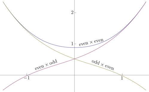
Figure 1. Unweighted square lattice dimers. Finite-size corrections fsc for rectilinear $m\times n$ tori, shown as a function of logarithmic aspect ratio $\log(n/m)$. Curves are labeled according to parity of $(m,n)$.

Kasteleyn, Fisher, and Ferdinand also carried out these calculations for the weighted square lattice where the horizontal edges receive weight $a$ while the vertical edges receive weight $b$. In this setting they found (for $mn$ even)

$$\log\text{Z}=mn\,\mathbf{f}_{0}|_{a,b}+(\text{perimeter})\,\mathbf{f}_{1}|_{a,b}+(\text{corners})\,\mathbf{f}\lrcorner|_{a,b}+\text{{fsc}}^{\mathrm{topology}}_{(-1)^{m+n}}(\smash{\tfrac{nb}{ma}})+o(1)$$ (2)

where the free energy coefficients $\mathbf{f}_{0},\mathbf{f}_{1},\mathbf{f}\lrcorner$ depend on the weights $a,b$ in a complicated manner, but the finite-size correction $\smash{\text{{fsc}}^{\mathrm{topology}}_{(-1)^{m+n}}(\smash{\tfrac{nb}{ma}})}$ is the same function as appearing in the expansion (1) for the unweighted square lattice, now applied to the “effective” aspect ratio $\smash{\tfrac{nb}{ma}}$. In this sense the finite-size corrections are seen to be robust to the particulars of the model.

Finite-size corrections for square lattice dimers have also been explicitly computed on the cylinder [MR1227270, eq. (46)] [PhysRevE.67.066114], Möbius band [MR1227270, eq. (48)] [PhysRevE.67.066114], and Klein bottle [PhysRevE.67.066114]. In each of these topologies, for each given choice of side length parities, the finite-size correction is an analytic function of the aspect ratio [PhysRevE.67.066114]. See [MR2194994, MR2280327] for a discussion of these finite-size corrections in the context of logarithmic conformal field theory.

1.2. Characteristic polynomial and spectral curve

In this article we consider dimer systems defined on two broad classes of critically weighted $\mathbb{Z}^{2}$-periodic planar lattices — rather loosely, a bipartite and a non-bipartite class. We assume throughout that the lattices are connected, with each edge occurring with positive probability. Within each class, we compute an asymptotic expansion of the dimer free energy on large toric quotient graphs — including “skew” or “helical” (non-rectilinear) tori — and explicitly determine the finite-size correction.

On non-bipartite lattices, the finite-size correction depends on a single parameter $\tau$ in the complex upper half-plane describing the conformal shape of the domain — $\smash{\nicefrac{{\tau}}{{i}}}$ generalizes the “effective aspect ratio” $\smash{\tfrac{nb}{ma}}$ appearing in (2). On bipartite lattices, the correction depends further on whether the finite torus is globally bipartite or non-bipartite, as well as on a phase parameter $(\zeta,\xi)\in\mathbb{T}^{2}$ which generalizes the signs $((-1)^{m},(-1)^{n})$ appearing in (2). The functional form of the correction is universal within each class.

More precisely, the bipartite and non-bipartite graph classes which we consider throughout this paper are characterized by algebraic conditions on the dimer characteristic polynomial. This is a certain Laurent polynomial $P(z,w)$, whose definition depends only on the combinatorics of the fundamental domain, the $1\times 1$ toric quotient of the $\mathbb{Z}^{2}$-periodic graph.

On the unit torus $\mathbb{T}^{2}\equiv\{(z,w)\in\mathbb{C}:|z|=|w|=1\}$, the characteristic polynomial $P(z,w)$ is non-negative. Many large-scale quantities of interest in the dimer model can be computed from $P$: for example the free energy per fundamental domain is given by half the logarithmic Mahler measure

$$\mathbf{f}_{0}\equiv\smash{\tfrac{1}{2}}\iint_{\mathbb{T}^{2}}\log P(z,w)\,\frac{dz}{2\pi iz}\,\frac{dw}{2\pi iw}.$$ (3)

Edge-edge correlations are obtained from the Fourier transform of $P(z,w)^{-1}$ [MR1473567].

Criticality in dimer models is characterized by the intersection of the spectral curve

$$\{(z,w)\in\mathbb{C}^{2}:P(z,w)=0\},$$

with the unit torus $\mathbb{T}^{2}$. Dimer models on bipartite graphs have been quite deeply understood, in part via the classification of the spectral curve as a simple Harnack curve [MR2215138, MR2219249, MR2099145]. The bipartition of the graph gives a natural factorization $P(z,w)=Q(z,w)Q(z^{-1},w^{-1})$ with $Q$ a real polynomial, so that the factors $Q(z,w)$ and $Q(z^{-1},w^{-1})$ are complex conjugates for $(z,w)\in\mathbb{T}^{2}$ (see §2.2). It is known that if the zero set of $Q$ on $\mathbb{T}^{2}$ is non-empty, then it consists of a pair of complex conjugate zeroes — which either are distinct, or coincide at a real root of $Q$. In the case of distinct zeroes, or zeroes coinciding at a real root at which $Q$ has a node, the model is critical or liquid, with polynomial decay of correlations. (A node is a point $(z_{0},w_{0})$ at which the polynomial is a product of two distinct lines $(b_{1}(z-z_{0})+c_{1}(w-w_{0}))(b_{2}(z-z_{0})+c_{2}(w-w_{0}))$ plus higher-order terms.) In all other cases the model is off-critical, and belongs (depending on the geometry of the spectral curve) either to a gaseous (exponential decay of correlations) or frozen (no large-scale fluctuations) phase.

Far less is known about the spectral curves of non-bipartite dimer systems. In this setting it is conjectured that the characteristic polynomial $P(z,w)$ is either non-vanishing on the unit torus, or is vanishing to second order at a single real node which is one of the four points $(\pm 1,\pm 1)$. This conjecture has been proved for the Fisher lattice with edge weights corresponding to any bi-periodic ferromagnetic Ising model on the square lattice [arXiv:1008.3936]. For lattices satisfying this condition one can show (see [MR2215138]) that frozen phases do not exist: when the spectral curve is disjoint from the unit torus the model is gaseous (off-critical), and when it intersects at a real node the model is liquid (critical). In this paper we assume this condition and illustrate its implications for critical dimer systems.

1.3. Statement of results

Let $\mathbb{L}$ be a weighted $\mathbb{Z}^{2}$-periodic quasi-transitive (that is, the quotient $\mathbb{L}/\mathbb{Z}^{2}$ is finite) planar graph. We consider dimers on large toric quotients of $\mathbb{L}$, as follows: let ${\text{End}_{+}(\mathbb{Z}^{2})}$ be the set of integer $2\times 2$ matrices

$$E\equiv\begin{pmatrix}u&v\\ x&y\end{pmatrix}\quad\quad\quad\text{with }\det E>0.$$ (4)

Any $E\in{\text{End}_{+}(\mathbb{Z}^{2})}$ defines the toric graph $\mathbb{L}_{E}\equiv\mathbb{L}/(\mathbb{Z}^{2}E)$, the quotient of $\mathbb{L}$ modulo translation by the vectors in the lattice $\mathbb{Z}^{2}E\equiv\{a(u,v)+b(x,y):a,b\in\mathbb{Z}\}$. We take asymptotics with $E$ tending to infinity while being “well-shaped” in the sense that

$$\begin{array}[]{l}\text{$\det E$ tends to infinity}\\ \hskip 10.0pt\text{while remaining within a constant factor of both $\|(u,v)\|^{2}$ and $\|(x,y)\|^{2}$.}\end{array}$$ (5)

1.3.1. Finite-size correction to the characteristic polynomial

The $1\times 1$ toric quotient $\mathbb{L}_{I}$ (with $I$ the $2$-dimensional identity matrix) is called the fundamental domain. We assume it has $k$ vertices with $k$ even: as a consequence (see §LABEL:ss:odd.general), $\mathbb{L}$ is equipped with a periodic Kasteleyn orientation in which the contour loop surrounding each face has an odd number of clockwise-oriented edges [MR0253689]. (In §LABEL:s:odd we discuss how to handle $k$ odd, for which such orientations do not exist.) The dimer characteristic polynomial $P(z,w)$ is the determinant of a certain $k$-dimensional matrix $K(z,w)$ associated with the fundamental domain, which may be considered as the discrete Fourier transform of the (infinite-dimensional) weighted signed adjacency matrix of $\mathbb{L}$. For a brief review and formal definitions see §2.1.

Of course for given $\mathbb{L}$ there is some freedom in the choice of fundamental domain: in particular any $\mathbb{L}_{E}$ may be regarded as the fundamental domain, with corresponding characteristic polynomial $P_{E}(\zeta,\xi)$ which is the determinant of a $(k\det E)$-dimensional matrix $K_{E}(\zeta,\xi)$. It can be obtained from $P(z,w)$ by the double product formula

$$P_{E}(\zeta,\xi)=\prod_{\begin{subarray}{c}z^{u}w^{v}=\zeta\\ z^{x}w^{y}=\xi\end{subarray}}P(z,w),$$ (6)

(see e.g. [MR1815214, MR1473567, MR2215138]). If the characteristic polynomial $P$ is non-vanishing on the unit torus, it is easily seen from (6) (see Theorem 2, below) that, in the limit (5), $\log P_{E}(\zeta,\xi)=(\det E)\,2\mathbf{f}_{0}+o(1)$ uniformly over $(\zeta,\xi)\in\mathbb{T}^{2}$, which readily implies (using e.g. Proposition 2.2) the free energy expansion $\log\text{Z}_{E}=(\det E)\,\mathbf{f}_{0}+o(1)$.

In this paper we compute an asymptotic expansion of $P_{E}(\zeta,\xi)$ ($\zeta,\xi\in\mathbb{T}$) in the more interesting critical case where $P(z,w)$ is vanishing to second order at nodes on the unit torus. Formally, let us say that $P$ has a positive node at $(e^{i\text{{{r}}}_{0}},e^{i\text{{{s}}}_{0}})\in\mathbb{T}^{2}$ if it is vanishing there to second order with positive-definite Hessian matrix:

$$\begin{array}[]{l}P(e^{\pi i(\text{{{r}}}_{0}+\text{{{r}}})},e^{\pi i(\text{{{s}}}_{0}+\text{{{s}}})})=\pi^{2}\langle(\text{{{r}}},\text{{{s}}}),H(\text{{{r}}},\text{{{s}}})\rangle+O(\|(\text{{{r}}},\text{{{s}}})\|^{3})\quad\text{where }\\ \displaystyle H=\begin{pmatrix}A_{z}&B\\ B&A_{w}\end{pmatrix}\text{ with }A_{z},A_{w}>0\text{ and }D\equiv\sqrt{A_{z}A_{w}-B^{2}}>0.\end{array}$$ (7)

In the bipartite case (see above), distinct conjugate zeroes of $Q$ correspond to positive nodes of $P$; see (21). If instead $Q$ has a real node, the Harnack property implies that this node is positive (up to global sign change). We associate to $H$ the parameter

$$\tau[H]\equiv(-B+iD)/A_{w}\in\mathbb{H}\equiv\{z\in\mathbb{C}:\operatorname{Im}z>0\}.$$ (8)

Theorem 1.

Suppose $P(z,w)$ is an analytic non-negative function defined on the unit torus $\mathbb{T}^{2}$, non-vanishing except at positive nodes $(z_{j},w_{j})$ ($1\leq j\leq\ell$) with associated Hessians $H_{j}$. Then, in the limit (5), for $\zeta,\xi\in\mathbb{T}$ we have

$$\log P_{E}(\zeta,\xi)=2(\det E)\,\mathbf{f}_{0}+\sum_{j=1}^{\ell}2\log\hyperlink{e:cf}{\bm{\Xi}}\Big{(}\frac{\zeta}{z_{j}^{u}w_{j}^{v}},\frac{\xi}{z_{j}^{x}w_{j}^{y}}\,\Big{|}\,\tau_{j}\Big{)}+O\Big{(}\frac{1}{n^{2/5}\bm{r}}\Big{)}$$ (9)

where $\mathbf{f}_{0}$ is given by (3), $\bm{r}$ is the minimum Euclidean distance between $(1,1)$ and the set of points $(\zeta/(z_{j}^{u}w_{j}^{v}),\xi/(z_{j}^{x}w_{j}^{y}))$, $\tau_{j}$ is the parameter (8) associated to the transformed Hessian $(E^{t})^{-1}H_{j}E^{-1}$, and Ξ is the explicit function (LABEL:e:cf).

In the two settings we consider (see §1.2), the spectral curve of the characteristic polynomial either intersects the unit torus at a single positive node $(z_{0},w_{0})=(\pm 1,\pm 1)$ with Hessian $H$, or at conjugate positive nodes $(z_{0},w_{0})\neq(\overline{z}_{0},\overline{w}_{0})$ with the same Hessian $H$ (see (21)). These conjugate nodes may occur at the same point, in which case $P$ vanishes to fourth order; however in this case we can still treat each node separately in Theorem 1. In either case we define

$$\begin{array}[]{rl}\displaystyle\tau_{E}\equiv\frac{x+y\,\tau[H]}{u+v\,\tau[H]}=\tau[(E^{t})^{-1}HE^{-1}]\in\mathbb{H}&\quad\text{the \emph{conformal shape of $\mathbb{L}_{E}$};}\\[12.0pt] (\zeta_{E},\xi_{E})\equiv(e^{\pi i\text{{{r}}}_{E}},e^{\pi i\text{{{s}}}_{E}})\equiv(z_{0}^{u}w_{0}^{v},z_{0}^{x}w_{0}^{y})\in\mathbb{T}^{2}&\quad\text{the \emph{domain phase of $\mathbb{L}_{E}$}.}\end{array}$$ (10)

where $\text{{{r}}}_{E},\text{{{s}}}_{E}$ are chosen to lie in the interval $(-1,1]$. (In the case of two distinct nodes, for most purposes it suffices to take the phase to be defined modulo complex conjugation. For one of our results, Theorem LABEL:t:gaussian, we specify a distinction between the nodes to have a more explicit statement.)

1.3.2. Finite-size correction to the dimer partition function

By the method of Pfaffians [Kasteleyn19611209, galluccio-loebl, MR1750896] (see also [cimasoni-reshetikhin]), the dimer partition function on $\mathbb{L}_{E}$ is a signed combination of the four square roots $P_{E}(\pm 1,\pm 1)^{1/2}$:

$$\text{Z}_{E}=\smash{\tfrac{1}{2}}[\pm P_{E}(+1,+1)^{1/2}\pm P_{E}(+1,-1)^{1/2}\pm P_{E}(-1,+1)^{1/2}\pm P_{E}(-1,-1)^{1/2}]$$

(a review is given in §2.1; see in particular Proposition 2.2). In §LABEL:s:fsc we explain how to choose the signs to deduce from Theorem 1 the finite-size correction to the dimer partition function for the two classes of critically weighted graphs described above:

Theorem 2.

If the spectral curve $\{P(z,w)=0\}$ is disjoint from the unit torus, then $\log\text{Z}_{E}=(\det E)\,\mathbf{f}_{0}+o(1)$.

1. If the spectral curve intersects the unit torus at a single real positive node with associated Hessian $H$, then

   $$\log\text{Z}_{E}=(\det E)\,\mathbf{f}_{0}+\hyperlink{FSC_1}{\text{{{fsc}}}_{1}}(\tau_{E})+o(1)$$

   where $\tau_{E}$ is as in (10), and $\hyperlink{FSC_1}{\text{{{fsc}}}_{1}}\equiv\log\hyperlink{FSC_1}{\text{{{FSC}}}_{1}}$ with

   $$\textstyle\hyperlink{FSC_1}{\text{{{FSC}}}_{1}}(\tau)\equiv\smash{\tfrac{1}{2}}\sum_{\zeta,\xi=\pm 1}\hyperlink{e:cf}{\bm{\Xi}}(\zeta,\xi|\tau).$$

2. Suppose the fundamental domain is bipartite, with dimer characteristic polynomial $P(z,w)=Q(z,w)\,Q(\smash{\nicefrac{{1}}{{z}}},\smash{\nicefrac{{1}}{{w}}})$ non-vanishing on $\mathbb{T}^{2}$ except at distinct conjugate positive nodes $(z_{0},w_{0})\neq(\overline{z}_{0},\overline{w}_{0})$ with associated Hessian $H$. Then

   $$\log\text{Z}_{E}=(\det E)\,\mathbf{f}_{0}+\hyperlink{FSC_2}{\text{{{fsc}}}_{2}}(\zeta_{E},\xi_{E}|\tau_{E})+o(1)$$

   where $\tau_{E},\zeta_{E},\xi_{E}$ are as in (10), and $\hyperlink{FSC_2}{\text{{{fsc}}}_{2}}\equiv\log\hyperlink{FSC_2}{\text{{{FSC}}}_{2}}$ with

   $$\textstyle\hyperlink{FSC_2}{\text{{{FSC}}}_{2}}(\zeta,\xi|\tau)\equiv\smash{\tfrac{1}{2}}\sum_{z,w=\pm 1}\hyperlink{e:cf}{\bm{\Xi}}(z\zeta,w\xi|\tau)^{2}$$

   which has the equivalent expression

   $$\hyperlink{FSC_2}{\text{{{FSC}}}_{2}}(e^{\pi i\text{{{r}}}},e^{\pi i\text{{{s}}}}|\tau)=\frac{\sum_{\bm{e}\in\mathbb{Z}^{2}}\exp\{-\smash{\tfrac{\pi}{2}}g_{\tau}(\bm{e}-(\text{{{s}}},-\text{{{r}}}))\}}{|\hyperlink{Dedekind}{\eta}(\tau)|^{2}(2\operatorname{Im}\tau)^{1/2}}$$ (11)

   where for $\tau\in\mathbb{H}$, $g_{\tau}$ is the quadratic form

   $$g_{\tau}(\bm{e})\equiv(\tau_{\mathrm{im}})^{-1}(e_{1}^{2}+2\tau_{\mathrm{re}}e_{1}e_{2}+|\tau|^{2}e_{2}^{2})$$ (12)

   and η is the Dedekind eta function.

3. Suppose the fundamental domain is bipartite, with dimer characteristic polynomial $P(z,w)=Q(z,w)\,Q(\smash{\nicefrac{{1}}{{z}}},\smash{\nicefrac{{1}}{{w}}})$ non-vanishing on $\mathbb{T}^{2}$ except at a single (real) root at which $Q$ has a positive node with associated Hessian $H$. Then

   $$\log\text{Z}_{E}=(\det E)\,\mathbf{f}_{0}+\hyperlink{FSC_2}{\text{{{fsc}}}_{2}}(1,1|\tau_{E})+o(1)$$

   where $\tau_{E}$ is as in (10).

4. If the spectral curve intersects the unit torus at two real positive nodes $(z_{1},w_{1})$ and $(z_{2},w_{2})$ with the same associated Hessian $H$, then

   $$\log\text{Z}_{E}=(\det E)\,\mathbf{f}_{0}+\hyperlink{FSC_3}{\text{{{fsc}}}_{3}}(\zeta_{E},\xi_{E}|\tau_{E})+o(1)$$

   where, defining $(z_{0},w_{0})\equiv(z_{1}z_{2},w_{1}w_{2})$, the parameters $\tau_{E},\zeta_{E},\xi_{E}$ are as in (10), and $\hyperlink{FSC_3}{\text{{{fsc}}}_{3}}\equiv\log\hyperlink{FSC_3}{\text{{{FSC}}}_{3}}$ with

   $$\textstyle\hyperlink{FSC_3}{\text{{{FSC}}}_{3}}(\zeta,\xi|\tau)\equiv\smash{\tfrac{1}{2}}\sum_{z,w=\pm 1}\hyperlink{e:cf}{\bm{\Xi}}(z,w|\tau)\hyperlink{e:cf}{\bm{\Xi}}(z\zeta,w\xi|\tau)$$

   We further have the simplifications

   $$\begin{array}[]{rl}\hyperlink{FSC_3}{\text{{{FSC}}}_{3}}(+1,+1|\tau)&=\hyperlink{FSC_2}{\text{{{FSC}}}_{2}}(+1,+1|\tau)\\ \hyperlink{FSC_3}{\text{{{FSC}}}_{3}}(+1,-1|\tau)&=\hyperlink{e:cf}{\bm{\Xi}}(-1,-1|\tau)\hyperlink{e:cf}{\bm{\Xi}}(-1,+1|\tau)=\hyperlink{e:cf}{\bm{\Xi}}(-1,+1|2\tau)\\ \hyperlink{FSC_3}{\text{{{FSC}}}_{3}}(-1,+1|\tau)&=\hyperlink{e:cf}{\bm{\Xi}}(-1,-1|\tau)\hyperlink{e:cf}{\bm{\Xi}}(+1,-1|\tau)=\hyperlink{e:cf}{\bm{\Xi}}(+1,-1|\smash{\nicefrac{{\tau}}{{2}}})\\ \hyperlink{FSC_3}{\text{{{FSC}}}_{3}}(-1,-1|\tau)&=\hyperlink{e:cf}{\bm{\Xi}}(-1,+1|\tau)\hyperlink{e:cf}{\bm{\Xi}}(+1,-1|\tau)=\hyperlink{e:cf}{\bm{\Xi}}(+1,-1|\smash{\tfrac{1+\tau}{2}})\end{array}$$

See Figure 5 for plots of these functions fsc1, fsc2, and fsc3. In [MR2215138, Thm. 5.1] it is shown that for bipartite graphs on tori, case d does not occur. However, for graphs on tori that are locally bipartite but not globally bipartite, such as an odd$\times$even grid on a torus, we see in Section LABEL:ss:square that this case does occur.

We emphasize again that the functional form of the finite-size correction is universal within each class: the finite-size correction Ξ to the characteristic polynomial (Theorem 1) is an explicit function depending only on the three parameters $\zeta,\xi,\tau$. Thus in Theorem 2a the graph structure enters into the correction only through $\tau$ (that is, only through the Hessian associated with the real node). In the bipartite setting (Theorem 2b, c, and d), the finite-size correction depends on the graph structure only through $\tau$ and $(\zeta_{E},\xi_{E})$.

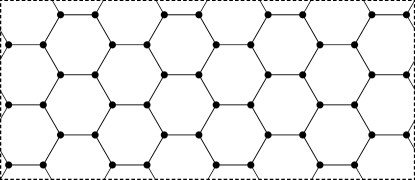
Figure 2. The $4\times 3$ toric quotient of the honeycomb graph, with effective aspect ratio $\rho=\smash{\nicefrac{{\sqrt{3}}}{{4}}}$ (also the actual aspect ratio of this geometric embedding) in the unweighted setting.

As we explain in §LABEL:ss:modular, the parameter $\tau$ has a simple interpretation as the half-period ratio of the torus with respect to its “natural” or “conformal” embedding. Consequently the finite-size corrections are invariant under modular transformations. For example, for the unweighted honeycomb graph, the $m\times n$ torus (Figure 2) has $\tau=i\rho$ where $\rho=\smash{\nicefrac{{n}}{{(m\sqrt{3})}}}$ is the effective or geometric aspect ratio.

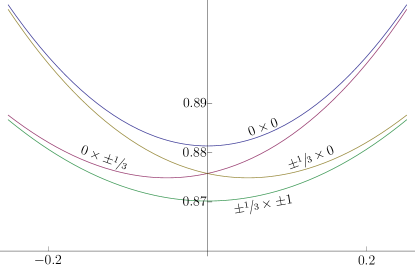
Figure 3. Unweighted honeycomb graph dimers. Finite-size corrections $\hyperlink{FSC_2}{\text{{{fsc}}}_{2}}(\zeta_{E},\xi_{E}|\tau)$ for near-rectilinear toric quotients, shown as a function of logarithmic aspect ratio $\log\rho$, labelled according to value of $(u-v,x-y)/3$ modulo $1$ (see §LABEL:ss:hex).

The domain phase parameter $(\zeta_{E},\xi_{E})$ is of a quite different nature: it generalizes the signs $(-1)^{m},(-1)^{n}$ appearing in (2), and depends sensitively on the entries of $E$. For example, for dimers on the honeycomb lattice, the finite-size correction for $m\times n$ quotients (Figure 2) was computed by Boutillier and de Tilière in the case $n\equiv 0\bmod 3$ [MR2561433]. Figure 3 shows this correction for the unweighted honeycomb lattice as a function of the logarithmic effective aspect ratio $\log\rho$, together with three other curves — one showing the different correction which applies for $n\not\equiv 0\bmod 3$, and the remaining two showing corrections which can be found on toric quotients which are nearly but not quite rectilinear. Some discussion of this is given in §LABEL:ss:hex.

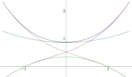
Figure 4. Unweighted square lattice dimers. Finite-size corrections fsc for near-rectilinear toric quotients, shown as a function of the logarithmic aspect ratio $\log\rho$. There are seven distinct curves, depending on parities of vectors defining the torus (see §LABEL:ss:square). (It is easy to distinguish only five of the curves, see Figure LABEL:f:torus.square.magnify for a magnified view.)

(a) $\hyperlink{FSC_1}{\text{{{fsc}}}_{1}}(\tau)$

(b) $\hyperlink{FSC_2}{\text{{{fsc}}}_{2}}(+1,e^{2\pi i/6}|\tau)$

(c) $\hyperlink{FSC_2}{\text{{{fsc}}}_{2}}(i,i|\tau)$

(d) $\hyperlink{FSC_2}{\text{{{fsc}}}_{2}}(+1,+1|\tau)=\hyperlink{FSC_3}{\text{{{fsc}}}_{3}}(+1,+1|\tau)$                                         

(e) $\hyperlink{FSC_2}{\text{{{fsc}}}_{2}}(i,+1|\tau)$

(f) $\hyperlink{FSC_2}{\text{{{fsc}}}_{2}}(+1,i|\tau)$

(g) $\hyperlink{FSC_3}{\text{{{fsc}}}_{3}}(+1,-1|\tau)$

(h) $\hyperlink{FSC_3}{\text{{{fsc}}}_{3}}(-1,+1|\tau)$

(i) $\hyperlink{FSC_3}{\text{{{fsc}}}_{3}}(-1,-1|\tau)$

Figure 5. Free energy finite-size corrections as a function of $\tau=x+iy\in\mathbb{H}$. In these plots, $-1\leq x\leq 1$ and $0<y\leq 1$, and the identically zero function is indicated by the horizontal plane. There is one fsc1 function, there are four fsc3 functions, and there is a two-parameter family of fsc2 functions. Panels (c) through (i) show the seven functions for unweighted square-grid tori; their restrictions to the pure imaginary line $\tau=i\rho$ are the curves in Figure 4 (shown there as a function of $\log\rho$). Panels (b) and (d) show two of the functions relevant to unweighted honeycomb graph tori; see Figure 3. The function shown in panel (a) is relevant to the Ising model; see Figure 8.

In the square lattice we find a similar phase sensitivity, but we find a dependence also on the global bipartiteness of the torus (for example, the $4\times 3$ torus in the square lattice is non-bipartite). As a result, for near-rectilinear tori the finite-size correction lies asymptotically on any of seven curves, Figure 4 — four curves for bipartite tori and three for nonbipartite. Further discussion of this is given in §LABEL:s:odd.

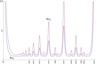
Figure 6. $\hyperlink{FSC_1}{\text{{{fsc}}}_{1}}(x+i/200)$ (blue) and $\hyperlink{FSC_2}{\text{{{fsc}}}_{2}}(1,1|x+i/200)$ (red). The local maxima in $\hyperlink{FSC_2}{\text{{{fsc}}}_{2}}(1,1|\tau)$ are twice as high as those for $\hyperlink{FSC_1}{\text{{{fsc}}}_{1}}(\tau)$.

1.3.3. Non-contractible loops on the torus

Recall that the superposition of two independent dimer covers of a planar graph $\mathcal{G}$ produces a double-dimer configuration consisting of even-length loops and doubled edges. Alternatively, a single dimer cover of $\mathcal{G}$ may be mapped to a double-dimer configuration by superposition with a fixed reference matching $\overline{\mathfrak{m}}$. It is of interest to study the non-contractible loops arising from this process on toric graphs. In addition to the finite-size corrections to the overall dimer partition functions $\text{Z}_{E}$ (Theorem 2), we are able to obtain some finer information on the distribution of the partition function between dimer covers of different homological types, as follows.

Non-contractible loops in the bipartite setting. If $\mathcal{G}$ is bipartite, a double-dimer configuration resulting from the (ordered) pair $(\mathfrak{m},\mathfrak{m}^{\prime})$ is naturally regarded as an oriented loop configuration $\mathfrak{m}\ominus\mathfrak{m}^{\prime}$, with edges from $\mathfrak{m}$ oriented black-to-white and edges from $\mathfrak{m}^{\prime}$ oriented white-to-black. We then let

$$\operatorname{\text{{{wind}}}}\mathfrak{m}\ominus\mathfrak{m}^{\prime}\equiv(\text{{{w}}}_{\mathrm{h}},\text{{{w}}}_{\mathrm{v}})\in\mathbb{Z}^{2}$$ (13)

denote the homology class (or “winding numbers”) of the oriented loop configuration.

For $m\times n$ toric quotients of the unweighted honeycomb tiling (Figure 2), it was shown in [MR2561433] that for $n\in 3\mathbb{Z}$, the winding $\operatorname{\text{{{wind}}}}\mathfrak{m}\ominus\overline{\mathfrak{m}}$ of a dimer cover $\mathfrak{m}$ with respect to a fixed reference matching $\overline{\mathfrak{m}}$ is asymptotically distributed as a pair of independent discrete Gaussians, with variances determined by the torus aspect ratio. The proof is based on a perturbative analysis of the finite-size correction, and we generalize their method to prove

Theorem 3.

In the setting of Theorem 2b, let $\mathfrak{m}_{E}$ be a fixed reference matching of $\mathbb{L}_{E}$ obtained by periodically extending a matching $\mathfrak{m}_{0}$ of the fundamental domain. Then the winding $\operatorname{\text{{{wind}}}}\mathfrak{m}\ominus\mathfrak{m}_{E}\in\mathbb{Z}^{2}$ asymptotically fluctuates as a discrete Gaussian:

$$\begin{array}[]{l}\displaystyle\mathbb{P}(\operatorname{\text{{{wind}}}}\mathfrak{m}\ominus\mathfrak{m}_{E}=\bm{e})\to\frac{\exp\{-\smash{\tfrac{\pi}{2}}(\bm{e}-\hyperlink{MuSigma}{\bm{\mu}_{E}})^{t}\hyperlink{MuSigma}{\bm{\Sigma}_{\mathrlap{E}}}^{-1}(\bm{e}-\hyperlink{MuSigma}{\bm{\mu}_{E}})\}}{\sum_{\bm{e}^{\prime}\in\mathbb{Z}^{2}}\exp\{-\smash{\tfrac{\pi}{2}}(\bm{e}^{\prime}-\hyperlink{MuSigma}{\bm{\mu}_{E}})^{t}\hyperlink{MuSigma}{\bm{\Sigma}_{\mathrlap{E}}}^{-1}(\bm{e}^{\prime}-\hyperlink{MuSigma}{\bm{\mu}_{E}})\}}\quad\text{with}\vspace{4pt}\\ \displaystyle\text{covariance }\hyperlink{MuSigma}{\bm{\Sigma}_{E}}=\frac{(E^{t})^{-1}HE^{-1}}{(\det H)^{1/2}/\det E},\quad\text{center }\hyperlink{MuSigma}{\bm{\mu}_{E}}\equiv\pm\smash{\tfrac{1}{\pi}}(\arg\xi_{E},-\arg\zeta_{E})\mod\mathbb{Z}^{2}.\end{array}$$

A more explicit version of Theorem 3 is given as Theorem LABEL:t:gaussian, stated and proved in §LABEL:s:torus.bip. Dubédat [dubedat, Thm. 7] proved a version of Theorem 3 for dimers on bipartite isoradial graphs.

Non-contractible loops in the non-bipartite setting. In the non-bipartite setting, the loop configuration $\mathfrak{m}\oplus\mathfrak{m}^{\prime}$ is not oriented, and we take the winding $\operatorname{\text{{{wind}}}}\mathfrak{m}\oplus\mathfrak{m}^{\prime}$ to be defined only as an element of $(\mathbb{Z}/2\mathbb{Z})^{2}$. In the setting of Theorem 2a, we also compute (Proposition LABEL:p:torus.nonbip) the finite-size corrections to the partition functions $\text{Z}_{E}^{\,\text{{{r}}}\text{{{s}}}}$ of the four homology classes indexed by $(\text{{{r}}},\text{{{s}}})\in\{\text{{{0}}},\text{{{1}}}\}^{2}$.

To note one particular motivation, we remark that this winding is of particular interest in the context of Ising models. On a graph $\mathcal{G}=(\mathcal{V},\mathcal{E})$ with real-valued parameters $(\beta_{e})_{e\in\mathcal{E}}$ (coupling constants), we define the associated Ising model to be the probability measure on spin configurations $\underline{\smash{\sigma}}\in\{\pm 1\}^{\mathcal{V}}$ given by

$${}^{\ddagger}{\mathbb{P}}_{\mathcal{G}}(\underline{\smash{\sigma}})\equiv\frac{1}{{}^{\ddagger}{\text{Z}}_{\mathcal{G}}}\prod_{e=(uv)\in\mathcal{E}}\exp\{\beta_{e}\sigma_{u}\sigma_{v}\}.$$

On the square lattice with vertical and horizontal coupling constants $\beta_{a}$ and $\beta_{b}$ (“Onsager’s lattice”), the bulk free energy density ${}^{\ddagger}\mathbf{f}_{0}$ was first calculated by Onsager [MR0010315]. Kasteleyn [MR0153427] and Fisher [fisher1966dimer] rederived this result by exhibiting a correspondence between the Ising model on a planar (weighted) graph $\mathcal{G}$ and the dimer model on various “decorated” versions $\mathcal{G}^{\prime}$ of $\mathcal{G}$.

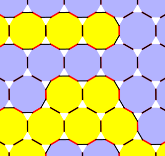
Figure 7. Fisher correspondence between the Ising model on the triangular lattice and the dimer model on the Fisher lattice. The Ising spins $\pm 1$ (yellow and blue) live on the dodecagonal faces of the Fisher lattice. The Fisher lattice is given the reference matching $\overline{\mathfrak{m}}$ consisting of all between-triangle edges (black). Take the unique dimer configuration $\mathfrak{m}$ which contains a between-triangle edge if and only if it separates like spins (red): then the loops of $\mathfrak{m}\oplus\mathfrak{m}$ trace the spin domain boundaries in the low-temperature expansion of the Ising model. The Ising and dimer partition functions are related in (14).

For instance, the Ising model on the triangular lattice with coupling constants $\beta_{a},\beta_{b},\beta_{c}$ corresponds — via its low-temperature expansion — to the dimer model on the Fisher lattice with unit weights on the within-triangle edges, and weights $(a,b,c)=(e^{2\beta_{a}},e^{2\beta_{b}},e^{2\beta_{c}})$ on the edges between triangles (Figure 7). To calculate the Ising partition function ${}^{\ddagger}{\text{Z}}_{m,n}$ on the $m\times n$ torus in the triangular lattice, take the $m\times n$ torus in the Fisher lattice, and fix the reference matching $\overline{\mathfrak{m}}$ consisting of all $(a,b,c)$-edges. Let $\text{Z}^{\,\text{{{0}}}\text{{{0}}}}[a,b,c]$ denote the partition function of dimer configurations $\mathfrak{m}$ with $\operatorname{\text{{{wind}}}}\mathfrak{m}\oplus\overline{\mathfrak{m}}=(\text{{{0}}},\text{{{0}}})$: then

$${}^{\ddagger}{\text{Z}}_{m,n}=\frac{2\cdot\text{Z}^{\text{{{0}}}\text{{{0}}}}_{m,n}[e^{2\beta_{a}},e^{2\beta_{b}},e^{2\beta_{c}}]}{\prod_{e}e^{\beta_{e}}}.$$ (14)

At $\beta_{c}=0$ ($c=1$), the Ising model on the triangular lattice reduces to the Ising model on Onsager’s lattice. Criticality for $\mathbb{Z}^{2}$-periodic Ising models has been characterized in terms of the intersection of the Fisher lattice spectral curve with the unit torus ([LiCMP, arXiv:1008.3936], see also [CDCIsing]).

Using (14) and similar correspondences, the asymptotic expansion of the Ising partition function has been computed in numerous contexts [PhysRev.185.832, Bugrij1990171, O'Brien199663, PhysRevE.65.036103, MR1690485, PhysRevE.63.026107, PhysRevE.67.065103, MR2000227]. In particular, for Onsager’s lattice on the ferromagnetic critical line

$$a+b+1=ab\quad\text{with }a=e^{2\beta_{a}}\text{ and }b=e^{2\beta_{b}},$$ (15)

the Ising free energy on $m\times n$ graphs has the expansion (compare (2))

$$\log{}^{\ddagger}{\text{Z}}_{m,n}=mn\,{}^{\ddagger}\mathbf{f}_{0}+(\text{perimeter})\,{}^{\ddagger}\mathbf{f}_{1}+(\text{corners})\,{}^{\ddagger}\mathbf{f}\lrcorner+{}^{\ddagger}\text{{fsc}}^{\mathrm{topology}}(\smash{\tfrac{n}{m}}\smash{\tfrac{a^{2}-1}{2a}})+o(1),$$

where ${}^{\ddagger}\text{{fsc}}$ is an explicit analytic function depending on the topology (rectangle, torus, cylinder, etc.) — but not on the parity of $(m,n)$. On the anti-ferromagnetic critical line

$$a^{-1}+b^{-1}+1=(ab)^{-1},$$

the finite-size correction depends also on the parity of $(m,n)$. Figure 8 shows the finite-size corrections for $m\times n$ toric quotients of the homogeneous Onsager’s lattice ($\beta_{a}=\beta_{b}=\beta$) at the critical points

$$\beta=\pm\smash{\tfrac{1}{2}}\log(\sqrt{2}+1),$$

where $\beta$ positive is ferromagnetic and $\beta$ negative is anti-ferromagnetic.

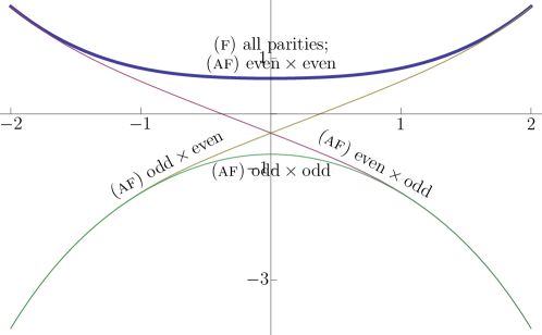
Figure 8. Square lattice critical Ising ($\beta=\smash{\tfrac{1}{2}}\log(\sqrt{2}+1)$). Finite-size corrections for $m\times n$ tori as a function of logarithmic aspect ratio $\log\rho$.

The following proposition characterizes criticality for the Fisher lattice, as well as for a superficially similar lattice, the so-called rhombitrihexagonal tiling (Figure LABEL:f:hst). The latter graph has no known correspondence with the Ising model, yet its dimer systems exhibit some similar features. Though the proposition is easy to prove and various special cases appear in the literature, we include a detailed proof in the appendix (§LABEL:s:fisher.hst) for completeness. Combined with Theorem 2a, it gives the finite-size correction for general (critical) Ising models on large toric quotients (including skew tori) of the triangular lattice and Onsager’s lattice.

Proposition 1.1.

For the Fisher graph (Figure LABEL:f:fisher) or the 3.4.6.4 graph (Figure LABEL:f:hst), the spectral curve can only intersect the unit torus at a real node, characterized by the vanishing of one of the four quantities

$$\bm{c}\begin{pmatrix}-\mathrm{Pf}\,K(+1,+1)\\ +\mathrm{Pf}\,K(+1,-1)\\ +\mathrm{Pf}\,K(-1,+1)\\ +\mathrm{Pf}\,K(-1,-1)\\ \end{pmatrix}=\begin{pmatrix}+a+b+c-abc\\ -a+b+c+abc\\ +a-b+c+abc\\ +a+b-c+abc\\ \end{pmatrix}\equiv\begin{pmatrix}\kappa_{\circ}\\ \kappa_{a}\\ \kappa_{b}\\ \kappa_{c}\end{pmatrix}$$ (16)

where $\bm{c}$ is $1$ for the Fisher graph, and $\smash{\nicefrac{{1}}{{2}}}$ for the 3.4.6.4 graph.

For dimers coming from the Ising model, such as on the Fisher graph, the node coincides with the Ising model’s critical temperature [LiCMP, CDCIsing].

We summarize the relevant background in Section 2. Theorem 2 is proved in Section LABEL:s:fsc. In Section LABEL:s:torus.bip we prove Theorem LABEL:t:gaussian, which is a stronger version of Theorem 3. In Section LABEL:s:odd we consider lattices with odd-sized fundamental domain, which provide examples for some of the cases in Theorem 2. We postpone the proof of Theorem 1 until Section LABEL:s:torus.pf, even though the proofs of Theorem 2 and LABEL:t:gaussian depend on it, since its proof is somewhat technical. Proposition 1.1 is proved in Appendix LABEL:s:fisher.hst.

Acknowledgements

We thank Cédric Boutillier and Béatrice de Tilière for several interesting conversations. This research was conducted and completed during visits of R. K. and N. S. to Microsoft Research.

2. Preliminaries

Throughout this paper, $\mathbb{L}$ denotes a $\mathbb{Z}^{2}$-periodic quasi-transitive planar graph equipped with positive edge weights.

2.1. Kasteleyn orientation and characteristic polynomial

The Kasteleyn orientation is a way of computing the dimer and double-dimer partition functions via matrix Pfaffians and determinants. The Pfaffian of a $2n\times 2n$ skew-symmetric matrix is given by

$$\mathrm{Pf}\,K\equiv\frac{1}{n!\,2^{n}}\sum_{\sigma\in S_{2n}}(\operatorname{sgn}\sigma)\prod_{j=1}^{n}K_{\sigma(2j-1),\sigma(2j)},$$ (17)

and satisfies $(\mathrm{Pf}\,K)^{2}=\det K$. If $K$ is the (skew-symmetric) weighted adjacency matrix of a finite directed graph $\mathcal{G}$, then each non-zero term in (17) corresponds to a dimer cover of $\mathcal{G}$. All the $n!\,2^{n}$ permutations $\sigma\in S_{2n}$ corresponding to the same dimer cover $\mathfrak{m}$ appear with the same sign $\operatorname{sgn}\mathfrak{m}$ in (17), so that we may write $\mathrm{Pf}\,K=\sum_{\mathfrak{m}}\,(\mathrm{Pf}\,K)_{\mathfrak{m}}$ where each matching contributes $(\mathrm{Pf}\,K)_{\mathfrak{m}}\equiv(\operatorname{sgn}\mathfrak{m})\prod_{(ij)\in\mathfrak{m}}|K_{ij}|$.

Every finite planar graph $\mathcal{G}$ can be equipped with a Kasteleyn or Pfaffian orientation, in which all dimer covers $\mathfrak{m}$ appear with the same sign $\operatorname{sgn}\mathfrak{m}$ in (17) — that is, for which $|\mathrm{Pf}\,K|$ is the dimer partition function $\text{Z}_{\mathcal{G}}$ of $\mathcal{G}$, and $\det K$ is the double-dimer partition function $(\text{Z}_{\mathcal{G}})^{2}$. A Kasteleyn orientation is given by arranging each (non-external) face to be clockwise odd, i.e. with an odd number of edges oriented in the clockwise direction; see [MR0253689, §V-D] for details.

Returning to the setting of §1.3, let $\mathbb{L}$ be a planar $\mathbb{Z}^{2}$-periodic lattice, with an even number $k$ of vertices per fundamental domain. $\mathbb{L}$ can be equipped with a periodic Kasteleyn orientation in which every face is clockwise odd (see §LABEL:ss:odd.general); this defines an infinite-dimensional weighted signed adjacency matrix (Kasteleyn matrix) $K$, with entries $K_{ij}\equiv(\mathbf{1}_{i\to j}-\mathbf{1}_{j\to i})\nu_{ij}$ for $i,j\in\mathbb{L}$. For $z,w\in\mathbb{C}$ and

$$E=\begin{pmatrix}u&v\\ x&y\end{pmatrix}\in{\text{End}_{+}(\mathbb{Z}^{2})}\,,$$

define a $(z,w)$-periodic function to be a function $f:\mathbb{L}\to\mathbb{C}$ satisfying $f(p+a(u,v)+b(x,y))=f(p)z^{a}w^{b}$ for $p\in\mathbb{L}$ and $a,b\in\mathbb{Z}$. We let

$$K_{E}(z,w)\quad\text{the ``Fourier transform of $K$ with respect to $E$''}$$ (18)

denote the action of $K$ on the (finite-dimensional) space of $(z,w)$-periodic functions. We write $K(z,w)\equiv K_{I}(z,w)\in\mathbb{C}^{k\times k}$ (where $I$ is the identity matrix) and call

$$P(z,w)\equiv\det K(z,w)\quad\text{the \emph{characteristic polynomial\/} of $\mathbb{L}$.}$$

Note that $K(z,w)^{\operatorname{t}}=-K(\smash{\nicefrac{{1}}{{z}}},\smash{\nicefrac{{1}}{{w}}})$, so $P(z,w)=P(\smash{\nicefrac{{1}}{{z}}},\smash{\nicefrac{{1}}{{w}}})$.

2.2. Bipartite characteristic polynomial

Note that in (18) the linear map $K(z,w)$ was defined without reference to a basis, which is unnecessary for defining the determinant. To consider Pfaffians of $K(z,w)$, however, we must fix a basis: from the relation $\mathrm{Pf}\,(MKM^{t})=(\det M)(\mathrm{Pf}\,K)$ it is clear that even an orthogonal change of basis can change the sign of the Pfaffian. We therefore assume a fixed ordering $1,\ldots,k$ of the vertices of the fundamental domain, and take the basis $(f_{1},\ldots,f_{k})$ where $f_{p}(q)=z^{a}w^{b}$ if $q$ is the vertex corresponding to $p$ in the $(a,b)$-translate of the fundamental domain, and $f_{p}(q)=0$ for all other $q$. For the action of $K_{E}(z,w)$ fix any ordering of the fundamental domains and take the basis

$$(f^{1}_{1},\ldots,f^{1}_{k},\ldots,f^{\det E}_{1},\ldots,f^{\det E}_{k})$$ (19)

where $\smash{f^{\bm{e}}_{p}(q)}$ is the $(z,w)$-periodic function (with period $E$) corresponding to the $p$-vertex in the $\bm{e}$-th fundamental domain.

If a planar graph $\mathcal{G}$ (with positive edge weights) is bipartite with parts $B$ (black) and $W$ (white), an equivalent characterization of a Kasteleyn orientation is that the boundary of each non-external face has an odd or even number of edges $B\to W$ according to whether its length is $0$ or $2$ modulo $4$.

Suppose $\mathbb{L}$ has bipartite fundamental domain, with $\smash{\nicefrac{{k}}{{2}}}$ vertices of each color; and for $E\in{\text{End}_{+}(\mathbb{Z}^{2})}$ let $b_{E}\equiv(\det E)\smash{\nicefrac{{k}}{{2}}}$. The action of $K_{E}(z,w)$ interchanges the $(z,w)$-periodic functions supported on $B$ with those supported on $W$: from the basis (19), there is an orthogonal change-of-basis matrix $O$ with $\det O=(-1)^{b_{E}(b_{E}-1)/2}$ such that

$$O\,K_{E}(z,w)\,O^{t}=\begin{pmatrix}0&\textsc{k}_{E}(z,w)\\ -\textsc{k}_{E}(\smash{\nicefrac{{1}}{{z}}},\smash{\nicefrac{{1}}{{w}}})^{t}&0\end{pmatrix}\equiv\widetilde{K}_{E}(z,w),$$

with $\textsc{k}_{E}(z,w)$ the action of $K_{E}(z,w)$ from $W$-supported to $B$-supported functions. For $z,w\in\{\pm 1\}$ the matrix $K_{E}(z,w)$ is skew-symmetric, with Pfaffian

$$\mathrm{Pf}\,K_{E}(z,w)=(\det O)(\mathrm{Pf}\,\widetilde{K}_{E}(z,w))=\det\textsc{k}_{E}(z,w)\equiv Q_{E}(z,w).$$ (20)

The bipartite characteristic polynomial is $Q(z,w)\equiv Q_{I}(z,w)$. In this setting it is known that $Q(z,w)$ either has no roots on the unit torus or two roots, which are necessarily complex conjugates; it is possible for the roots to coincide [MR2099145]. Simple zeroes of $Q(z,w)$ are nodes of $P(z,w)\equiv Q(z,w)Q(\smash{\nicefrac{{1}}{{z}}},\smash{\nicefrac{{1}}{{w}}})=|Q(z,w)|^{2}$ with associated positive-definite Hessian

$$H=\begin{pmatrix}|z\partial_{z}Q|^{2}&\operatorname{Re}[z\partial_{z}Q\,\overline{w\partial_{w}Q}]\\ \operatorname{Re}[z\partial_{z}Q\,\overline{w\partial_{w}Q}]&|w\partial_{w}Q|^{2}\end{pmatrix}\bigg{|}_{(z,w)=(z_{0},w_{0})}=\begin{pmatrix}A_{z}&B\\ B&A_{w}\end{pmatrix}.$$ (21)

In particular, distinct conjugate nodes of $P$ must have the same Hessian matrix. If instead $Q$ has a real node then $P$ vanishes there to fourth order, but the finite-size corrections to $\text{Z}_{E}$ can be determined using the second-order expansion of $Q$.

2.3. Pfaffian method for toric graphs

For non-planar graphs Kasteleyn orientations do not in general exist. Instead the dimer partition function of the toric graph $\mathbb{L}_{E}$ can be computed as a linear combination of four Pfaffians, as follows (cf. [Kasteleyn19611209]).

Fix arbitrarily a reference matching $\mathfrak{m}_{0}$ of the fundamental domain, and “unroll” the matching to obtain a periodic reference matching $\mathfrak{m}_{\infty}$ of $\mathbb{L}$. Assume that no edges of the reference matching cross between different fundamental domains (which can be achieved by deforming the domain boundaries in a periodic manner), so that $\mathfrak{m}_{0}$ occurs with the same sign in $\mathrm{Pf}\,K(z,w)$ for all $z,w\in\{\pm 1\}$. This sign can be switched by reversing the orientation of all edges incident to any single vertex, and we hereafter take it to be $+1$. If $\mathfrak{m}_{E}$ is the projection of $\mathfrak{m}_{\infty}$ to $\mathbb{L}_{E}$, then for the basis (19) we have $(\mathrm{Pf}\,K_{E}(+1,+1))_{\mathfrak{m}_{E}}=(\mathrm{Pf}\,K(+1,+1))_{\mathfrak{m}_{0}}^{\det E}$ — thus $\mathfrak{m}_{E}$ appears with sign $+1$ in $\mathrm{Pf}\,K_{E}(z,w)$ for all $E\in{\text{End}_{+}(\mathbb{Z}^{2})}$ and all $z,w\in\{\pm 1\}$.

Next, say that an even-length cycle on $\mathbb{L}_{E}$ is $\mathfrak{m}_{E}$-alternating if every other edge comes from $\mathfrak{m}_{E}$. All $\mathfrak{m}_{0}$-alternating cycles on the fundamental domain with the same homology must occur with the same sign: to see this, let $C_{1},C_{2}$ be two $\mathfrak{m}_{0}$-alternating cycles of the same homology type. Then we can transform $C_{1}$ to $C_{2}$ by deforming the cycle across planar faces one at a time (the intermediate cycles need not have even length). Switching $C_{1}$ with $C_{2}$ as needed, we may assume that each face traversed by this process has boundary partitioned into a segment $\gamma_{-}$ (containing $\ell_{-}$ edges) which is traveled in the negative direction by the cycle just before the face is traversed, and another segment $\gamma_{+}$ (containing $\ell_{+}$ edges) which is traveled in the positive direction by the cycle just after the face is traversed. Since the face is clockwise odd (i.e., has negative sign in the counterclockwise direction), $\operatorname{sgn}(\gamma_{-})\operatorname{sgn}(\gamma_{+})=-(-1)^{\ell_{-}}$. The deformation from $\gamma_{-}$ to $\gamma_{+}$ “crosses” $\ell_{-}-1$ vertices in the sense that it brings $\ell_{-}-1$ more vertices (strictly) to the left of the cycle. Thus the total sign change between $C_{1}$ and $C_{2}$ is $(-1)^{\ell}$ with $\ell$ the total number of vertices crossed. Since $C_{1}$ and $C_{2}$ are both $\mathfrak{m}_{0}$-alternating, $\mathfrak{m}_{0}$ must restrict to a perfect matching of the $\ell$ vertices crossed: therefore $\ell$ must be even, and so $\operatorname{sgn}(C_{1})=\operatorname{sgn}(C_{2})$ as claimed.

Appropriately reversing edges along horizontal or vertical “seams” (boundaries separating adjacent copies of the fundamental domain) produces a periodic Kasteleyn orientation of $\mathbb{L}$ such that in any $\mathbb{L}_{E}$ with the inherited orientation, every $\mathfrak{m}_{E}$-alternating cycle has sign $+1$. We hereafter assume that the lattice $\mathbb{L}$ has been “pre-processed” such that all these sign conditions hold, that is:

Definition 2.1.

Fix $\mathfrak{m}_{0}$ a reference matching of the fundamental domain $\mathbb{L}_{I}$, let $\mathfrak{m}_{\infty}$ denote its periodic extension to $\mathbb{L}$. We say that $\mathbb{L}$ is $\mathfrak{m}_{0}$-oriented if (i) no edges of $\mathfrak{m}_{\infty}$ cross boundaries separating different copies of the fundamental domain, (ii) $\mathfrak{m}_{0}$ occurs with positive sign in $\mathrm{Pf}\,K(+1,+1)$ (hence in all four Pfaffians $\mathrm{Pf}\,K(\pm 1,\pm 1)$), and (iii) every $\mathfrak{m}_{0}$-alternating cycle in the fundamental domain has sign $+1$.

For $\text{{{r}}},\text{{{s}}}\in\{0,1\}$ let $\text{Z}_{E}^{\,\text{{{r}}}\text{{{s}}}}$ denote the partition function of matchings $\mathfrak{m}$ such that the superposition of $\mathfrak{m}$ with $\mathfrak{m}_{0}$ is of homology $(\text{{{r}}},\text{{{s}}})$ modulo 2. For any periodic Kasteleyn orientation of $\mathbb{L}$, it is easily seen that

$$\frac{(\mathrm{Pf}\,K_{E}(z,w))_{\mathfrak{m}}\,(\mathrm{Pf}\,K_{E}(z,w))_{\mathfrak{m}_{0}}}{(\mathrm{Pf}\,K_{E}(1,1))_{\mathfrak{m}}\,(\mathrm{Pf}\,K_{E}(1,1))_{\mathfrak{m}_{0}}}=z^{\text{{{r}}}}w^{\text{{{s}}}}\quad\begin{array}[]{l}\text{for $z,w\in\{\pm 1\}$;}\\ \text{$\mathfrak{m}$ contributing to $\text{Z}_{E}^{\,\text{{{r}}}\text{{{s}}}}$}.\end{array}$$ (22)

Specializing to the case that $\mathbb{L}$ is $\mathfrak{m}_{0}$-oriented, the argument of [Kasteleyn19611209] (also explained in [McCoy-Wu, Ch. 4]) gives the following

Proposition 2.2.

If lattice $\mathbb{L}$ is $\mathfrak{m}_{0}$-oriented, then

$$\begin{pmatrix}-\mathrm{Pf}\,K_{E}(+1,+1)\\ +\mathrm{Pf}\,K_{E}(+1,-1)\\ +\mathrm{Pf}\,K_{E}(-1,+1)\\ +\mathrm{Pf}\,K_{E}(-1,-1)\\ \end{pmatrix}=\underbrace{\begin{pmatrix}-1&1&1&1\\ 1&-1&1&1\\ 1&1&-1&1\\ 1&1&1&-1\end{pmatrix}}_{\bm{S}}\begin{pmatrix}\text{Z}_{E}^{\,\text{{{0}}}\text{{{0}}}}\\ \text{Z}_{E}^{\,\text{{{1}}}\text{{{0}}}}\\ \text{Z}_{E}^{\,\text{{{0}}}\text{{{1}}}}\\ \text{Z}_{E}^{\,\text{{{1}}}\text{{{1}}}}\end{pmatrix}.$$ (23)

In particular, the dimer partition function of $\mathbb{L}_{E}$ is

$$\text{Z}_{E}^{\,}=\smash{\tfrac{1}{2}}[-\mathrm{Pf}\,K_{E}(+1,+1)+\mathrm{Pf}\,K_{E}(+1,-1)+\mathrm{Pf}\,K_{E}(-1,+1)+\mathrm{Pf}\,K_{E}(-1,-1)].$$

We shall also define $\mathcal{Z}_{E}^{\,\text{{{r}}}\text{{{s}}}}$ to be the partition function of double-dimer configurations $\mathfrak{m}_{1}\oplus\mathfrak{m}_{2}$ with homology $(\text{{{r}}},\text{{{s}}})$ modulo 2. It can be seen from (22) that

$$\textstyle\mathcal{Z}_{E}^{\,\text{{{r}}}\text{{{s}}}}\equiv\sum_{\text{{{r}}}^{\prime},\text{{{s}}}^{\prime}}\text{Z}_{E}^{\,\text{{{r}}}^{\prime}\text{{{s}}}^{\prime}}\text{Z}_{E}^{\,(\text{{{r}}}^{\prime}+\text{{{r}}})(\text{{{s}}}^{\prime}+\text{{{s}}})}.$$ (24)

The double-dimer partition function on $\mathbb{L}_{E}$ is given by the sum $\mathcal{Z}_{E}^{\,}=\sum_{\text{{{r}}},\text{{{s}}}}\mathcal{Z}_{E}^{\,\text{{{r}}}\text{{{s}}}}$.

2.4. Special functions and Poisson summation

For dimer systems on tori we find finite-size corrections which can be expressed in terms of the Jacobi theta functions $\hyperlink{Jacobi_theta}{\vartheta}_{\text{{{r}}}\text{{{s}}}}$ ($\text{{{r}}},\text{{{s}}}\in\{0,1\}$), whose definition we now briefly recall (for further information see e.g. [MR698780]). These are functions $\hyperlink{Jacobi_theta}{\vartheta}_{\text{{{r}}}\text{{{s}}}}(\nu|\tau)$ of complex variables $\nu$ and $\tau\equiv\tau_{\mathrm{re}}+i\tau_{\mathrm{im}}$, with $\tau_{\mathrm{im}}>0$, expressed equivalently as functions $\hyperlink{Jacobi_theta}{\vartheta}_{\text{{{r}}}\text{{{s}}}}(\nu,q_{\tau})$ of $\nu$ and the nome

$$q_{\tau}\equiv e^{\pi i\tau}=e^{\pi i\tau_{\mathrm{re}}}|q_{\tau}|.$$ (25)

Note that $|q_{\tau}|<1$. Each theta function is given by an infinite sum:

(26)

ϑ00(ν|τ)≡∑j∈Ze2πijνqτj2,ϑ01(ν|τ)≡∑j∈Z(-1)je2πijνqτj2,ϑ10(ν|τ)≡∑j∈Z+1/2e2πijνqτj2,2.4