EVOLUTION OF PLANETARY ORBITS WITH
STELLAR MASS LOSS AND TIDAL DISSIPATION

Abstract

Intermediate mass stars and stellar remnants often host planets, and these dynamical systems evolve because of mass loss and tides. This paper considers the combined action of stellar mass loss and tidal dissipation on planetary orbits in order to determine the conditions required for planetary survival. Stellar mass loss is included using a so-called Jeans model, described by a dimensionless mass loss rate $\gamma$ and an index $\beta$. We use an analogous prescription to model tidal effects, described here by a dimensionless dissipation rate $\Gamma$ and two indices $(q,p)$. The initial conditions are determined by the starting value of angular momentum parameter $\eta_{0}$ (equivalently, the initial eccentricity) and the phase $\theta$ of the orbit. Within the context of this model, we derive an analytic formula for the critical dissipation rate $\Gamma$, which marks the boundary between orbits that spiral outward due to stellar mass loss and those that spiral inward due to tidal dissipation. This analytic result $\Gamma=\Gamma(\gamma,\beta,q,p,\eta_{0},\theta)$ is essentially exact for initially circular orbits and holds to within an accuracy of $\approx 50\%$ over the entire multi-dimensional parameter space, where the individual parameters vary by several orders of magnitude. For stars that experience mass loss, the stellar radius often displays quasi-periodic variations, which produce corresponding variations in tidal forcing; we generalize the calculation to include such pulsations using a semi-analytic treatment that holds to the same accuracy as the non-pulsating case. These results can be used in many applications, e.g., to predict/constrain properties of planetary systems orbiting white dwarfs.

1 Introduction

Planetary orbits around intermediate mass stars are subject to evolution due to both stellar mass loss and tidal dissipation. In systems where stars are actively losing mass, orbital evolution represents a classic problem in solar system dynamics (Jeans 1924; see also Hadjidemetriou 1963, 1966). Similarly, orbital changes due to tidal dissipation represent another classic problem (e.g., Zahn 1977; Hut 1981). In both of these problems, however, much of the previous work has focused on systems where both bodies are stellar. As outlined below, two classes of recent observations motivate further studies of planetary systems that experience both stellar mass loss and tidal dissipation.

One motivation for this work is the observed pollution of white dwarf atmospheres (Gänsicke et al., 2006, 2007; Melis et al., 2010). This phenomenon occurs in approximately 25% of the white dwarfs with photospheric temperatures $T\,\raise 1.29167pt\hbox{$<$}\kern-7.5pt\lower 3.01385pt\hbox{$\sim$}\,25,000$ K, i.e., for those objects where elements heavier than Helium are assumed to be recent external pollutants (older contaminants would have sunk below the photosphere via gravitational settling). Within this collection of metal-enriched stars, a small fraction ($\approx$10%) have dust disks that are observable at infrared wavelengths (Jura et al. 2007; Farihi et al. 2009, 2010; see also Zuckerman et al. 2003, 2010); a small fraction of the systems with dust disks are observed to have gaseous metals in addition to solids. An emerging consensus interprets this observational signature as arising from rocky planetesimals that are tidally ripped apart, and subsequently accreted, by the white dwarf star (starting with Jura 2003; see also Debes & Sigurdsson 2002). This (inferred) presence of rocky planetesimals is often further interpreted as evidence for planetary systems around these stellar remnants. Although no direct observations of planets have been made in these systems, we nonetheless expect planets to orbit white dwarfs (planets have been observed orbiting neutron stars; Wolszczan 1994). These host stars have undergone significant mass loss between the main sequence and their current state as stellar remnants, and sufficiently close planets would have experienced strong tidal forces. These systems thus pose the problem of planetary survival in the face of stellar mass loss and tidal dissipation.

Related observations show that stars of intermediate mass often host planets. Due to observational considerations, these planetary systems are studied for host stars in their giant, post-main-sequence phases of evolution (see Gettel et al. 2012 and reference therein). To understand the currently observed orbital parameters of these planets, and their expected future evolution, we again need to consider planetary survival in systems with stellar mass loss and tidal dissipation. Finally, this issue will eventually determine the survival of our own planet (Schröder & Connon Smith, 2008; Spiegel & Madhusudhan, 2012).

This work builds upon previous studies, which have considered planetary survival in systems with substantial stellar mass loss (Veras et al. 2011; Veras & Tout 2012; Adams et al. 2013, hereafter AAB2013) and possible accretion of closer planets subjected to tidal forces (Villaver & Livio, 2007, 2009; Nordhaus et al., 2010; Kunitomo et al., 2011; Nordhaus & Spiegel, 2013; Mustill & Villaver, 2012). Whereas the majority of this previous work was carried out numerically, this contribution provides analytic results, with a focus on the boundary in parameter space between systems where planets survive and those where planets are accreted. Our main result is an analytic determination of the this boundary (Section 2), which is in good agreement with numerical results (Section 3), and can be generalized to include radial pulsations of the star (Section 4).

2 Orbits with Mass Loss and Tidal Dissipation

2.1 Model Equations

This section presents model equations for single-planet planetary systems that experience both stellar mass loss and tidal dissipation of the orbit. Mass loss is assumed to take place isotropically, so that orbital angular momentum is altered only by tidal dissipation. The planetary mass is assumed to be small compared to the stellar mass, so that the planet acts as a test particle.

In dimensionless form, the (reduced) equation of motion for the radial position $\xi$ of the planet can be written (see AAB2013)

$${d^{2}\xi\over{dt^{2}}}={\eta\over\xi^{3}}-{m(t)\over\xi^{2}},$$ (1)

where $t$ is time, $m$ is the dimensionless mass,

$${m(t)}\equiv{M(t)\over{M_{0}}},$$ (2)

and where $\eta$ determines the (dimensionless) specific angular momentum of the planetary orbit,

$$\eta\equiv{J^{2}}/(GM_{0}a).$$ (3)

Here, $a$ is the initial semimajor axis and $M_{0}$ is the initial stellar mass. The dimensionless radial coordinate is defined by $\xi=r/a$ and the dimensionless time variable is given in units of $\Omega^{-1}=(a^{3}/GM_{0})^{1/2}$. Orbits starting with zero eccentricity have $\eta=1$, whereas eccentric orbits have $\eta=1-e^{2}<1$ ($e$ is the initial orbital eccentricity).

The equation of motion (1) is augmented by our prescription for stellar mass loss. Following numerous previous authors, we use a so-called Jeans model (Jeans, 1924; Hadjidemetriou, 1966; Veras et al., 2011), where the stellar mass loss rate obeys the differential equation

$${dm\over{dt}}=-\gamma{m^{\alpha}},$$ (4)

where the index $\alpha$ specifies the model and the constant $\gamma$ determines the mass loss rate at the beginning of the epoch ($t=0,m=1$). After defining the timescale $\tau=M_{\ast 0}/\dot{M}_{\ast 0}$, the mass loss parameter $\gamma$ can be written

$$\gamma={1\over\tau}\left({a_{0}^{3}\over{G}M_{\ast 0}}\right)^{1/2}\approx 1.6\times 10^{-6}\left({\tau\over 0.1{\rm Myr}}\right)^{-1}\left({a_{0}\over 1{\rm AU}}\right)^{3/2}\left({M_{\ast 0}\over 1M_{\odot}}\right)^{-1/2}.$$ (5)

We also need the tidal dissipation equation, which describes how tidal interactions between the star and planet lead to loss of angular momentum and orbital decay. Here we adopt the parametric form

$${d\eta\over{dt}}=-\Gamma{m^{-p}}\xi^{-q}.$$ (6)

The power-law index $q\approx 7$, typical in tidal forcing, whereas the index $p$ accounts for increases in stellar radius during the mass loss epoch. In the context of orbital decay, many expressions for tidal dissipation are found in the literature. The general form of equation (6) encapsulates the basic physics (see below) and can model most of the expected behavior arising from tidal dissipation.

2.2 Tidal Dissipation

The form (6) for the tidal dissipation term is motivated by previous treatments (Zahn 1977; Verbunt & Phinney 1995), where the semimajor axis and eccentricity of the orbit decay according to

$${{\dot{a}}\over{a}}=-c_{1}F\qquad{\rm and}\qquad{{\dot{e}}\over{e}}=-c_{2}F,$$ (7)

where the function $F$ takes the form

$${F}\equiv{1\over{t_{con}}}{M_{env}\over{M_{\ast}}}\left(1+{M_{P}\over{M_{\ast}}}\right){M_{P}\over{M_{\ast}}}\left({R_{\ast}\over{a}}\right)^{8}+{\cal O}(e^{2}),$$ (8)

where $t_{con}$ is the convective timescale of the star, $M_{env}$ is the envelope mass, and all other symbols have their usual meanings. Since the energy of a Keplerian orbit ${\cal E}\propto-1/a$ (for constant stellar mass), we can model dissipation through the ansatz

$${{\dot{\cal E}}\over{\cal E}}=-{{\dot{a}}\over{a}}=c_{1}F,$$ (9)

where we use dimensionless time. The orbital energy ${\cal E}$ has the time derivative

$${\dot{\cal E}}={{\dot{\eta}}\over 2\xi^{2}}-{{\dot{m}}\over\xi},$$ (10)

where the first term arises from tidal dissipation and the second arises from stellar mass loss (AAB2013). Equations (9) and (10) together imply ${\dot{\eta}}=2\xi^{2}{\cal E}{c_{1}}F$. After making the substitution $a\approx\xi$ and ${\cal E}\approx-m/2\xi$, correct to leading order in eccentricity, the dissipation equation becomes

$${\dot{\eta}}=-c_{1}{m}\xi{F(\xi)}.$$ (11)

The convection timescale (Mustill & Villaver, 2012) is given by

$${t_{con}}=\left({M_{env}R_{env}^{2}\over{3}L_{\ast}}\right)^{1/3}\left({GM_{\ast}\over{a^{3}}}\right)^{1/2}\qquad$$ (12)

$$\qquad\approx 0.80\left({M_{env}\over 1M_{\odot}}\right)^{1/3}\left({R_{env}\over 1{\rm AU}}\right)^{2/3}\left({L_{\ast}\over 10^{4}L_{\odot}}\right)^{-1/3}\left({M_{\ast}\over 1M_{\odot}}\right)^{1/2}\left({a\over 1{\rm AU}}\right)^{-3/2},$$

so that (dimensionless) $t_{con}$ is of order unity. The dissipation term becomes

$${\dot{\eta}}=-c_{1}{m}\xi{1\over{t_{con}}}{M_{env}\over{M_{\ast}}}{M_{P}\over{M_{\ast}}}\left({R_{\ast}\over\xi}\right)^{8}=-{\Gamma}m^{-p}\xi^{-q},$$ (13)

where $M_{P}\ll{M_{\ast}}$; the second equality defines the constant $\Gamma$ and the indices $(p,q)$. The index $q=7$ in this treatment, but similar forms, with alternative $q$-values, can be derived. The index $p$ depends on the time/mass evolution of the stellar radius $R_{\ast}$. Although the starting stellar radius increases with stellar mass, individual stars grow larger as they lose mass. As a result, $R_{\ast}\propto{u^{\nu}}$, where previous results (Hurley et al., 2000; Mustill & Villaver, 2012) suggest that $0\leq\nu<1$, and hence $0\leq{p}<7$. The dissipation term is thus expected to be more sensitive to $\xi$, with weaker dependence on $m$. The constant $\Gamma$ then becomes

$$\Gamma\equiv{c_{1}\over{t_{con}}}\left[{M_{env}\over{M_{\ast}}}{M_{P}\over{M_{\ast}}}\left({R_{\ast}\over{a}}\right)^{8}\right]_{0}\approx{M_{P}\over{M_{\ast 0}}}\left({R_{\ast 0}\over a_{0}}\right)^{8},$$ (14)

where all quantities are evaluated at the start of the mass loss epoch. For typical parameters,

$$\Gamma\approx 10^{-3}\left({M_{P}\over{M_{J}}}\right)\left({M_{\ast 0}\over 1M_{\odot}}\right)^{-1}\left({R_{\ast 0}\over 1{\rm AU}}\right)^{8}\left({a_{0}\over 1{\rm AU}}\right)^{-8},$$ (15)

where $M_{J}$ is the mass of Jupiter.

2.3 Change of Variables

Because the time variable does not appear explicitly in the equations of motion (1,4,6), we can use stellar mass as the independent variable, i.e., as the measure of time. Since the mass $m=m(t)$ is a strictly decreasing function of time, we work instead in terms of the inverse

$${u}\equiv{1\over{m}}.$$ (16)

This effective time variable $u$ starts at $u=1$ and increases monotonically. In terms of $u$, the mass loss equation (4) becomes

$${\dot{u}}={\gamma}u^{\beta},$$ (17)

where $\beta=2-\alpha$ and $\gamma$ is the same as before.

With this change of variables, the equations of motion take the form

$${\gamma^{2}}u^{2\beta}\left[{d^{2}\xi\over{du^{2}}}+{\beta\over{u}}{d\xi\over{du}}\right]={\eta\over\xi^{3}}-{1\over u\xi^{2}},$$ (18)

and

$${\gamma}u^{\beta-p}{d\eta\over{du}}=-\Gamma\xi^{-q}.$$ (19)

The corresponding energy ${\cal E}$ of the system becomes

$${\cal E}={1\over 2}\gamma^{2}{u^{2\beta}}\left({d\xi\over{du}}\right)^{2}+{\eta\over 2\xi^{2}}-{1\over{u}\xi}.$$ (20)

By definition, the dimensionless energy has starting value ${\cal E}=-1/2$. The (effective) time derivative of the energy reduces to the form

$${d{\cal E}\over{du}}={1\over{u^{2}}\xi}+{1\over 2\xi^{2}}{d\eta\over{du}}={1\over{u^{2}\xi}}-{\Gamma\over 2\gamma}{1\over u^{\beta-p}\xi^{2+q}}.$$ (21)

In the absence of tidal dissipation ($\Gamma=0$), the energy is an increasing function of time. The planet becomes unbound if the energy becomes positive. For $\Gamma\neq 0$, the orbit can lose energy and the planet can spiral inward.

2.4 Analytic Solution

Given the equations of motion (18) and (19), we consider an expansion where $\gamma\ll 1$. To leading order in $\gamma$, the equations of motion become

$$\gamma u^{\beta-p}{d\eta\over du}=-\Gamma\xi^{-q}\qquad{\rm and}\qquad\xi=u\eta+{\cal O}(\gamma^{2}).$$ (22)

After eliminating $\xi$, we integrate to find the solution $\eta(u)$,

$$\eta^{q+1}=\eta_{0}^{q+1}-{(q+1)\over(q+\beta-p-1)}{\Gamma\over\gamma}\left[1-u^{-(q+\beta-p-1)}\right].$$ (23)

The corresponding solution for $\xi(u)$ has the form

$$\xi^{q+1}=u^{q+1}\left[\eta_{0}^{q+1}-{(q+1)\over(q+\beta-p-1)}{\Gamma\over\gamma}\right]+{(q+1)\over(q+\beta-1)}{\Gamma\over\gamma}u^{2-\beta+p}.$$ (24)

Since the indices generally obey the ordering $q+1>2+p-\beta$, the first term dominates at late times (large $u$). The sign of the term in square brackets determines whether the planet ultimately spirals inwards or outwards. The critical value of the dissipation parameter, marking the boundary between accretion and survival, is thus given by

$${\Gamma\over\gamma}\approx\eta_{0}^{q+1}{(q+\beta-p-1)\over(q+1)}.$$ (25)

Note that there is a mismatch in initial conditions: For this leading order solution to have the correct starting value of the angular momentum parameter ($\eta=\eta_{0}$), the initial value of the radial variable must be $\xi=\eta_{0}$. As a result, the orbit cannot start at an arbitrary phase. (This result makes sense: The leading order solution ignores $\xi$-derivatives, thereby producing a lower-order differential equation, which allows fewer initial conditions.)

For completeness, the change in energy as $u\to\infty$ becomes

$$\Delta{\cal E}=\int_{1}^{\infty}{du}{d{\cal E}\over{du}}=\int_{1}^{\infty}{du}\left({1\over{u^{2}\xi}}-{\Gamma\over 2\gamma}{1\over{u^{\beta}}\xi^{2+q}}\right)={1\over 2\eta_{0}}.$$ (26)

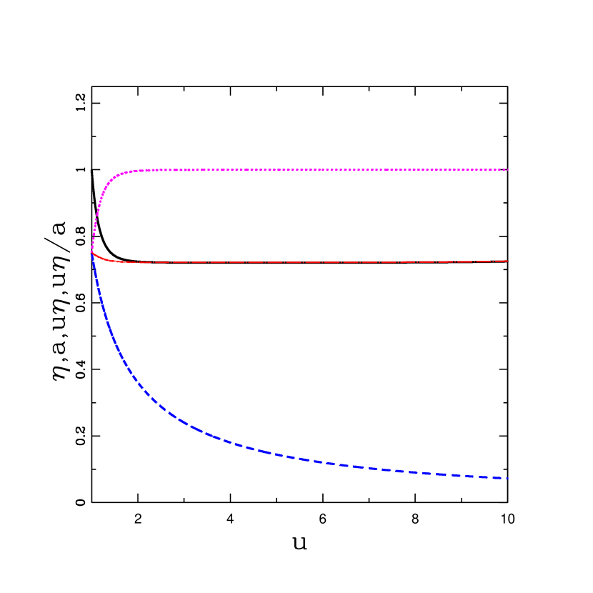
Figure 1: Field variables as a function of $u=1/m(t)$ for typical system with $\beta=2$, $q=7$, $\eta_{0}=0.75$, and $p=0$. The plot shows the semimajor axis (black solid curve), angular momentum parameter $\eta$ (blue dashed curve), the product $u\eta$ (red dot-dashed curve), and the combination $u\eta/a$ (magenta dotted curve).

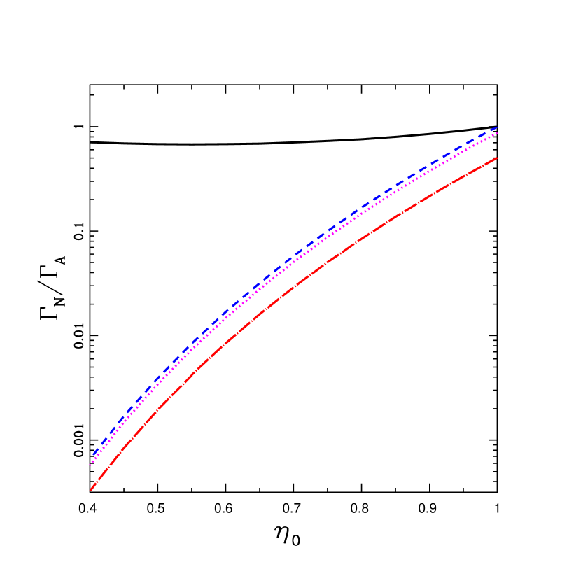
Figure 2: Critical value of tidal dissipation parameter $\Gamma$ that marks the boundary between planetary accretion and survival. Results are shown for three cases with $q=7$ and varying indices $(\beta,p)$. Solid black curve shows the ratio $\Gamma_{N}/\Gamma_{A}$ versus starting angular momentum parameter $\eta_{0}$ (same for all models). For comparison, the analytic estimate itself $\Gamma_{A}/\gamma=\eta_{0}^{q+1}(q+\beta-p-1)/(q+1)$ is plotted for indices ($\beta=2,p=0$; blue dashed curve), ($\beta=1,p=0$; magenta dotted curve), and ($\beta=2,p=4$; red dot-dashed curve).

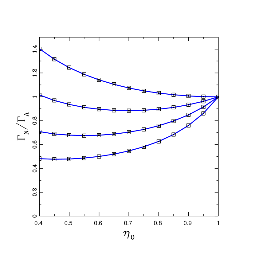
Figure 3: Critical value of tidal dissipation parameter ($\Gamma_{N}/\Gamma_{A}$) for different indices $q=5-8$ (from top to bottom), plotted versus starting angular momentum parameter $\eta_{0}$. All cases use $p=0$. Solid curves (blue) show results for $\beta=2$, whereas symbols show results for $\beta=1$ (smaller squares) and $\beta=3$ (larger squares); the results are essentially independent of $\beta$.

3 Numerical Results

Equation (25) provides an analytic estimate for the value of $\Gamma$ the marks the boundary between systems where planets are accreted and those where they survive. We denote this analytic value as $\Gamma_{A}$. In this section we numerically integrate the equations of motion to determine the value $\Gamma_{N}$ that marks this boundary. As shown below, the analytic estimates are quite good, in that the ratio $\Gamma_{N}/\Gamma_{A}$ is always of order unity.

Individual orbits are integrated using a Bulirsch-Stoer alogrithm, where the relative error per time step is $10^{-12}$; in the iteration loop for the critical value of $\Gamma$, the relative error due to lack of convergence is $\approx 3\times 10^{-5}$. Numerical errors are thus negligible.

Figure 1 shows how the system variables evolve with time for a typical model ($\beta=2,q=7,p=0,\eta_{0}=0.75$). The angular momentum parameter $\eta$ steadily decreases with time, whereas the semimajor axis $a$ and the product $u\eta$ approach constant values. The combination $u\eta/a$ approaches unity. This type of evolution occurs over a wide range of the parameter space (not shown).

Figures 2 and 3 show the ratio $\Gamma_{N}/\Gamma_{A}$ as a function of the starting value of the angular momentum parameter $\eta_{0}$. These calculations use $\gamma=10^{-4}$; the results are indpendent of $\gamma$ provided that $\gamma\ll 1$. Figure 2 also shows the right-hand-side of equation (25). Note that for $\eta_{0}<1$, this quantity decreases rapidly, varying by several orders of magnitude for the cases shown here. Although the $\Gamma_{N}$ value that marks the boundary varies by several orders of magnitude, the ratio $\Gamma_{N}/\Gamma_{A}$ always remains of order unity.

Our numerical exploration reveals the following general results: [1] For circular orbits with $\eta_{0}=1$, the ratio $\Gamma_{N}/\Gamma_{A}=1$, so that the analytic estimate from equation (25) is exact. [2] The numerically-determined results for $\Gamma_{N}/\Gamma_{A}$ are independent of the mass loss index $\beta$ (where we focus on the range $\beta=1-3$). Similarly, the results for $\Gamma_{N}/\Gamma_{A}$ are independent of the index $p$ that determines how tidal dissipation depends on changing stellar radius during the mass loss epoch. [3] All of the results shown here are carried out for orbits that start at periastron and for small $\gamma=10^{-4}$. Our numerical work shows that the results are independent of the starting orbital phase $\theta$ for sufficiently small $\gamma$, but order-unity differences arise for larger $\gamma\,\raise 1.29167pt\hbox{$>$}\kern-7.5pt\lower 3.01385pt\hbox{$\sim$}\,0.001$. However, stellar mass loss takes place over $0.1-1$ Myr, and planets near the border have $a\approx 1$ AU, so the physically-relevant values lie in the range $\gamma=10^{-6}-10^{-4}$. [4] The ratio $\Gamma_{N}/\Gamma_{A}$ depends weakly on the index $q$ that determines how tidal dissipation depends on radial distance. Figure 3 illustrates this behavior by plotting the ratio $\Gamma_{N}/\Gamma_{A}$ versus the starting angular momentum parameter $\eta_{0}$ for $q=5-8$. Although the critical value of $\Gamma$ itself varies by several orders of magnitude over the parameter space depicted by the figure, the ratio $\Gamma_{N}/\Gamma_{A}$ remains of order unity for all $q$ (and is independent of $\beta$ and $p$).

4 Effects of Radial Pulsation

This section revisits the leading order solution with the inclusion of non-monotonic variations in the stellar radius. The radial pulsations of the star often appear to be periodic, or nearly periodic (Vassiliadis & Wood, 1993). Since the tidal dissipation term is proportional to the stellar radius to a high power, even small changes can make a difference. To incorporate the radial variations, we multiply the tidal dissipation term by a factor of the form

$${F}=1+bQ(t),$$ (27)

where $Q(t)$ is a quasi-periodic function with vanishing mean and where the parameter $b$ is determined by the pulsation amplitude. To leading order, the equations of motion have the form

$${\gamma}u^{\beta-p}{d\eta\over{du}}=-\Gamma\xi^{-q}\left[1+bQ(u)\right]\qquad{\rm and}\qquad\xi=u\eta+{\cal O}(\gamma^{2}),$$ (28)

where the time dependence of the quasi-periodic function $Q$ is written in terms of $u$. After eliminating $\xi$, as before, we integrate to find the solution $\eta(u)$,

$$\eta^{q+1}=\eta_{0}^{q+1}-{(q+1)\over(q+\beta-p-1)}{\Gamma\over\gamma}\left[1-u^{-(q+\beta-p-1)}\right]-{b(q+1)\Gamma\over\gamma}\int_{1}^{u}{u^{-(q+\beta-p)}}Q(u)du.$$ (29)

It is convenient to define the integral quantity

$${I}(u)\equiv\int_{1}^{u}{u^{-(q+\beta-p)}}Q(u)du.$$ (30)

Converting back to the function $\xi$, we have the solution

$$\xi^{q+1}=u^{q+1}\left[\eta_{0}^{q+1}-{(q+1)\over(q+\beta-p-1)}{\Gamma\over\gamma}\right]+{(q+1)\over(q+\beta-p-1)}{\Gamma\over\gamma}u^{2-\beta+p}-{b(q+1)\Gamma\over\gamma}u^{q+1}I(u).$$ (31)

The indices generally obey the ordering $q+1>2-\beta+p$, and we expect the integral $I$ to converge. At late times, corresponding to large $u$, we want the solution $\eta(u)$ to approach zero and the solution $\xi(u)$ to remain finite. These conditions imply that the critical value of the tidal dissipation parameter is given by

$${\Gamma\over\gamma}=\eta_{0}^{q+1}{(q+\beta-p-1)\over(q+1)}\left[1+b(q+\beta-p-1)I_{\infty}\right]^{-1},$$ (32)

where we take the limit $u\to\infty$ to evalute the integral. The quantity $I_{\infty}$ is usually, but not always, positive. As a result, the effect of radial pulsations is (usually) to reduce the size of the tidal dissipation parameter needed to make planets spiral inward and be accreted by the star. In other words, pulsations generally result in more tidal dissipation, compared to the average (recall that $Q(t)$ has zero mean by definition).

To illustrate the effects of pulsations, we consider the tidal dissipation strength to vary with time as a sine function, i.e.,

$${Q}(t)=\sin\omega{t},$$ (33)

where the pulsation period $P=2\pi/\omega$. For exponential mass loss ($\beta=1$), $p=0$, and arbitrary $q$, we must evaluate the integral

$${I_{\infty}}=\int_{1}^{\infty}{u^{-(q+\beta)}}Q(u)du=\int_{1}^{\infty}{du}u^{-(q+1)}\sin\left[{\omega\over\gamma}\ln{u}\right],$$ (34)

which reduces to the form

$${I_{\infty}}={\gamma\omega\over\omega^{2}+q^{2}\gamma^{2}}.$$ (35)

As another example, consider the $Q(t)$ profile from equation (33) with constant mass loss rate ($\beta=2$) and index $q=8$; the integral $I_{\infty}$ then becomes

$${I_{\infty}}={40320(1-\cos[\omega/\gamma])-20160(\omega/\gamma)^{2}+1680(\omega/\gamma)^{4}-56(\omega/\gamma)^{6}+(\omega/\gamma)^{8}\over(\omega/\gamma)^{9}}.$$ (36)

Equations (35,36) represent two typical cases; one can evaluate $I_{\infty}$ for any pulse profile and choice of indices (although the integral sometimes must be done numerically, and we require $q+\beta>p+1$ for convergence).

These results depend on $\omega/\gamma$, which typically falls in the range $\omega/\gamma\approx 50-150$ for post-main-sequence stars during their mass-loss epoch (Vassiliadis & Wood, 1993). In the limit where the pulse frequency is large compared to the mass loss rate, $\omega\gg\gamma$, the integral $I_{\infty}\to 0$, as expected: In this limit, oscillations of the stellar radius average to zero. For pulsations to produce an appreciable effect, the system must experience non-trivial evolution (mass loss) during the course of a pulse (to break the symmetry). Notice also that $I_{\infty}\to 0$ as $\omega\to 0$, the limit where pulsations effectively vanish.

With the integral $I_{\infty}$ specified, the critical tidal damping parameter is given by equation (32). For initially circular orbits, this result is exact: Figure 4 shows the numerically-determined value of the critical tidal damping parameter for stars experiencing pulsations specified by equation (33), plotted versus frequency $\omega/\gamma$. The upper curves correspond to initially circular orbits ($\eta_{0}=1$), with $\beta=1$ (solid-green) and $\beta=2$ (dot-dashed-blue). The square symbols show the analytically predicted results from equation (32), using equations (35) and (36), respectively. The lower curves show results for $\eta_{0}=0.9$ (red) and 0.8 (cyan). Here, the square symbols represent the numerical result with no pulsations (see Figure 3) scaled using the pulsation correction factor $[1+b(q+\beta-p-1)I_{\infty}]$.

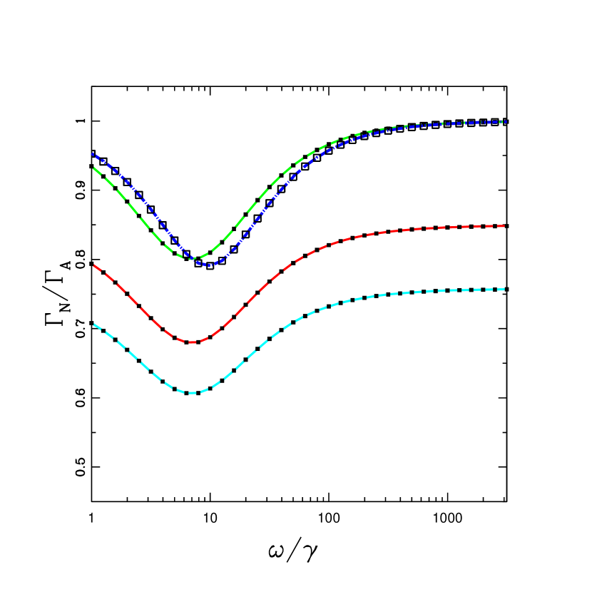
Figure 4: Critical tidal dissipation parameter ($\Gamma_{N}/\Gamma_{A}$), the boundary between planetary accretion and survival, plotted versus pulsation frequency $\omega/\gamma$, for systems undergoing sinusoidal pulsations (with amplitude $b=0.5$). Solid curves show numerically-determined results (for $\beta=1,q=7,p=0$), for initial angular momentum $\eta_{0}=1$ (top green), 0.9 (middle red), and 0.8 (bottom cyan); solid squares show the corresponding analytic predictions. Dot-dashed (blue) curve shows the critical $\Gamma$ for constant mass loss rate $\beta=2$ (and $q=8$).

5 Conclusion

Motivated by observations indicating that planets often orbit both intermediate mass stars and stellar remnants, this paper considers the combined effects of stellar mass loss and tidal dissipation on planetary orbits. Mass loss allows planetary orbits to spiral outward, whereas tidal dissipation acts to move planets inward. This work determines the critical value of the tidal dissipation parameter that marks the boundary between these two fates. To address this question, we have developed a parametric model for orbital evolution that accounts for stellar mass loss (equations [4, 17]) and dissipation (equation [6]). These effects are specified by dimensionless rates ($\gamma,\Gamma$), and indices that determine their functional forms ($\beta,q,p$). The initial conditions are specified by the starting angular momentum $\eta_{0}$ and orbital phase $\theta$ (although the results are independent of $\theta$ for $\gamma\ll 1$).

The main result of this work is an analytic expression for the critical tidal dissipation rate $\Gamma$ that determines the boundary between planetary survival and accretion (equation [25]). This formula specifies the dependence of the critical $\Gamma$ on starting angular momentum $\eta_{0}$, mass loss rate $\gamma$, mass loss index $\beta$, dissipation radial index $q$, and dissipation mass index $p$ (see equation [25]). The resulting expression is accurate to $\approx 50\%$ over entire 7-dimensional parameter space $(\Gamma,\gamma,\beta,q,p,\eta_{0},\theta)$, even though individual parameters vary over several orders of magnitude (see Figures 2 and 3); moreover, the analytic result is effectively exact for initially circular orbits. These results show that the most important variable in the problem is the ratio $\Gamma/\gamma$, which can be written in scaled form,

$${\Gamma\over\gamma}\approx\left({\tau\over 0.1{\rm Myr}}\right)\left({M_{P}\over{M_{J}}}\right)\left({M_{\ast 0}\over 1M_{\odot}}\right)^{-1/2}\left({R_{\ast 0}\over 1{\rm AU}}\right)^{8}\left({a_{0}\over 2{\rm AU}}\right)^{-19/2},$$ (37)

where the timescale $\tau=M_{\ast 0}/\dot{M}_{\ast 0}$. Combining this expression with the critical tidal dissipation parameter (equation [25]), we find the innermost orbits where planets survive,

$$\left({a_{0}\over 2{\rm AU}}\right)\approx\eta_{0}^{2(q+1)/19}\left[{q+1\over{q+\beta-p-1}}\left({\tau\over 0.1{\rm Myr}}\right)\left({M_{P}\over{M_{J}}}\right)\right]^{2/19}\left({M_{\ast 0}\over 1M_{\odot}}\right)^{-1/19}\left({R_{\ast 0}\over 1{\rm AU}}\right)^{16/19}.$$ (38)

This work includes an important additional complication: evolved stars often display pulsating variations in stellar radius, which produce corresponding variations in tidal dissipation. Section 4 includes stellar pulsations in the formulation and estimates the generalized critical value of the tidal dissipation parameter (equation [32]); this semi-analytic expression holds to the same accuracy as the non-pulsating case (Figure 4).

Previous studies of planetary orbits with stellar mass loss indicate that the product of mass and semimajor axis often remains nearly constant, and this approximation ($am=constant$) is often used (Veras et al. 2011; Mustill & Villaver 2012). For purposes of finding the critical tidal dissipation strength, however, this approximation breaks down: The orbits of interest arise near the boundaries of parameter space, where the planets are close to spiraling inward. But if a planet spirals inward as the star loses mass, the product $am$ would decrease ($am\neq{constant}$). A more applicable approximation (correct to leading order) is the generalized law

$${\xi{m}\over\eta}\approx{constant},$$ (39)

where $\eta$ decreases with time. For orbits that spiral outward, tidal dissipation quickly becomes negligible, so that the angular momentum parameter $\eta$ becomes nearly constant; in this case, one recovers the old result ($am\approx\xi{m}\approx{constant}$).

The analytic expressions for the critical dissipation strength $\Gamma$, given by equations (25) and (32), are accurate for the physically-relevant portion of parameter space. Nonetheless, these results must be used within their domain of applicability. The approximations used herein break down when the dimensionless mass loss rate becomes large ($\gamma\gg 0.001$) and/or for index combinations satisfying $q+\beta\leq{p+1}$. This treatment only considers the dissipation of the equilibrium tide in the convective envelope of the star; future work should also include tidal dissipation within the planet (although it is smaller and more uncertain).

Acknowledgments: We thank D. Veras for useful comments. This work was supported by NSF Grants DMS097949 and DMS1207693.

References

- Adams et al. (2013) Adams, F. C., Anderson, K. R., & Bloch, A. M. 2013, MNRAS, 432, 438 (AAB2013)
- Debes & Sigurdsson (2002) Debes, J. H., & Sigurdsson, S. 2002, ApJ, 572, 556
- Farihi et al. (2009) Farihi, J., Jura, M., & Zuckerman, B. 2009, ApJ, 694, 805
- Farihi et al. (2010) Farihi, J., Jura, M., Lee, J.-E., & Zuckerman, B. 2010, ApJ, 714, 1386
- Gänsicke et al. (2006) Gänsicke, B. T., Marsh, T. R., Southworth, J., & Rebassa-Mansergas, A. 2006, Science, 314, 1908
- Gänsicke et al. (2007) Gänsicke, B. T., Marsh, T. R., & Southworth, J. 2007, MNRAS, 380, 35
- Gettel et al. (2012) Gettel, S., Wolszczan, A., Niedzielski, A., Nowak, G., Adamów, M., Zieliński, P., & Maciejewski, G. 2012, ApJ, 745, 28
- Hadjidemetriou (1963) Hadjidemetriou, J. D. 1963, Icarus, 2, 440
- Hadjidemetriou (1966) Hadjidemetriou, J. D. 1966, Icarus, 5, 34
- Hurley et al. (2000) Hurley, J. R., Pols, O. R., & Tout, C. A. 2000, MNRAS, 315, 543
- Hut (1981) Hut, P. 1981, A&A, 99, 126
- Jeans (1924) Jeans, J. H. 1924, MNRAS, 85, 2
- Jura (2003) Jura, M., 2003, ApJ, 584, L91
- Jura et al. (2007) Jura, M., Farihi, J., & Zuckerman, B. 2007, ApJ, 663, 1285
- Kunitomo et al. (2011) Kunitomo, M., Ikoma, M., Sato, B., Katsuta, Y., & Ida, S. 2011, ApJ, 737, 66
- Melis et al. (2010) Melis, C., Jura, M., Albert, L., Klein, B., & Zuckerman, B. 2010, ApJ, 722, 1078
- Mustill & Villaver (2012) Mustill, A. J., & Villaver, E. 2012, ApJ, 761, 121
- Nordhaus et al. (2010) Nordhaus, J., Spiegel, D. S., Ibgui, L., Goodman, J., & Burrows, A. 2010, MNRAS, 408, 631
- Nordhaus & Spiegel (2013) Nordhaus, J., & Spiegel, D. S. 2013, MNRAS, 432, 500
- Schröder & Connon Smith (2008) Schröder, K.-P., & Connon Smith, R. 2008, MNRAS, 386, 155
- Spiegel & Madhusudhan (2012) Spiegel, D. S., & Madhusudhan, N. 2012, ApJ, 756, 132
- Vassiliadis & Wood (1993) Vassiliadis, E., & Wood, P. R. 1993, ApJ, 413, 641
- Veras et al. (2011) Veras, D., Wyatt, M. C., Mustill, A. J., Bonsor, A., & Eldridge, J. J. 2011, MNRAS, 417, 2104
- Veras & Tout (2012) Veras, D., & Tout, C. A. 2012, MNRAS, 422, 1648
- Verbunt & Phinney (1995) Verbunt, F., & Phinney, E. S. 1995, A&A, 296, 709
- Villaver & Livio (2007) Villaver, E., & Livio, M. 2007, ApJ, 661, 1192
- Villaver & Livio (2009) Villaver, E., & Livio, M. 2009, ApJ, 705, 81
- Wolszczan (1994) Wolszczan, A. 1994, Science, 264, 538
- Zahn (1977) Zahn, J.-P. 1977, A&A, 57, 383
- Zuckerman et al. (2003) Zuckerman, B., Koester, D., Reid, I. N., & Hünsch, M. 2003, ApJ, 596, 477
- Zuckerman et al. (2010) Zuckerman, B., Melis, C., Klein, B., Koester, D., & Jura, M. 2010, ApJ, 722, 725