Local observers on linear Lie groups with linear estimation error dynamics

Abstract

This paper proposes local exponential observers for systems on linear Lie groups. We study two different classes of systems. In the first class, the full state of the system evolves on a linear Lie group and is available for measurement. In the second class, only part of the system’s state evolves on a linear Lie group and this portion of the state is available for measurement. In each case, we propose two different observer designs. We show that, depending on the observer chosen, local exponential stability of one of the two observation error dynamics, left or right invariant error dynamics, is obtained. For the first class of systems these results are developed by showing that the estimation error dynamics are differentially equivalent to a stable linear differential equation on a vector space. For the second class of system, the estimation error dynamics are almost linear. We illustrate these observer designs on an attitude estimation problem.

1 Introduction

Observers for systems on Lie groups is an active area of research [1]. Interest in this research has been partially motivated by the problem of controlling mobile robots, and in particular, unmanned aerial vehicles (UAVs). Precise control of these systems requires accurate estimates of the orientation of a rigid-body using low cost on-board sensors  [2]. Small autonomous robots usually undergo significant vibration and other disturbances, while being restricted to carrying only a basic light-weight sensor package. For this reason, high-frequency noise is often present in the sensor measurements of these robots. Nonlinear observers for systems on Lie groups are useful because, in certain cases, they can be used to filter out the sensor noise.

Recent work on full-state observers for systems on $\mathsf{SO}\left(3,\mathbb{R}\right)$, describing rigid-body rotational kinematics, was done in [3],  [4]. The algorithms in  [3],  [4] rely on a projection of the measurement error from the Lie group to its Lie algebra. The projected vector in the Lie algebra is then used to drive the observer to converge to the system trajectory. While this projection based approach does not work for systems on the general linear Lie group, $\mathsf{GL}\left(n,\mathbb{R}\right)$, the work in [5] may contain ideas to extend these projection based observers to the general linear group.

For systems on $\mathsf{SO}\left(3\right)$ with partial state measurements, the paper [6] proposes an observer that uses measurements of the orientation and of the torque to estimate the angular velocity of the rigid-body. The papers  [7],  [8] propose globally exponentially convergent observers using partial state measurements. The work in  [9] also uses partial state measurements in their observers. The paper [10] analyses the effect of noise on an attitude estimation observer. The authors of [11] propose observers for $\mathsf{SO}\left(n,\mathbb{R}\right)$.

For systems on $\mathsf{SE}\left(3,\mathbb{R}\right)$, describing rigid-body pose, full-state observers were proposed in  [12],  [13],  [14]. For systems on $\mathsf{SL}\left(3,\mathbb{R}\right)$, describing a homography transformation, partial-state observers were proposed in [15].

In this paper, we consider left-invariant systems on the general linear Lie group, i.e., the group of all invertible, real $n\times n$ matrices. The output of the system is taken to be that portion of the state evolving on the linear Lie group. We first consider the case in which the entire state evolves on the Lie group. We call these Lie group full-state observers. Then we consider the case where the states evolving on the Lie group are only a subset of the systems entire state. We call these Lie group partial-state observers.

A recent breakthrough in observer design on the general linear Lie group was achieved in [16], where exponentially converging observers are proposed for left-invariant and right-invariant systems on arbitrary finite dimensional, connected Lie groups. The proposed exponential observer uses gradient-like driving terms, derived from cost functions of the Lie group measurement error. In this paper we propose an alternative to gradient-like observers. Our observers are noteworthy because they yield linear estimation error dynamics. A weakness of our result is that we only prove local exponential stability.

A vector field on a connected Lie group is said to be linear if its flow is a one-parameter subgroup [17]. Recent work on linear vector fields and linear systems on Lie groups was done in [17] and [18]. The estimation error dynamics of our Lie group full-state observers are shown to be linear vector fields on the Lie group. We also show that the estimation error dynamics are differentially equivalent, by means of the logarithm map, to a linear vector field on the Lie algebra.

The research in [19], [20] considers a more general class of systems than the left-invariant systems considered in this paper. These articles consider systems that evolve on a vector space, but are such that a certain Lie group action leaves the system equations unchanged. This shows that, if the plant is invariant under the action of some Lie group, then part of the states of the plant can be redefined as evolving on this Lie group, at least locally.

The main contributions of this paper include the exponential full-state observer in Section 5.1 for left-invariant systems on the general linear Lie group. Our observer yields linear estimation error dynamics, distinguishing it from other observers in the literature. In Section 5.1 we propose an exponential partial-state observer, for a class of systems that is a generalization of the left-invariant systems considered in  5.1. This class of systems has only a proper subset of its states evolving on the Lie group, while the rest of the states evolve on the Lie algebra. The results in Section 7 show equivalence properties for certain differential equations on $\mathsf{GL}\left(n,\mathbb{R}\right)$. The effectiveness of the proposed observers is illustrated via simulation in Section 9.

2 Motivation

Attitude control of a rigid body, like a UAV, is simplified if accurate estimates of its orientation are available. The attitude of a rigid body in Euclidean three-dimensional space is specified by the relative orientation between a coordinate frame fixed to the body and an inertial coordinate system. The orientation between the frames is described by means of a rotation matrix. If we denote the body frame by $\mathcal{F}_{b}$ and the inertial frame by $\mathcal{F}_{a}$ then the rotation matrix $R_{ab}$ relating $\mathcal{F}_{b}$ to $\mathcal{F}_{a}$ is an element of the special orthogonal group $\mathsf{SO}\left(3,\mathbb{R}\right)\subset\mathbb{R}^{3\times 3}$.

If we assume that the orientation of the body frame $\mathcal{F}_{b}$ with respect to the inertial frame $\mathcal{F}_{a}$ varies in time, then the entries of $R_{ab}$ become functions of time. By differentiating the identities $R_{ab}R^{\top}_{ab}=I$ and $R^{\top}_{ab}R_{ab}=I$ one can show that $\dot{R}_{ab}R^{\top}_{ab}$ and $R^{\top}_{ab}\dot{R}_{ab}$ are skew-symmetric. Define $\operatorname{Skew}{(\omega^{a}_{ab})}\coloneqq\dot{R}_{ab}R^{\top}_{ab}$ where $\operatorname{Skew}:\mathbb{R}^{3}\to\mathbb{R}^{3\times 3}$ takes any vector in $v=\operatorname{col}(v_{1},v_{2},v_{3})\in\mathbb{R}^{3}$ and maps it to a skew-symmetric matrix

$$\operatorname{Skew}{(v)}=\left[\begin{array}[]{ccc}0&-v_{3}&v_{2}\\ v_{3}&0&-v_{1}\\ -v_{2}&v_{1}&0\end{array}\right].$$

The vector $\omega^{a}_{ab}$ is called the instantaneous inertial angular velocity. It represents the instantaneous angular velocity of the rigid body as seen from $\mathcal{F}_{a}$. Similarly, define the instantaneous body angular velocity $\omega^{b}_{ab}$ via $\operatorname{Skew}{(\omega^{b}_{ab})}\coloneqq R^{\top}_{ab}\dot{R}_{ab}$. The matrix $R_{ab}(t)$ is therefore the solution of either of the differential equations

$$\dot{R}_{ab}=R_{ab}\operatorname{Skew}{(\omega^{a}_{ab})},\qquad\dot{R}_{ab}=\operatorname{Skew}{(\omega^{b}_{ab})}R_{ab}.$$

These equations are kinematic since they do not involve forces or torques. In this paper we consider a class of systems that includes the first of these two differential equations, i.e., we consider kinematic systems of the form

$$\dot{R} =Ru$$ (1)

$$Y =R,$$

where $Y\in\mathsf{SO}\left(3,\mathbb{R}\right)$ is a direct measurement of $R$. This equation is relevant to attitude control problems because $Y$ and $u$ can be measured or estimated using low-cost sensors, mounted on the body frame $\mathcal{F}_{b}$. In fact, $u$ can be measured using angular rate gyroscopes, while the rotation matrix $Y$ can be calculated from sensor measurements, made by an accelerometer and magnetometer pair.

Given these measurements, in Section 5 we design an observer to estimate the state of (1). Our observer enjoys the property that if the estimate of $R$ isn’t too erroneous initially, then the estimate will converge to $R$ exponentially and the rate of convergence can be easily tuned using a single parameter. At first glance it may seem unnecessary to design an observer to estimate the state of a system if that state is already measured. We are motivated to study this problem for two reasons. First such an observer provides noise filtering and can be used as a sensor fusion algorithm [3],  [4]. The second reason is that by looking at this simple case we hope to gain insight into the state estimation problem when the output is not equal to the entire state.

In the latter case, consider a dynamic model of (1)

$$\dot{R} =R\omega$$ (2)

$$\dot{\omega} =u$$

$$Y =R$$

where $\omega$ and $u$ are skew-symmetric matrices. Here $Y=R$ is directly measured as well as the angular acceleration $u$. In Section 5 we propose observers that fuse these two sensor measurements to obtain an estimate of angular velocity, $\omega$, and also to filter out noise from $Y$.

3 Notation and Preliminaries

We denote by $\mathbb{R}^{+}$ the set of real numbers, equipped with the additive group structure. Let $\mathbb{R}_{\leq 0}\coloneqq(-\infty,0]$. The empty set is $\varnothing$. If $z\in\mathbb{C}$, then $\operatorname{Re}{(z)}$ and $\operatorname{Im}{(z)}$ denote its real and imaginary parts. We denote by $\mathbb{R}^{n\times n}$ the set of $n\times n$ matrices with real entries. If $X\in\mathbb{R}^{n\times n}$ then $\sigma(X)$ denotes the eigenvalues of $X$. If $x\in\mathbb{R}^{n}$, then $x_{i}$ refers to the $i$th component of $x$. If $X\in\mathbb{R}^{n\times n}$, then $X_{ij}$ refers to the $(i,j)$th element of $X$. The symbols $I_{n}$ and $0_{n}$ denote the $n\times n$ identity matrix and $n\times n$ zero matrix respectively. If $A\in\mathbb{R}^{n\times n}$ then $A^{\top}$ denotes the transpose of $A$ and $\operatorname{trace}(A)$ denotes its trace, i.e., $\operatorname{trace}{(A)}=\sum^{n}_{i}A_{ii}$.

We denote by $\mathsf{GL}\left(n,\mathbb{R}\right)$ the general linear Lie group of all invertible $n\times n$ matrices with real entries and matrix multiplication as the group operation

$$\mathsf{GL}\left(n,\mathbb{R}\right) \coloneqq\{X\in\mathbb{R}^{n\times n}:\det(X)\neq 0\}.$$

We denote by $\mathsf{M}\left(n,\mathbb{R}\right)$ the algebra of all $n\times n$ matrices with real entries. The bilinear product that makes $\mathsf{M}\left(n,\mathbb{R}\right)$ an algebra is the matrix commutator, i.e., given $A,B\in\mathsf{M}\left(n,\mathbb{R}\right)$, the product of $A$ and $B$ is $[A,B]\coloneqq AB-BA$. For matrices $A\in\mathsf{M}\left(n,\mathbb{R}\right)$ and $X\in\mathsf{GL}\left(n,\mathbb{R}\right)$, the adjoint map is $\operatorname{Ad}_{X}(A)\coloneqq XAX^{-1}$.

For a vector $x\in\mathbb{R}^{n}$, $\|x\|$ denotes the Euclidean norm. For a matrix $A\in\mathbb{R}^{n\times n}$, the induced matrix norm is

$$\|A\|\coloneqq\max\left\{\|Ax\|:x\in\mathbb{R}^{n},\|x\|\leq 1\right\}.$$

Induced norms on $\mathbb{R}^{n\times n}$ are submultiplicative [21], i.e., for any $A$, $B\in\mathbb{R}^{n\times n}$, $\|AB\|\leq\|A\|\|B\|$. Given a matrix $A\in\mathbb{R}^{n\times n}$ and a real scalar $r>0$, define the open ball

$$B(A,r)\coloneqq\left\{X\in\mathbb{R}^{n\times n}:\|A-X\|<r\right\}.$$ (3)

Proposition 3.1.

Let $X\in B(I_{n},1)$, then the series $\sum_{k=0}^{\infty}(-1)^{k}(X-I_{n})^{k}$ converges in norm and

$$X^{-1}=\sum_{k=0}^{\infty}(-1)^{k}(X-I_{n})^{k}.$$ (4)

Proof.

Let $X\in B(I_{n},1)$ and define $M\coloneqq I_{n}-X$ so that $\|M\|<1$. Taking the norm of the right hand side of (4)

$$\left\|\sum_{k=0}^{\infty}(-1)^{k}(X-I_{n})^{k}\right\| =\left\|\sum_{k=0}^{\infty}M^{k}\right\|$$

$$\leq\sum_{k=0}^{\infty}\|M^{k}\|$$

$$\leq\sum_{k=0}^{\infty}\|M\|^{k}$$

$$=(1-||M||)^{-1}.$$

Hence the right hand side of (4) is a convergent series. To see that its sum equals $X^{-1}$, since $X$ is a square matrix, it is enough to left-multiply by $X$ and to check that the result is the identity matrix. To this end

$$X\sum_{k=0}^{\infty}(-1)^{k}(X-I_{n})^{k} =(I_{n}-M)\sum_{k=0}^{\infty}M^{k}$$

$$=\sum_{k=0}^{\infty}\left(M^{k}-M^{k+1}\right)$$

$$=I_{n}+\sum_{k=1}^{\infty}\left(M^{k}\right)-\sum_{k=0}^{\infty}\left(M^{k+1}\right)$$

$$=I_{n}+M-M+M^{2}-M^{2}+\cdots$$

$$=I_{n}.$$

∎

A consequence of Proposition 3.1 is that the set $B(I_{n},1)$ is contained in $\mathsf{GL}\left(n,\mathbb{R}\right)$.

3.1 Linear Lie groups

In this section, we give a brief introduction to Lie groups as subgroups of matrices. The main mathematical references are [22], [23]. All the results in this section are standard.

Definition 3.2.

A linear Lie group $\mathsf{G}$ is a closed subgroup of $\mathsf{GL}\left(n,\mathbb{R}\right)$.

A linear Lie group is not the same thing as a matrix Lie group. A matrix Lie group is a subgroup of $\mathsf{GL}\left(n,\mathbb{R}\right)$ ([24, Definition 5.13]), but not necessarily closed as a set. For example the subgroup $\mathsf{GL}\left(n,\mathbb{Q}\right)$ of rational matrices with rational inverses is not closed in the topology of $\mathbb{R}^{n\times n}$. The fact that linear groups are additionally restricted to be closed sets ensures, by the Closed Subgroup Theorem [25, Theorem 20.10], that the Lie group is an embedded submanifold of $\mathbb{R}^{n\times n}$. Working with Lie groups that are embedded submanifolds of $\mathbb{R}^{n\times n}$, rather than abstract manifolds, allows us to perform computations in the embedding space. In particular, this permits the use of standard vector calculus. The idea of doing computations in a larger and simpler embedding manifold is one of the key ideas in [5], see also [26]. For brevity, the term Lie group is used in place of linear Lie group throughout. In addition to $\mathsf{GL}\left(n,\mathbb{R}\right)$, the following linear Lie groups are used in this paper

$$\mathsf{SL}\left(n,\mathbb{R}\right) \coloneqq\{X\in\mathbb{R}^{n\times n}:\det(X)=1\},$$

$$\mathsf{SO}\left(n,\mathbb{R}\right) \coloneqq\{X\in\mathbb{R}^{n\times n}:XX^{\top}=I_{n},\det(X)=1\}.$$

Definition 3.3.

Given a matrix $A\in\mathsf{M}\left(n,\mathbb{R}\right)$, the matrix exponential $\exp:\mathsf{M}\left(n,\mathbb{R}\right)\rightarrow\mathsf{GL}\left(n,\mathbb{R}\right)$ is defined to be

$$\exp(A)\coloneqq\sum_{k=0}^{\infty}\frac{A^{k}}{k!}.$$ (5)

Since $\|A^{k}\|\leq\|A\|^{k}$, the series (5) converges in norm for every matrix $A\in\mathbb{R}^{n\times n}$.

Definition 3.4.

Given a linear Lie group $\mathsf{G}$, the Lie algebra of $\mathsf{G}$, denoted by $\operatorname{Lie}(\mathsf{G})$, is the set

$$\operatorname{Lie}(\mathsf{G})\coloneqq\left\{A\in\mathsf{M}\left(n,\mathbb{R}\right):\;\left(\forall\;t\in\mathbb{R}\right)\exp(tA)\in\mathsf{G}\right\}.$$

The results [22, Theorem 3.2.1], [24, Theorem 5.20] show that $\operatorname{Lie}(\mathsf{G})$ is a subalgebra of $\mathsf{M}\left(n,\mathbb{R}\right)$. The Lie algebras encountered in this paper are given by

$$\operatorname{Lie}(\mathsf{GL}\left(n,\mathbb{R}\right))\coloneqq\mathsf{M}\left(n,\mathbb{R}\right)$$

$$\operatorname{Lie}(\mathsf{SL}\left(n,\mathbb{R}\right))\coloneqq\{A\in\mathsf{M}\left(n,\mathbb{R}\right):\operatorname{trace}(A)=0\}$$

$$\operatorname{Lie}(\mathsf{SO}\left(n,\mathbb{R}\right))\coloneqq\{A\in\mathsf{M}\left(n,\mathbb{R}\right):A+A^{\top}=0_{n}\}.$$

Definition 3.5.

Let $\mathsf{G}$ be a linear Lie group. A one-parameter subgroup of $\mathsf{G}$ is a continuous group homomorphism $\gamma:\mathbb{R}^{+}\rightarrow\mathsf{G}$.

Lemma 3.6 ([22, Theorem 3.1.1]).

If $\gamma:\mathbb{R}^{+}\rightarrow\mathsf{GL}\left(n,\mathbb{R}\right)$ is a one-parameter subgroup of $\mathsf{GL}\left(n,\mathbb{R}\right)$, then $\gamma$ is real-analytic and $\gamma(t)=\exp(tA)$, with $A=\gamma^{\prime}(0)$.

Lemma 3.7.

Let $X:\mathbb{R}\rightarrow\mathsf{GL}\left(n,\mathbb{R}\right)$ be a smooth parameterized curve. Then

$$\frac{\mathrm{d}}{\mathrm{d}\tau}X^{-1} =-X^{-1}\frac{\mathrm{d}X}{\mathrm{d}\tau}X^{-1}.$$ (6)

Proof.

For any smooth parameterized curve $X:\mathbb{R}\rightarrow\mathsf{GL}\left(n,\mathbb{R}\right)$, and any $\tau\in\mathbb{R}$, $X(\tau)X^{-1}(\tau)=I_{n}$ where $\tau$ is the curve parameter. Differentiating both sides of this identity with respect to $\tau$, while using the product rule, we get

$$0=\frac{\mathrm{d}}{\mathrm{d}\tau}I_{n} =\frac{\mathrm{d}}{\mathrm{d}\tau}\left(XX^{-1}\right)$$

$$=\frac{\mathrm{d}X}{\mathrm{d}\tau}X^{-1}+X\frac{\mathrm{d}X^{-1}}{\mathrm{d}\tau},$$

from which (6) immediately follows. ∎

Definition 3.8.

Given a smooth parameterized curve $X:\mathbb{R}\rightarrow\mathsf{GL}\left(n,\mathbb{R}\right)$, the body-velocity of $X$ is the curve $v_{X}:\mathbb{R}\rightarrow\mathsf{M}\left(n,\mathbb{R}\right)$, defined by $v_{X}(t)\coloneqq X^{-1}(t)\dot{X}(t)$.

3.2 Matrix logarithms

Definition 3.9.

Given a matrix $X\in\mathbb{R}^{n\times n}$, any $n\times n$ matrix $A$ such that

$$X=\exp{(A)}$$

is a logarithm of $X$.

Every $X\in\mathsf{GL}\left(n,\mathbb{R}\right)$ has a logarithm [27], but the logarithm isn’t necessarily real. Since this paper deals with real Lie groups, we are interested in conditions under which a matrix has a real logarithm. Furthermore, to ensure uniqueness, we henceforth only consider the principle logarithm of a matrix. The following result is taken from [28, Theorem 1.31], [29].

Theorem 3.10 (principle logarithm).

If $X\in\mathbb{\mathbb{R}}^{n\times n}$ has no eigenvalues on $\mathbb{R}_{\leq 0}$ then there is a unique, real, logarithm $A$ of $X$, all of whose eigenvalues lie in the strip

$$\left\{z\in\mathbb{C}:-\pi<\operatorname{Im}{(z)}<\pi\right\}.$$

We refer to the logarithm $A$ in Theorem 3.10 as the principle logarithm of $X$ written $A=\log{(X)}$. The principle logarithm can equivalently be defined as a series.

Definition 3.11.

Given a matrix $X\in\mathbb{R}^{n\times n}$ with no eigenvalues on $\mathbb{R}_{\leq 0}$, the principle matrix logarithm is

$$\log(X)\coloneqq\sum_{k=1}^{\infty}\frac{(-1)^{k+1}}{k}(X-I_{n})^{k}.$$ (7)

The series definition of the principle matrix logarithm  (7) converges for every matrix $X\in B(I_{n},1)\subset\mathsf{GL}\left(n,\mathbb{R}\right)$ because $\sum_{k}\frac{1}{k}\|X-I_{n}\|^{k}$ converges for $\|X-I_{n}\|<1$. An alternative series representation of the principle matrix logarithm is given by Gregory’s series (1668) [28, Section 11.3],

$$\log(X)=-2\sum_{k=0}^{\infty}\frac{1}{2k+1}\left(\left(I_{n}-X\right)\left(I_{n}+X\right)^{-1}\right)^{2k+1}.$$

This series converges if all the eigenvalues of $X$ have strictly positive real parts, though the rate of convergence may be slow. Regardless of which series is used, the structure of the proposed observers remains the same and only the proven region of convergence changes.

The next elementary result summarizes some important properties of $\exp$ and $\log$ used in this paper.

Lemma 3.12.

The exponential and the principle logarithm maps have the following properties

• For all $X\in\mathbb{R}^{n\times n}$ with $\sigma(X)\cap\mathbb{R}_{\leq 0}=\varnothing$

  $$\exp(\log(X))=X,$$

• For all $A\in B(0_{n},\log(2))$,

  $$\log(\exp(A))=A,$$

• For all $A\in\mathbb{R}^{n\times n}$ and all $X\in\mathsf{GL}\left(n,\mathbb{R}\right)$,

  $$\exp(XAX^{-1})=X\exp(A)X^{-1},$$

• For all $X\in\mathbb{R}^{n\times n}$ with $\sigma(X)\cap\mathbb{R}_{\leq 0}=\varnothing$, and all $A\in\mathsf{GL}\left(n,\mathbb{R}\right)$ such that $\sigma(AXA^{-1})\cap\mathbb{R}_{\leq 0}=\varnothing$ and $\sigma(AXA^{-1})\subset\left\{z\in\mathbb{C}:-\pi<\operatorname{Im}{(z)}<\pi\right\}$

  $$\log(AXA^{-1})=A\log(X)A^{-1}.$$

Proof.

Property (a) is a direct consequence of Definition 3.9 and Theorem 3.10. To see this note that since $\sigma(X)\cap\mathbb{R}_{\leq 0}=\varnothing$, there is a unique $A\in\mathbb{R}^{n\times n}$ with $\sigma{(A)}\subset\left\{z\in\mathbb{C}:-\pi<\operatorname{Im}{(z)}<\pi\right\}$ such that $X=\exp(A)$, namely, $A=\log{(X)}$. The proof of property (b) is standard and can be found in [22, Theorem 2.2.1] or [30]. To see that (c) holds, note that $(XAX^{-1})^{k}=XA^{k}X^{-1}$. Substituting this identity into the series definition (5) of the exponential map gives the desired result.

To show that (d) holds, first by property (a) and the hypothesis on $AXA^{-1}$

$$\exp{(\log(AXA^{-1}))}=AXA^{-1}.$$

Second, by properties (a) and (c) and the hypothesis on $X$

$$\exp{(A\log(X)A^{-1})}=A\exp{(\log(X))}A^{-1}=AXA^{-1}.$$

By Theorem 3.10 and the assumption on $AXA^{-1}$, the equation

$$\exp{(C)}=AXA^{-1}$$

has a unique real solution $C$ with $\sigma(C)\subset\left\{z\in\mathbb{C}:-\pi<\operatorname{Im}{(z)}<\pi\right\}$. Therefore, we conclude that $\log(AXA^{-1})=A\log(X)A^{-1}$ as required. ∎

The next result is a direct consequence of [27, Theorem 1]. It plays an important role in our analysis.

Theorem 3.13 ([27]).

Let $A\in\mathbb{R}^{n\times n}$ be such that $\sigma(A)\cap\mathbb{R}_{\leq 0}=\varnothing$. Then $\log{(A)}$ commutes with any matrix that commutes with $A$.

If $\mathsf{G}\subseteq\mathsf{GL}\left(n,\mathbb{R}\right)$ is any linear Lie group, then a consequence of Lemma 3.12, and of the definition of $\operatorname{Lie}(\mathsf{G})$, the map $\exp:\operatorname{Lie}(\mathsf{G})\to\mathsf{G}$ is a local diffeomorphism of zero in $\operatorname{Lie}(\mathsf{G})$ onto a neighbourhood of $I_{n}$ in $\mathsf{G}$. Thus, restricted to a sufficiently small neighbourhood $U$ in $\mathsf{G}$ of $I_{n}$, the matrix logarithm $\log:U\subset\mathsf{G}\to\operatorname{Lie}(\mathsf{G})$ is the inverse of $\exp:\operatorname{Lie}(\mathsf{G})\to\mathsf{G}$. Furthermore $\mathsf{G}\cap B(I_{n},1)\subseteq U$.

3.3 The tangent space of a linear Lie group

By definition a Lie group is a differentiable manifold. Therefore we can define the tangent space at a point in the group as an equivalence class of curves.

Definition 3.14.

Let $\mathsf{G}$ be a linear Lie group and let $X\in\mathsf{G}$. A curve at $X$ is a $C^{1}$ map $c:I\to\mathsf{G}$, $t\mapsto c(t)$, from an open interval $I\subseteq\mathbb{R}$ with $0\in I$ and $c(0)=X$. Let $c_{1}$ and $c_{2}$ be two curves at $X$ and $(W,\psi)$, $W\subseteq\mathsf{G}$, a chart on $\mathsf{G}$ with $X\in W$. Then, $c_{1}$ and $c_{2}$ are tangent at $X$ with respect to $\psi$ if

$$\left.\frac{\mathrm{d}\left(\psi\circ c_{1}\right)}{\mathrm{d}t}\right|_{t=0}=\left.\frac{\mathrm{d}\left(\psi\circ c_{2}\right)}{\mathrm{d}t}\right|_{t=0}.$$

In other words, two curves are tangent at a point $X\in\mathsf{G}$ if their tangent vectors in local coordinates are equal. Tangency at $X$ is a coordinate-independent notion and defines an equivalence relation among curves at $X$. Let $\left[c\right]_{X}$ denote one such equivalence class.

Definition 3.15.

Let $\mathsf{G}$ be a linear Lie group and let $X\in\mathsf{G}$. The tangent space to $\mathsf{G}$ at $X$, $T_{X}\mathsf{G}$ is the set of equivalence classes at $X$:

$$T_{X}\mathsf{G}\coloneqq\{\left[c\right]_{X}:\text{$c$ is a curve at $X$}\}.$$

Each equivalence class $\left[c\right]_{X}$ is a tangent vector at $X$.

In the case of linear Lie groups the set of equivalence classes $\left[c\right]_{X}$ can be characterized in a particularly simple manner.

Proposition 3.16.

Let $\mathsf{G}$ be a linear Lie group and let $X\in\mathsf{G}$. Then

$$T_{X}\mathsf{G} =X\operatorname{Lie}(\mathsf{G})\coloneqq\{XA:A\in\operatorname{Lie}(\mathsf{G})\}$$

$$=\operatorname{Lie}(\mathsf{G})X\coloneqq\{AX:A\in\operatorname{Lie}(\mathsf{G})\}.$$

Proof.

By Lemma 3.12, part (c), we have that

$$\left(\forall X\in\mathsf{G}\right)\;\left(\forall A\in\operatorname{Lie}(\mathsf{G})\right)\;\left(\forall t\in\mathbb{R}\right)\;\hskip 8.53581ptX\exp(tA)X^{-1}=\exp(tXAX^{-1}).$$

Thus, by Definition 3.4, $X\operatorname{Lie}(\mathsf{G})X^{-1}\subseteq\operatorname{Lie}(\mathsf{G})$. Using an identical argument, replacing $X$ with $X^{-1}$, one verifies that $X^{-1}\operatorname{Lie}(\mathsf{G})X\subseteq\operatorname{Lie}(\mathsf{G})$, which implies $\operatorname{Lie}(\mathsf{G})\subseteq X\operatorname{Lie}(\mathsf{G})X^{-1}$. Therefore, we have shown that $X\operatorname{Lie}(\mathsf{G})X^{-1}=\operatorname{Lie}(\mathsf{G})$, which proves that $X\operatorname{Lie}(\mathsf{G})=\operatorname{Lie}(\mathsf{G})X$.

Now, for any $A\in\operatorname{Lie}(\mathsf{G})$, the curve $c(t)=X\exp(tA)$ is smooth with $\gamma(0)=X$, hence $\dot{\gamma}(0)\in T_{X}\mathsf{G}$. Computing the derivative of the curve

$$\dot{\gamma}(0)=\frac{\mathrm{d}}{\mathrm{d}t}X\exp(tA)\big{|}_{t=0}=XA,$$

which shows that $XA\in T_{X}\mathsf{G}$. Since our choice of $A\in\operatorname{Lie}(\mathsf{G})$ was arbitrary, we have that $X\operatorname{Lie}(\mathsf{G})\subseteq T_{X}\mathsf{G}$.

Conversely, for any $B\in T_{X}\mathsf{G}$, by definition there exists a smooth curve $c:I\to\mathsf{G}$, with $c(0)=X$ and $\dot{c}(0)=B$. For small $t\in I$, $|t|$ sufficiently small, define the curve

$$\beta: \;I\to\operatorname{Lie}(\mathsf{G})$$

$$\;t\mapsto\log(X^{-1}c(t)),$$

which satisfies $\beta(0)=0_{n}$. Furthermore, since $\operatorname{Lie}(\mathsf{G})$ is a vector space, we have that $\dot{\beta}(0)\in T_{\beta(0)}\operatorname{Lie}(\mathsf{G})\simeq\operatorname{Lie}(\mathsf{G})$. For small $\left|t\right|$, the curve $c$ is given by

$$c(t)=X\exp(\beta(t)).$$

Computing $\dot{c}(0)$, and using the fact that $\beta(0)=0$, we get

$$\dot{\gamma}_{B}(0) =X\frac{\mathrm{d}}{\mathrm{d}t}\left[\sum_{k=0}^{\infty}\frac{\beta(t)^{k}}{k!}\right]\Bigg{|}_{t=0}$$

$$=X\frac{\mathrm{d}}{\mathrm{d}t}\left[I_{n}+\beta(t)+\frac{\beta(t)^{2}}{2}+\cdots\right]\Bigg{|}_{t=0}$$

$$=X\left[\dot{\beta}(t)+\frac{\dot{\beta}(t)\beta(t)+\beta(t)\dot{\beta}(t)}{2}+\cdots\right]\Bigg{|}_{t=0}$$

$$=X\dot{\beta}(0).$$

Therefore $B=\dot{c}(0)=X\dot{\beta}(0)$. However, since $\dot{\beta}(0)\in\operatorname{Lie}(\mathsf{G})$, we conclude that $B\in X\operatorname{Lie}(\mathsf{G})$. Since our choice of $B\in T_{X}\mathsf{G}$ was arbitrary, we have that $T_{X}\mathsf{G}\subseteq X\operatorname{Lie}(\mathsf{G})$. ∎

4 Problem Statements

Partially motivated by the discussion from Section 2 we introduce the two problems studied in this paper. The first problem deals with kinematic systems on linear Lie groups while the second relates to dynamic systems on linear Lie groups.

4.1 Full state observers

Let $\mathsf{G}\subseteq\mathsf{GL}\left(n,\mathbb{R}\right)$ be a linear Lie group. Consider the following system on $\mathsf{G}$

$$\dot{X} =Xu$$ (8)

$$Y =X,$$

where $u:\mathbb{R}\rightarrow\operatorname{Lie}(\mathsf{G})$ is the control input to the system, and $Y\in\mathsf{G}$ is the measured output of the system. System (8) is left-invariant. This means that, for any fixed matrix $A\in\mathsf{G}$, if we redefine the state as $Z\coloneqq AX$, then the new state $Z$ satisfies the same differential equation as $X$, i.e., $\dot{Z}=Zu$.

In this paper we assume that the control signal $u$ is admissible for the system (8). This means that for any initial condition $X(0)\in\mathsf{G}$, the corresponding solution of (8) with the admissible input $u$ is unique, continuously differentiable and exists for all time.

Assumption 1.

The input $u$ to system (8) is such that for any initial condition $X(0)\in\mathsf{G}$ the corresponding solution $X(t)$ is bounded.

Assumption 1 is automatically satisfied if the group $\mathsf{G}$ is compact, for example $\mathsf{G}=\mathsf{SO}\left(3,\mathbb{R}\right)$.

Problem 1: Given a left-invariant system (8) on a linear Lie group $\mathsf{G}\subseteq\mathsf{GL}\left(n,\mathbb{R}\right)$ with input $u\in\operatorname{Lie}(\mathsf{G})$ such that Assumption 1 holds, design a state estimator with estimate $\hat{X}\in\mathsf{G}$, access to $Y\in\mathsf{G}$ and $u\in\operatorname{Lie}(\mathsf{G})$, such that, for $\hat{X}(0)$ sufficiently close to $X(0)$, $\hat{X}(t)\longrightarrow X(t)$ exponentially, as $t\rightarrow\infty$.

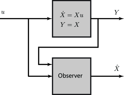
Figure 1: Block diagram of the full state observer setup.

We emphasize that the results of this paper can be extended to right-invariant systems on Lie groups, i.e., systems of the form

$$\dot{X} =uX.$$

However, we restrict the discussion to left-invariant systems to avoid repetition and for clarity.

4.2 Partial state observers

If $\mathsf{G}$ is any linear Lie group then, as we have already seen, its Lie algebra $\operatorname{Lie}(\mathsf{G})$, is a vector space and a subalgebra of $\mathsf{M}\left(n,\mathbb{R}\right)$. Therefore the tangent space at any point $X\in G$ is isomorphic to the Lie algebra itself. This implies that if $c:\mathbb{R}\rightarrow\operatorname{Lie}(\mathsf{G})$ is any smooth curve, then its derivative, $\dot{x}$, is also a curve in $\operatorname{Lie}(\mathsf{G})$, i.e., $\dot{c}:\mathbb{R}\rightarrow\operatorname{Lie}(\mathsf{G})$. Consider the following system

$$\dot{X} =Xx_{2}$$ (9)

$$\dot{x}_{2} =x_{3}$$

$$\;\;\vdots$$

$$\dot{x}_{d} =u$$

$$Y =X,$$

where $X\in\mathsf{G}$ evolves on a linear Lie group and $x_{i}\in\operatorname{Lie}(\mathsf{G})$, $i\in\left\{2,\ldots,d\right\}$. The input to (9) is $u:\mathbb{R}\rightarrow\operatorname{Lie}(\mathsf{G})$ which we assume to be a smooth, uniformly bounded and locally Lipschitz signal of time.

The following assumption, which is almost identical to Assumption 1 in Section 4.1, is assumed throughout this paper.

Assumption 2.

The input $u$ to system (9) is such that for any initial condition $X(0)\in\mathsf{G}$, $x_{2}(0),\ldots,x_{d}(0)\in\operatorname{Lie}(\mathsf{G})$, the corresponding solution $(X(t),x_{2}(t),\ldots,x_{d}(t))$ of (9) is such that $X(t)$ is bounded.

Problem 2: Given the system (8), design a state estimator with estimate $\hat{X}\in\mathsf{G}$, $\hat{x}_{i}\in\operatorname{Lie}{(\mathsf{G})}$, $i\in\left\{2,\ldots,d\right\}$, access to the output $Y\in\mathsf{G}$ and the input $u\in\operatorname{Lie}(\mathsf{G})$, such that, under Assumption 2, if $\|\hat{X}(0)-X(0)\|$, $\|\hat{x}_{2}(0)-x_{2}(0)\|$, $\ldots$, $\|\hat{x}_{d}(0)-x_{d}(0)\|$ are sufficiently small, then $\|\hat{X}(t)-X(t)\|\rightarrow 0$, $\|\hat{x}_{2}(t)-x_{2}(t)\|\rightarrow 0$, $\ldots$, $\|\hat{x}_{d}(t)-x_{d}(t)\|\rightarrow 0$ exponentially, as $t\rightarrow\infty$.

5 Proposed observers

In this section we propose various observers that solve Problems 4.1 and 4.2. The analysis of the observers is presented in Section 8 where, using the results of Section 7, we provide conditions under which the observers solve Problems 4.1 and 4.2.

5.1 Local full state observers

For the system (8), we propose two different observers, which we call local Lie group Full State Observers (LFSOs). The first is the passive LFSO, given by

$$\dot{\hat{X}} =\hat{X}u-a_{0}\hat{X}\log(Y^{-1}\hat{X}).$$ (10)

The second is the direct LFSO, given by

$$\dot{\hat{X}} =YuY^{-1}\hat{X}-a_{0}\hat{X}\log(Y^{-1}\hat{X}).$$ (11)

In the above two observers, the constant $a_{0}>0$ is a design parameter that, as we will show, can be used to change the rate of observer convergence. Following the terminology of [16], we call the term $\alpha(\hat{X},Y)\coloneqq-a_{0}\hat{X}\log(Y^{-1}\hat{X})$, appearing in (10) and (11), the innovation term of the observer. It can be verified that the term $\alpha$ satisfies the definition, given in [16, Definition 15], of an innovation term.

An intuitive and informal explanation for taking this particular form of $\alpha(\hat{X},Y)=-a_{0}\hat{X}\log(Y^{-1}\hat{X})$ is that the matrix $Y^{-1}\hat{X}$ represents a “measurement error” on the Lie group $\mathsf{G}$. The Lie group $\mathsf{G}$ is not a vector space and therefore $Y^{-1}\hat{X}$ is not a vector and should not be added or subtracted with other matrices. To make the matrix $Y^{-1}\hat{X}$ more vector-like, we take its logarithm, which maps it to the vector space $\operatorname{Lie}(\mathsf{G})$, while preserving all its information (since $\log:G\rightarrow\operatorname{Lie}(\mathsf{G})$ is a local diffeomorphism). We then push-forward this vector, $\log(Y^{-1}\hat{X})$, from $T_{I_{n}}G$ to $T_{\hat{X}}G$, the tangent space at $\hat{X}$, by applying the push-forward map of left translation. By Proposition 3.16, left translation from $T_{I_{n}}G$ to $T_{\hat{X}}G$ is the same as left multiplication by $\hat{X}$. The result is a vector in $T_{\hat{X}}G$, which represents the estimation error. This vector-like estimation error is then multiplied by the gain $a_{0}>0$ to adjust the rate of observer convergence.

We call the term $\hat{X}u$ appearing in (10) and the term $YuY^{-1}\hat{X}$ appearing in (11), the synchronization terms of the observer. The choice of synchronization term distinguishes the passive observer from the direct observer.

It is computationally costly and inefficient to compute the matrix logarithm map using the series definitions. Various studies have looked at the problem of approximating this computation. In particular the work [31], [32], [33], [34] may be useful for implementing the observers proposed in this paper. While we do not pursue the notion of using approximations to the matrix logarithm to implement the observers, we do observe, in Section 9, that in the special case $\mathsf{G}=\mathsf{SO}\left(3,\mathbb{R}\right)$ the logarithm can be computed efficiently.

5.2 Local partial state observers

For system (9), we propose two different observers which we call local Lie group Partial State Observers (LPSOs). The first is the direct LPSO, given by

$$\dot{\hat{X}} =Y\hat{x}_{2}Y^{-1}\hat{X}-a_{d-1}\hat{X}\log(Y^{-1}\hat{X})$$ (12)

$$\dot{\hat{x}}_{2} =\hat{x}_{3}-a_{d-2}\log(Y^{-1}\hat{X})$$

$$\vdots$$

$$\dot{\hat{x}}_{d-1} =\hat{x}_{d}-a_{1}\log(Y^{-1}\hat{X})$$

$$\dot{\hat{x}}_{d} =u-a_{0}\log(Y^{-1}\hat{X})$$

and the second is the passive LPSO, given by

$$\dot{\hat{X}} =\hat{X}\hat{x}_{2}-a_{d-1}\hat{X}\log(Y^{-1}\hat{X})$$ (13)

$$\dot{\hat{x}}_{2} =\hat{x}_{3}-a_{d-2}\log(Y^{-1}\hat{X})$$

$$\vdots$$

$$\dot{\hat{x}}_{d-1} =\hat{x}_{d}-a_{1}\log(Y^{-1}\hat{X})$$

$$\dot{\hat{x}}_{d} =u-a_{0}\log(Y^{-1}\hat{X}).$$

In the above two observers, the constants $a_{0},\ldots,a_{d-1}\in\mathbb{R}$ are design parameters, chosen such that the polynomial $p(s)=s^{d}+a_{d-1}s^{d-1}+\cdots+a_{1}s+a_{0}$ is Hurwitz. These design parameters can be used to modify the rate of convergence of the estimation error.

We will show that the direct LPSO (12) is locally exponentially stable for the system (9). Unfortunately we are not able to show exponential stability of the passive LPSO (13). However, we will see in simulation that the passive LPSO works well in the presence of measurement noise.

6 Estimation Error Functions

Following [16], we introduce two canonical choices of estimation error functions for left-invariant systems on Lie groups.

Definition 6.1.

Given system (8) with $X\in\mathsf{G}$, and an observer with state estimate $\hat{X}\in\mathsf{G}$, the canonical left-invariant error, $E_{l}:\mathsf{G}\times\mathsf{G}\rightarrow\mathsf{G}$, is

$$E_{l}(X,\hat{X})\coloneqq X^{-1}\hat{X}$$

and the canonical right-invariant error, $E_{r}:\mathsf{G}\times\mathsf{G}\rightarrow\mathsf{G}$, is

$$E_{r}(X,\hat{X})\coloneqq\hat{X}X^{-1}.$$

The error $E_{l}$ is called left-invariant because, for any $A\in\mathsf{G}$, $E_{l}(AX,A\hat{X})=X^{-1}A^{-1}A\hat{X}=X^{-1}\hat{X}=E_{l}(X,\hat{X})$. Similarly, $E_{r}$ is called right-invariant since, for any $A\in\mathsf{G}$, $E_{r}(XA,\hat{X}A)=E_{r}(X,\hat{X})$. From the definitions of $E_{l}$ and $E_{r}$, it is apparent that

$$E_{r}=\operatorname{Ad}_{X}(E_{l})=XE_{l}X^{-1}$$ (14)

where, for any fixed $X\in\mathsf{G}$, $\operatorname{Ad}_{X}:\mathsf{G}\rightarrow\mathsf{G}$ is a global diffeomorphism.

In Problems 4.1 and 4.2 we seek to design observers so that $\|\hat{X}-X\|\rightarrow 0$ exponentially. To characterize this property we rely on the following result.

Proposition 6.2.

Suppose that $X:\mathbb{R}\to\mathsf{G}$ is bounded. If either $E_{r}\rightarrow I_{n}$ exponentially, or $E_{l}\rightarrow I_{n}$ exponentially, as $t\rightarrow\infty$, then $\hat{X}\rightarrow X$ exponentially, as $t\rightarrow\infty$.

Proof.

For any $X$, $\hat{X}\in\mathsf{G}$, using Definition 6.1, the following identities hold

$$\hat{X}-X =X(X^{-1}\hat{X}-I_{n})=X(E_{l}-I_{n})$$

$$\hat{X}-X =(\hat{X}X^{-1}-I_{n})X=(E_{r}-I_{n})X.$$

Taking the norms of these identities, we obtain

$$\|\hat{X}-X\| \leq\|X\|\|E_{l}-I_{n}\|$$ (15)

$$\|\hat{X}-X\| \leq\|X\|\|E_{r}-I_{n}\|.$$

Additionally, for any $X,\hat{X}\in G$,

$$(E_{l}-I_{n}) =X^{-1}(\hat{X}-X)$$

$$(E_{r}-I_{n}) =(\hat{X}-X)X^{-1}$$

so that

$$\|E_{l}-I_{n}\| \leq\|X^{-1}\|\|\hat{X}-X\|$$ (16)

$$\|E_{r}-I_{n}\| \leq\|X^{-1}\|\|\hat{X}-X\|.$$

By hypothesis, $\|X(t)\|$ is uniformly bounded, i.e., $\left(\exists K_{1}>0\right)$$\left(\forall t\geq 0\right)$$\|X(t)\|\leq K_{1}$. This implies that $X(t)$ evolves on the compact subset $\mathcal{G}=\left\{X\in\mathsf{GL}\left(n,\mathbb{R}\right):\|X\|\leq K_{1}\right\}$. Since the matrix inverse map is continuous, the image of $\mathcal{G}$ under the matrix inverse map is also a compact subset of $\mathsf{GL}\left(n,\mathbb{R}\right)$. Therefore, $\|X^{-1}(t)\|$ is also uniformly bounded, i.e., $\left(\exists K_{2}>0\right)$$\left(\forall t\geq 0\right)$$\|X^{-1}(t)\|\leq K_{2}$.

Now suppose that $\|E_{r}(t)-I_{n}\|\rightarrow 0$ exponentially, as $t\rightarrow\infty$, then by the definition of exponential stability, we have

$$\left(\exists\delta,m,\alpha>0\right)\;\left(\forall E_{r}(0)\in B(I_{n},\delta)\right)\left(\forall t\geq 0\right)\;\|E_{r}(t)-I_{n}\|<me^{-\alpha t}\|E_{r}(0)-I_{n}\|.$$

By the inequalities (15), and uniform boundedness of $\|X\|$, we have that

$$\|E_{r}-I_{n}\|<m\Rightarrow\|\hat{X}-X\|<K_{1}m.$$

By the inequalities (16), and uniform boundedness of $\|X^{-1}\|$, we have that

$$\|\hat{X}-X\|<\frac{\delta}{K_{2}}\Rightarrow\|E_{r}-I_{n}\|<\delta.$$

Combining the above results, we have exponential convergence of $\|\hat{X}-X\|\rightarrow 0$,

$$\left(\exists\delta,m,\alpha>0\right)\left(\|\hat{X}(0)-X(0)\|<\delta/K_{2}\right)$$

$$\qquad\qquad\left(\forall t\geq 0\right)\;\|\hat{X}(t)-X(t)\|<K_{1}K_{2}me^{-\alpha t}\|\hat{X}(0)-X(0)\|.$$

The proof for $E_{l}$ is identical. ∎

In addition to the error functions $E_{l}$ and $E_{r}$, we introduce two other, closely related, error functions.

Definition 6.3.

For any $E_{l}\in B(I_{n},1)$, the log left-invariant error, $e_{l}:\mathsf{G}\times\mathsf{G}\rightarrow\operatorname{Lie}(\mathsf{G})$, is

$$e_{l}(X,\hat{X})\coloneqq\log(E_{l}(X,\hat{X}))=\log(X^{-1}\hat{X}).$$

For any $E_{r}\in B(I_{n},1)$, the log right-invariant error, $e_{r}:\mathsf{G}\times\mathsf{G}\rightarrow\operatorname{Lie}(\mathsf{G})$, is

$$e_{r}(X,\hat{X})\coloneqq\log(E_{r}(X,\hat{X}))=\log(\hat{X}X^{-1}).$$

Since $e_{l}$ is solely a function of $E_{l}$, and since $E_{l}$ is left-invariant, it follows that $e_{l}$ is also left-invariant, i.e. $\forall A\in\mathsf{G}:\;e_{l}(AX,A\hat{X})=e_{l}(X,\hat{X})$. For the same reasoning, it follows that $e_{r}$ is right-invariant, i.e. $\forall A\in\mathsf{G}:\;e_{r}(XA,\hat{X}A)=e_{r}(X,\hat{X})$.

The variables $e_{l}$ and $e_{r}$ are useful because they are vectors in $\operatorname{Lie}(\mathsf{G})$ and they allow us to convert a differential equation on a Lie group into a differential equation on a vector space. The disadvantage of $e_{l}$ and $e_{r}$ is that they are only defined for $E_{l}$, $E_{r}\in B(I_{n},1)$.

Lemma 6.4.

If $E_{l},E_{r}\in B(I_{n},1)$, then

$$e_{r} =Xe_{l}X^{-1}.$$

Proof.

With the help of Lemma 3.12 (d), we obtain

$$e_{r} =\log(E_{r})$$

$$=\log(XE_{l}X^{-1})$$

$$=X\log(E_{l})X^{-1}$$

$$=Xe_{l}X^{-1}.$$

∎

Finally, in the context of partial state observers, since $x_{i}$ and $\hat{x}_{i}$, for $i=2,\ldots,d$ are vectors in $\operatorname{Lie}(\mathsf{G})$, to quantify the error between $x_{i}$ and $\hat{x}_{i}$, we can use subtraction of vectors

$$e_{i}\coloneqq x_{i}-\hat{x}_{i},\hskip 8.53581pti=2,\ldots,d.$$ (17)

Since $x_{i}$ and $\hat{x}_{i}$ are elements of the vector space $\operatorname{Lie}(\mathsf{G})$, $e_{i}$ is also an element of $\operatorname{Lie}(\mathsf{G})$.

7 Differential Equations on Matrices

In this section we study the properties of a pair of differential equations on linear Lie groups. These differential equations arrise in the analysis of the error dynamics associated with the observers proposed in Section 5.

7.1 A Differential Equation on $\mathsf{GL}\left(n,\mathbb{R}\right)$

Consider the differential equation evolving on $\mathsf{GL}\left(n,\mathbb{R}\right)$ given by

$$\dot{E} =-a_{0}E\log(E),$$ (18)

where $E\in\mathsf{GL}\left(n,\mathbb{R}\right)$ and $a_{0}\in\mathbb{R}$ is a positive constant. The equation (18) arises in the analysis of the error dynamics associated with the observers (10), (11). Note that, by Theorem 3.13, the above equation can be written $\dot{E}=-a_{0}\log(E)E$.

While we have defined (18) to evolve on the set of all invertible matrices, $\mathsf{GL}\left(n,\mathbb{R}\right)$. If $\mathsf{G}\subseteq\mathsf{GL}\left(n,\mathbb{R}\right)$ is any linear Lie group, then the vector field (18) is tangent to the submanifold $\mathsf{G}$. Therefore, the submanifold $\mathsf{G}$ is positively invariant for (18). To see that the vector field (18) is tangent to any linear Lie group $\mathsf{G}$, suppose that $E(t_{0})\in\mathsf{G}$ at some time $t_{0}\in\mathbb{R}$. Then $\log(E(t_{0}))\in\operatorname{Lie}(\mathsf{G})$ and left-translation of this vector takes it to the tangent space to $\mathsf{G}$ at $E(t_{0})$, i.e., $E(t_{0})\log(E(t_{0}))\in T_{E(t_{0})}\mathsf{G}$, by Proposition 3.16. Thus, the vector field (18) is such that $\dot{E}(t_{0})\in T_{E(t_{0})}\mathsf{G}$.

The crucial property of the differential equation (18) is that the matrices $\dot{E}$ and $E$ commute, i.e., $E\dot{E}=\dot{E}E$. This property is a consequence of matrices $E$ and $\log(E)$ commuting. Commutativity of $\dot{E}$ and $E$, combined with the product rule, gives us the following result.

Lemma 7.1.

Let $E:\mathbb{R}\rightarrow\mathsf{GL}\left(n,\mathbb{R}\right)$ be a curve in $\mathsf{GL}\left(n,\mathbb{R}\right)$, such that $E$ and $\dot{E}$ commutes. Then for all positive integers $k$

$$\frac{\mathrm{d}}{\mathrm{d}t}\left[(E-I_{n})^{k}\right]=k\dot{E}(E-I_{n})^{k-1}=k(E-I_{n})^{k-1}\dot{E}.$$

Proof.

By straight-forward computation, using the product rule and commutativity of $\dot{E}$ and $E$, we get

$$\frac{\mathrm{d}}{\mathrm{d}t}\left[(E-I_{n})^{k}\right] =\frac{\mathrm{d}}{\mathrm{d}t}\left[\overbrace{(E-I_{n})(E-I_{n})\cdots(E-I_{n})}^{\text{k times }}\right]$$

$$=\overbrace{\dot{E}(E-I_{n})^{k-1}+(E-I_{n})\dot{E}(E-I_{n})^{k-2}+\cdots+(E-I_{n})^{k-1}\dot{E}}^{\text{k times}}$$

$$=k\dot{E}(E-I_{n})^{k-1}$$

$$=k(E-I_{n})^{k-1}\dot{E}.$$

∎

Lemma 7.1 is the key reason why (18) is differentially equivalent to a linear differential equation. The change of coordinates that realizes this equivalence is the matrix logarithm map defined on $B(I_{n},1)\subset\mathsf{GL}\left(n,\mathbb{R}\right)$. By Lemma 3.12, the matrix logarithm map $\log:B(I_{n},1)\rightarrow\mathsf{M}\left(n,\mathbb{R}\right)$ is a diffeomorphism onto its image. Furthermore, the codomain of the $\log$ map is the set $\mathsf{M}\left(n,\mathbb{R}\right)$, which is isomorphic to $\mathbb{R}^{n^{2}}$, as a vector space. Therefore, the $\log$ map is a local coordinate transformation on $\mathsf{GL}\left(n,\mathbb{R}\right)$, defined on the ball $B(I_{n},1)$.

We denote by $e\in\mathsf{M}\left(n,\mathbb{R}\right)$ the $\log$ coordinates of the matrix $E\in B(I_{n},1)$

$$e\coloneqq\log(E).$$ (19)

To express the differential equation (18) in $\log$ coordinates we differentiate $e$ with respect to time, making use of Lemma 7.1 and Proposition 3.1

$$\dot{e} =\frac{\mathrm{d}}{\mathrm{d}t}\log(E)$$

$$=\frac{\mathrm{d}}{\mathrm{d}t}\left[\sum_{k=1}^{\infty}\frac{(-1)^{k+1}}{k}(E-I_{n})^{k}\right]$$

$$=\sum_{k=1}^{\infty}\frac{(-1)^{k+1}}{k}\frac{\mathrm{d}}{\mathrm{d}t}\left[(E-I_{n})^{k}\right]$$

$$=\sum_{k=1}^{\infty}\frac{(-1)^{k+1}}{k}\left[k\dot{E}(E-I_{n})^{k-1}\right]$$

$$=\sum_{k=0}^{\infty}(-1)^{k}(E-I_{n})^{k}\dot{E}$$

$$=E^{-1}\dot{E}$$

$$=-a_{0}E^{-1}E\log(E)$$

$$=-a_{0}e.$$

The above equation, rewritten $\dot{e}=-a_{0}e$, is linear with $n^{2}$ eigenvalues located at $-a_{0}$. Thus, for any positive constant $a_{0}>0$, the point $e=0_{n}$ is an exponentially stable equilibrium of $\dot{e}=-a_{0}e$. Since stability of an equilibrium is a coordinate independent property, the equilibrium point $E=I_{n}$ is also locally exponentially stable for (18). The above discussion proves the following.

Lemma 7.2.

On the set $E\in B(I_{n},1)$, the vector field (18) is differentially equivalent to the vector field

$$\dot{e} =-a_{0}e,$$ (20)

where $e\coloneqq\log(E)$. If $a_{0}>0$, the equilibrium point $E=I_{n}$ of (18) is locally exponentially stable.

The solution, $E(t)$, of the differential equation (18) can be expressed in closed form. This is useful in obtaining an intuitive understanding of the equation (18), but is not necessary for our main argument.

Proposition 7.3.

Let $E_{0}\in B(I_{n},1)$ be sufficiently close to $I_{n}$ so that $\log(E_{0})\in B(0_{n},\log(2))$ and let $a_{0}>0$ be arbitrary. Then the solution of (18) with initial condition $E(0)=E_{0}$ is defined for all $t\geq 0$ and is given by

$$E(t) =\exp(\exp(-a_{0}t)\log(E_{0})).$$ (21)

Proof.

First, we will show that the candidate solution (21) is a solution to the differential equation (18) with initial condition $E_{0}$. First, we check the initial condition. The value at $t=0$ of $E(t)$ is $E(0)=E_{0}$ as required.

Next, we check that $E(t)$ satisfies (18). Differentiate $E(t)$ with respect to time

$$\frac{\mathrm{d}}{\mathrm{d}t}E(t) =\frac{\mathrm{d}}{\mathrm{d}t}\left[\exp(\exp(-a_{0}t)\log(E_{0}))\right]$$

$$=-a_{0}\exp(-a_{0}t)\log(E_{0})\exp(\exp(-a_{0}t)\log(E_{0}))$$

$$=-a_{0}\log(E)E,$$

where we have used the identity

$$\log(E)=\log(\exp(\exp(-a_{0}t)\log(E_{0})))=\exp(-a_{0}t)\log(E_{0}),$$

which follows from Lemma 3.12 (b) and the assumption that $\log(E_{0})\in B(0_{n},\log(2))$.

To finish the proof, let us check that the solution $E(t)$ of (18), with initial condition $E_{0}$ as stated in the proposition, is such that for all future times $t>0$, we have $E(t)\in B(I_{n},1)$. The solution of the linear differential equation (20) is $e(t)=e(0)\exp(-a_{0}t)$, where $e(0)=\log(E_{0})$. Using the fact that $E(t)=\exp(e(t))$, we compute upper bound on $\|E(t)-I_{n}\|$, for $t\geq 0$:

$$\|E(t)-I_{n}\| =\left\|\sum_{k=0}^{\infty}\frac{1}{k!}e(0)^{k}\exp(-a_{0}tk)-I_{n}\right\|$$

$$=\left\|\sum_{k=1}^{\infty}\frac{1}{k!}e(0)^{k}\exp(-a_{0}tk)\right\|$$

$$\leq\sum_{k=1}^{\infty}\frac{1}{k!}\left\|e(0)\right\|^{k}\exp(-a_{0}tk)$$

$$\leq\sum_{k=1}^{\infty}\frac{1}{k!}\left\|e(0)\right\|^{k}$$

$$=\exp(\left\|e(0)\right\|)-1$$

$$<2-1=1.$$

The last inequality follows from the assumption that $\log(E_{0})\in B(0_{n},\log(2))$. Thus, $E(t)\in B(I_{n},1)$ for all $t\geq 0$. ∎

Let $E(t)$ be a solution of (18), which is initialized at $E_{0}=E(0)$, such that the conditions of Proposition 7.3 are satisfied. Then, for all $t\geq 0$, $E(t)$ stays on the same one-parameter subgroup, on which it was initialized at time $t=0$. Indeed, by Proposition 7.3, we have

$$\left(\forall t\geq 0\right)\;\left(\exists\tau\in\mathbb{R}\right)\;\hskip 8.53581ptE(t)=\exp(\tau\log(E_{0})).$$

Thus, in a neighbourhood of $I_{n}\in\mathsf{GL}\left(n,\mathbb{R}\right)$, the vector field (18) is a linear vector field on Lie group, since its flow is a one-parameter subgroup [17], [18].

7.2 A Differential Equation on $\mathsf{GL}\left(n,\mathbb{R}\right)$ and $\mathsf{M}\left(n,\mathbb{R}\right)$

Consider the following differential equation, which is a natural extension of the differential equation (18),

$$\dot{E} =e_{2}E-a_{d-1}E\log(E)$$ (22)

$$\dot{e}_{2} =e_{3}-a_{d-2}\log(E)$$

$$\vdots$$

$$\dot{e}_{d-1} =e_{d}-a_{1}\log(E)$$

$$\dot{e}_{d} =-a_{0}\log(E),$$

where $E\in\mathsf{GL}\left(n,\mathbb{R}\right)$, $e_{i}\in\mathsf{M}\left(n,\mathbb{R}\right)$ for $i=2,\ldots,d$ and $a_{0},\ldots,a_{d-1}\in\mathbb{R}$ are constants such that the polynomial $p(s)=s^{d}+a_{d-1}s^{d-1}+\cdots+a_{1}s+a_{0}$ is Hurwitz. System (22) arises in the analysis of the error dynamics associated with the direct LPSO (12).

Remark 7.4.

Let $\mathsf{G}\subseteq\mathsf{GL}\left(n,\mathbb{R}\right)$ be any linear Lie group, then the embedded submanifold, $S\coloneqq\mathsf{G}\times\operatorname{Lie}(\mathsf{G})\times\cdots\times\operatorname{Lie}(\mathsf{G})$, in the state space of (22) is positively invariant under the dynamics (22). To see this, we check that, if $p=(E,e_{2},\ldots,e_{d})\in S$, then the vector field (22), evaluated at $p$, lies in the tangent space to $S$ at $p$.

Indeed, by Proposition 3.16, we have that $E\log(E)\in T_{E}G$ and that $e_{2}E\in T_{E}G$. Therefore, the vector $\dot{E}=e_{2}E-a_{d-1}E\log(E)$ is in the tangent space to $\mathsf{G}$ at $E$, i.e., $\dot{E}\in T_{E}\mathsf{G}$. Furthermore we have that, for $i=2,\ldots,d$, $\dot{e}_{i}\in\operatorname{Lie}(\mathsf{G})\simeq T_{e_{i}}\operatorname{Lie}(\mathsf{G})$, because $\operatorname{Lie}(\mathsf{G})$ is a vector space. So the following holds

$$E\in G,\hskip 8.53581pte_{2}\in \operatorname{Lie}(G),\hskip 8.53581pt\ldots,\hskip 8.53581pte_{d}\in\operatorname{Lie}(G)$$

$$\Downarrow$$

$$\dot{E}\in T_{E}G,\hskip 8.53581pt\dot{e}_{2}\in T_{e_{2}}\operatorname{Lie}(G),\hskip 8.53581pt\ldots,\hskip 8.53581pt\dot{e}_{d}\in T_{e_{d}}\operatorname{Lie}(G),$$

Therefore, the vector field (22) is tangent to the submanifold $S$.

In general the matrices $E$ and $\dot{E}$ in (22) do not commute. This is because $E$ and $e_{2}$ are generally non-commuting matrices, i.e.,

$$\left[E,\dot{E}\right] =\left[E,e_{2}E-a_{1}E\log(E)\right]$$

$$=\left[E,e_{2}E\right]$$

$$=Ee_{2}E-e_{2}E^{2}$$

$$=\left[E,e_{2}\right]E.$$

The non-commutativity of $E$ and $\dot{E}$ means that, defining $e_{1}\coloneqq\log(E)$, the expression for $\dot{e}_{1}$ is not as simple as was the case for equation (18) in Section 7.1. In particular, we do not obtain a closed-form expression for $\dot{e}_{1}$. Instead we have the following, weaker, result.

Proposition 7.5.

In the open neighbourhood $B(I_{n},1)\times\left(\mathsf{M}\left(n,\mathbb{R}\right)\right)^{d-1}$ the differential equation (22) is differentially equivalent to

$$\dot{e}_{1} =e_{2}-a_{d-1}e_{1}+K(e_{1},e_{2})$$

$$\dot{e}_{2} =e_{3}-a_{d-2}e_{1}$$

$$\vdots$$

$$\dot{e}_{d-1} =e_{d}-a_{1}e_{1}$$

$$\dot{e}_{d} =-a_{0}e_{1},$$

where $e_{1}\coloneqq\log(E)$ and $K:\operatorname{Lie}(G)\times\operatorname{Lie}(G)\rightarrow\operatorname{Lie}(G)$ is a smooth function that vanishes if $e_{1}$ and $e_{2}$ commute, i.e.,

$$\left(\forall\;e_{1},e_{2}\in\mathsf{M}\left(n,\mathbb{R}\right)\;[e_{1},e_{2}]=0_{n}\right)\;K(e_{1},e_{2})=0_{n}.$$

Proof.

Since $e_{1}=\log(E)$ is a Taylor series in $E$, term by term differentiation yields that $\dot{e}_{1}$ only depends on $E$ and $\dot{E}$. Furthermore, from (22), we know that $\dot{E}$ only depends on $E$ and $e_{2}$. Thus, using $E=\exp(e_{1})$, we have that $\dot{e}_{1}$ only depends on $e_{1}$ and $e_{2}$. Let $K(e_{1},e_{2})\coloneqq\dot{e}_{1}-e_{2}+a_{d-1}e_{1}$.

Assume that $e_{1}$ and $e_{2}$ commute. This implies that $E=\exp(e_{1})$ and $e_{2}$ also commute and this implies that $E$ and $\dot{E}$ commute. Since $E\dot{E}=\dot{E}E$, we can repeat almost the same analysis that we used in Section 7.1, doing this we get

$$\dot{e}_{1} =\dot{E}E^{-1}$$

$$=e_{2}-a_{d-1}e_{1},$$

therefore $K(e_{1},e_{2})=0_{n}$ for any commuting $e_{1}$ and $e_{2}$.

The expressions of $\dot{e}_{i}$ for $i=2,\ldots,d$ are computed by substituting $\log(E)=e_{1}$ into (22). ∎

Lemma 7.6.

If the constants $a_{0},\ldots,a_{d-1}\in\mathbb{R}$ are chosen such that the polynomial $p(s)=s^{d}+a_{d-1}s^{d-1}+\cdots+a_{1}s+a_{0}$ is Hurwitz then the equilibrium point $(E,e_{2},\ldots,e_{d})=(I_{n},0_{n},\ldots,0_{n})$ of the differential equation (22) is locally exponentially stable.

Proof.

Adapting the proof of [15, Theorem 3.1 (ii)], we show that (22) is locally exponentially stable at the equilibrium point, by showing that its linearization, around the equilibrium point $(I_{n},0_{n},\ldots,0_{n})$, is exponentially stable.

In a neighbourhood of the equilibrium point $(I_{n},0_{n},\ldots,0_{n})$ define

$$\delta E\coloneqq E-I_{n},\hskip 19.91692pt\delta e_{2}\coloneqq e_{2}-0_{n},\hskip 19.91692pt\ldots,\hskip 19.91692pt\delta e_{d}\coloneqq e_{d}-0_{n}.$$

Using the series definition of the matrix logarithm (7)

$$\log(E)=\delta E-\frac{1}{2}(\delta E)^{2}+\cdots$$

we deduce that, near $\delta E=0_{n}$,

$$\log(E)\approx\delta E.$$

Similarly, using $E=\delta E+I_{n}$, and dropping higher order terms in $\delta E$, we get

$$E\log(E)=(\delta E+I_{n})\left((\delta E)-\frac{1}{2}(\delta E)^{2}+\cdots\right)\approx\delta E.$$

Finally, near the equilibrium point $(I_{n},0_{n},\ldots,0_{n})$,

$$e_{2}E=\left(\delta e_{2}\right)\left(\delta E+I_{n}\right)\approx\delta e_{2}.$$

Substituting these approximations into the differential equation (22), we get the linearization of (22) at $(I_{n},0_{n},\ldots,0_{n})$

$$\frac{\mathrm{d}}{\mathrm{d}t}\left[\begin{array}[]{c}\delta E\\ \delta e_{2}\\ \delta e_{3}\\ \vdots\\ \delta e_{d-1}\\ \delta e_{d}\end{array}\right]=\left(\begin{array}[]{cccccc}-a_{d-1}I_{n}&I_{n}&0_{n}&\ldots&0_{n}&0_{n}\\ -a_{d-2}I_{n}&0_{n}&I_{n}&\ldots&0_{n}&0_{n}\\ -a_{d-3}I_{n}&0_{n}&0_{n}&\ldots&0_{n}&0_{n}\\ \vdots&\vdots&\vdots&\ddots&\vdots&\vdots\\ -a_{1}I_{n}&0_{n}&0_{n}&\ldots&0_{n}&I_{n}\\ -a_{0}I_{n}&0_{n}&0_{n}&\ldots&0_{n}&0_{n}\end{array}\right)\left[\begin{array}[]{c}\delta E\\ \delta e_{2}\\ \delta e_{3}\\ \vdots\\ \delta e_{d-1}\\ \delta e_{d}\end{array}\right].$$

The eigenvalues of the system matrix are located at the roots of the polynomial $p(s)=s^{d}+a_{d-1}s^{d-1}+\cdots+a_{1}s+a_{0}$, with multiplicity $n$, for each (possibly repeating) root of $p(s)$. Since all the eigenvalues have negative real parts, the linearization above is exponentially stable. Therefore $(E,e_{2},\ldots,e_{d})=(I_{n},0_{n},\ldots,0_{n})$ is a locally exponentially stable equilibrium of (22). ∎

8 Estimation Error Dynamics

In this section we analyse the stability of the estimation error for the each of the observers proposed in Section 5. We show that, under Assumptions 1 and 2, the estimates exponentially converge to the state of the system.

8.1 Local full state observers

We first analyze the dynamics of the error functions $E_{l}$ and $E_{r}$ under the observers defined by (10) and (11). Our analysis makes frequent use of Lemma 3.7. We assume that $\hat{X}$ is initialized sufficiently close to $X$, so that $E_{l}$, $E_{r}\in B(I_{n},1)$. This assumption is sufficient to ensure that the series definitions, using (7), of $\log(E_{r})$ and $\log(E_{l})$ are convergent.

8.1.1 Passive Observer

When the passive observer (10) is used to estimate the state of (8) dynamics of the right-invariant error, $E_{r}$, making use of Lemma 3.7, are

$$\dot{E}_{r} =\frac{d}{dt}\left[\hat{X}X^{-1}\right]$$ (23)

$$=\dot{\hat{X}}X^{-1}-\hat{X}X^{-1}\dot{X}X^{-1}$$

$$=\hat{X}uX^{-1}-a_{0}\hat{X}\log(X^{-1}\hat{X})X^{-1}-\hat{X}uX^{-1}$$

$$=-a_{0}\hat{X}\log(X^{-1}\hat{X})X^{-1}$$

$$=-a_{0}\hat{X}X^{-1}X\log(X^{-1}\hat{X})X^{-1}$$

$$=-a_{0}\hat{X}X^{-1}\log(\hat{X}X^{-1})$$

$$=-a_{0}E_{r}\log(E_{r}).$$

The above differential equation is formally the same as equation (18). Therefore if $\hat{X}$ is sufficiently close to $X$ so that $E_{r}\in B(I_{n},1)$ then, by Lemma 7.2, system (23) is differentially equivalent to

$$\dot{e}_{r}=-a_{0}e_{r},.$$ (24)

By choosing $a_{0}>0$, Lemma 7.2 states the equilibrium point $E_{r}=I_{n}$ is locally exponentially stable for system (23). This discussion, in light of Proposition 6.2, proves the following solution to Problem (4.1).

Corollary 8.1.

For $E_{r}(0)\in B(I_{n},1)$, the passive observer (10) exponentially stabilizes $E_{r}=I_{n}$. Furthermore, under Assumption 1, the passive observer solves Problem (4.1).

The convergence of $E_{r}$ to $I_{n}$ does not rely on the trajectories of (8) being bounded. Next, we examine the dynamics of the left-invariant error, $E_{l}$, to see if Assumption 1 can be weakened. The dynamics of the left invariant error $E_{l}$ under the passive observer (10) are

$$\dot{E}_{l} =\frac{d}{dt}\left[X^{-1}\hat{X}\right]$$ (25)

$$=-X^{-1}\dot{X}X^{-1}\hat{X}+X^{-1}\dot{\hat{X}}$$

$$=-uX^{-1}\hat{X}+X^{-1}\hat{X}u-a_{0}X^{-1}\hat{X}\log(X^{-1}\hat{X})$$

$$=-uE_{l}+E_{l}u-a_{0}E_{l}\log(E_{l})$$

$$=-a_{0}E_{l}\log(E_{l})+\delta_{P}(u,E_{l}),$$

where $\delta_{P}(u,E_{l})\coloneqq E_{l}u-uE_{l}$ is a perturbation term that vanishes when $E_{l}=I_{n}$. Since the matrices $E_{l}$ and $\dot{E}_{l}$ do not, in general, commute, Lemma 7.1 does not hold for (25).

Next we transform the error dynamics (25) into $\log$ coordinates. Recall, by Lemma 6.4, if $\hat{X}$ is sufficiently close to $X$ then $e_{l}=X^{-1}e_{r}X$. Therefore to transform the dynamics (25) into $e_{l}$ coordinates, we just differentiate this alternate expression for $e_{l}$

$$\dot{e}_{l} =\frac{d}{dt}\left[X^{-1}e_{r}X\right]$$ (26)

$$=-X^{-1}\dot{X}X^{-1}e_{r}X+X^{-1}\dot{e}_{r}X+X^{-1}e_{r}\dot{X}$$

$$=-ue_{l}-a_{0}e_{l}+e_{l}u$$

$$=-a_{0}e_{l}+\left[e_{l},u\right].$$

The above system, rewritten $\dot{e}_{l}=-a_{0}e_{l}+\left[e_{l},u\right]$, is bilinear. If $a_{0}<0$, then by [35, Corollary 4], system (26) is integral-input to state stable (iISS). Specifically, see [35], there exist class-$\mathcal{K}_{\infty}$ functions $\alpha$, $\gamma$ and a class-$\mathcal{KL}$ function $\beta$ such that for any $e_{l}(0)\in\mathsf{M}\left(n,\mathbb{R}\right)$, and any input $u(\cdot)$

$$\alpha(\|e_{l}(t)\|)\leq\beta(e_{l}(0),t)+\int_{0}^{t}\gamma(\|u(\tau)\|)\mathrm{d}\tau.$$

As a result, if $u(t)\to 0_{n}$ as $t\to\infty$, then $e_{l}(t)\to 0_{n}$ as $t\to\infty$. Furthermore, if $\int^{\infty}_{0}\gamma(\|u(t)\|)\mathrm{d}t<\infty$, then by [35, Proposition 6], $e_{l}(t)\to 0_{n}$ as $t\to\infty$. Niether of these properties allow us to weaken Assumption 1. First, because we have no guarantees that the control signal satisfies the above properties and second, System (25) is only differentially equivalent to (26) if $E_{l}\in B(I_{n},1)$ and the iISS property does not ensure that $e_{l}\in\log{(B(I_{n},1))}$.

By showing that the system (25) is diffeomorphic to the system (26), we have found an easy way to prove the following, non-obvious, result.

Corollary 8.2.

Let $G\subseteq\mathsf{GL}\left(n,\mathbb{R}\right)$ be a linear Lie group and consider the system

$$\dot{E}=[E,u],$$ (27)

where $E\in\mathsf{G}\subseteq\mathsf{GL}\left(n,\mathbb{R}\right)$ is the state and $u\in\operatorname{Lie}(G)\subseteq\mathsf{M}\left(n,\mathbb{R}\right)$ is an admissible input signal. On the open set $B(I_{n},1)\cap\mathsf{G}$, system (27) is differentially equivalent to

$$\dot{e}=[e,u],$$ (28)

where $e=\log(E)$.

Proof.

Rewrite (27) as a difference of two vector fields

$$\dot{E} =\left([E,u]+E\log(E)\right)-\left(E\log(E)\right)$$

$$=f(E,u)-g(E),$$

where $f(E,u)\coloneqq[E,u]+E\log(E)$ and $g(E)\coloneqq E\log(E)$. Since the system (25) transforms into the system (26), we know that the vector field $f(E,u)$ transforms into $[e,u]+e$. Also, since the dynamics (18) transform into the dynamics (20), we know that the vector field $g(E)$ transforms into $e$. This means that the vector field $f(E,u)-g(E)$ transforms into $[e,u]+e-e=[e,u]$. ∎

Recall, that in equation (18), we were able to easily differentiate the Taylor series expansion of $\log(E)$, because the matrices $E$ and $\dot{E}=-a_{0}E\log(E)$ commute, i.e., $E\dot{E}=\dot{E}E$. However, in the equation (27), the matrices $E$ and $\dot{E}=[E,u]$ do not commute, i.e., in general $E\dot{E}\neq\dot{E}E$. This non-commutativity makes it very difficult to differentiate the Taylor series expansion of $\log(E)$, when $\dot{E}=[E,u]$, as in (27). Thus, it seems that the result of Corollary 8.2 is difficult to directly obtain by differentiating the series expansion of $\log(E)$ and substituting $\dot{E}=[E,u]$. Our analysis of equation (27) is facilitated by taking the systemic view of “splitting” the equation (27) into a pair consisting of “system” (8), with state $X$, and “observer” (10), with state $\hat{X}$. The splitting is done as $E=X^{-1}\hat{X}$, and allows us to convert the differential equation (27) into $\log$ coordinates.

8.1.2 Direct Observer

When the direct observer (11) is used to estimate the state of (8) dynamics of the left-invariant error, $E_{l}$, making use of Lemma 3.7, are

$$\dot{E}_{l} =\frac{d}{dt}\left[X^{-1}\hat{X}\right]$$ (29)

$$=-X^{-1}\dot{X}X^{-1}\hat{X}+X^{-1}\dot{\hat{X}}$$

$$=-uX^{-1}\hat{X}+uX^{-1}\hat{X}-a_{0}X^{-1}\hat{X}\log(X^{-1}\hat{X})$$

$$=-uE_{l}+uE_{l}-a_{0}E_{l}\log(E_{l})$$

$$=-a_{0}E_{l}\log(E_{l}).$$

The above equation (29) is the same as the equation (18), if we identify $E_{l}$ with $E$. This means that if $\hat{X}$ is sufficiently close to $X$ so that $E_{l}\in B(I_{n},1)$, then by Lemma 7.2, system (29) in $e_{l}$-coordinates reads

$$\dot{e}_{l}=-a_{0}e_{l}.$$ (30)

If $a_{0}>0$, Lemma 7.2 states that the equilibrium point $E_{l}=I_{n}$ is locally exponentially stable for the dynamics (29).

Corollary 8.3.

For $E_{l}(0)\in B(I_{n},1)$, the direct observer (10) exponentially stabilizes $E_{l}=I_{n}$. Furthermore, under Assumption 1, the passive observer solves Problem (4.1).

As before, we seek to weaken Assumption 1 and hence we examine the dynamics of the right-invariant error $E_{r}$, when the direct observer is used

$$\dot{E}_{r} =\frac{d}{dt}\left[\hat{X}X^{-1}\right]$$ (31)

$$=\dot{\hat{X}}X^{-1}-\hat{X}X^{-1}\dot{X}X^{-1}$$

$$=XuX^{-1}\hat{X}X^{-1}-a_{0}\hat{X}\log(X^{-1}\hat{X})X^{-1}-\hat{X}uX^{-1}$$

$$=XuX^{-1}E_{r}-E_{r}XuX^{-1}-a_{0}E_{r}X\log(E_{l})X^{-1}$$

$$=XuX^{-1}E_{r}-E_{r}XuX^{-1}-a_{0}E_{r}\log(E_{r})$$

$$=\delta_{D}(u,X,E_{r})-a_{0}E_{r}\log(E_{r}).$$

Here, $\delta_{D}(u,X,E_{r})\coloneqq XuX^{-1}E_{r}-E_{r}XuX^{-1}$ is a perturbation term that vanishes when $E_{r}=I_{n}$. The above equation (31) has the same problem that we encountered when trying to analyze equation (25). Namely, the matrices $E_{r}$ and $\dot{E}_{r}$ do not commute in general, because $E_{r}$ and $\delta_{D}(u,X,E_{r})$ do not commute in general. Fortunately, we can transform equation (25) into $\log$ coordinates by once again differentiating the identity $e_{r}=Xe_{l}X^{-1}$. To be able to do this, it is sufficient that the conditions of Lemma 6.4 are satisfied, i.e., that $E_{l},E_{r}\in B(I_{n},1)$. Doing so, one obtains

$$\dot{e}_{r} =\frac{d}{dt}\left[Xe_{l}X^{-1}\right]$$ (32)

$$=\dot{X}e_{l}X^{-1}+X\dot{e}_{l}X^{-1}-Xe_{l}X^{-1}\dot{X}X^{-1}$$

$$=Xue_{l}X^{-1}-a_{0}Xe_{l}X^{-1}-Xe_{l}uX^{-1}$$

$$=-a_{0}e_{r}+\left[XuX^{-1},e_{r}\right].$$

The above system, rewritten $\dot{e}_{r}=-a_{0}e_{r}+\left[XuX^{-1},e_{r}\right]$, is a non-autonomous, bilinear system. Once again, we cannot weaken the requirement of Assumption 1 and rely on Proposition 6.2 to ensure that $E_{l}\to 0_{n}$ as $t\to\infty$ is equivalent to $E_{r}\to 0_{n}$ as $t\to\infty$.

8.2 Local partial state observers

We now analyze the estimation error dynamics when using the observers proposed in Section 5.2 and defined by (13) and (12).

8.2.1 Direct Observer

When the direct observer (12) is applied to estimate the state of system (9) the dynamics of the right-invariant error $E_{l}$ are

$$\dot{E}_{l} =e_{2}E_{l}-a_{d-1}E_{l}\log(E_{l})$$ (33)

$$\dot{e}_{2} =e_{3}-a_{d-2}\log(E_{l})$$

$$\vdots$$

$$\dot{e}_{d-1} =e_{d}-a_{1}\log(E_{l})$$

$$\dot{e}_{d} =-a_{0}\log(E_{l}).$$

The above differential equation is formally the same as equation (22), if we identify $E$ with $E_{l}$. Application of Lemma 7.6 immediately yields the following solution to Problem 4.2.

Corollary 8.4.

For $(E_{l},e_{2},\ldots,e_{d})\in B(I_{n},I)\times\left(\mathsf{M}\left(n,\mathbb{R}\right)\right)$, the direct observer (12) exponentially stabilizes $(I_{n},0_{n},\ldots,0_{n})$. Furthermore, under Assumption 2, the direct observer solves Problem 4.2.

8.2.2 Passive Observer

When the passive observer (13) is employed to estimate the state of system (9) the dynamics of the right-invariant error $E_{r}$ are given by

$$\dot{E}_{r} =E_{r}\operatorname{Ad}_{X}(e_{2})-a_{d-1}E_{r}\log(E_{r})$$ (34)

$$\dot{e}_{2} =e_{3}-a_{d-2}\log(E_{r})$$

$$\vdots$$

$$\dot{e}_{d-1} =e_{d}-a_{1}\log(E_{r})$$

$$\dot{e}_{d} =-a_{0}\log(E_{r}).$$

Lemma 7.6 cannot be used to deduce the stability of the equilibrium point $(E_{r},e_{2},\ldots,e_{d})=(I_{n},0_{n},\ldots,0_{n})$. Unfortunately, we are not able to prove the stability of these error dynamics. We conjecture that the passive LPSO is locally exponentially convergent if Assumption 2 holds. This conjecture is supported by simulation, where the passive LPSO performs better than the direct LPSO, when a large amount of measurement noise is present in $Y$.

9 Examples

9.1 State estimation on $\mathsf{SO}\left(3,\mathbb{R}\right)$

Recall the kinematic model of a rotating rigid body  (1) introduced in Section 2. For the kinematics (1), the proposed passive observer is

$$\dot{\hat{R}} =\hat{R}\omega+a_{0}\hat{R}\log(Y^{\top}\hat{R}),$$ (35)

and the direct observer is

$$\dot{\hat{R}} =Y\omega Y^{\top}\hat{R}+a_{0}\hat{R}\log(Y^{\top}\hat{R}).$$ (36)

We now briefly discuss the connection between our two observers and the filters from [3], [4]. The authors propose passive and direct filters that are similar to the ones proposed herein. The passive filter of [3], [4] is

$$\dot{\hat{R}} =\hat{R}\omega+k\hat{R}\pi_{a}(\hat{R}^{\top}R),$$ (37)

and the direct filter of [3], [4] is

$$\dot{\hat{R}} =\operatorname{Ad}_{R}(\omega)\hat{R}+k\operatorname{Ad}_{\hat{R}}(\pi_{a}(\hat{R}^{\top}R))\hat{R}$$ (38)

$$=R\omega R^{\top}\hat{R}+k\hat{R}\pi_{a}(\hat{R}^{\top}R),$$

where $k\in\mathbb{R}$ is a positive constant that controls the rate of observer convergence and $\pi_{a}:\mathsf{M}\left(n,\mathbb{R}\right)\to\operatorname{Lie}(\mathsf{SO}\left(3,\mathbb{R}\right))$, $A\mapsto\frac{1}{2}(A-A^{T})$ is the anti-symmetric projection operator.

The synchronization terms of the two passive observers (35) and (37) are the same: $\hat{R}\omega$. The synchronization terms of the two direct observers (36) and (38) are also the same: $R\omega R^{T}\hat{R}$. However, the innovation term of our proposed observer, when applied to $\mathsf{SO}\left(3,\mathbb{R}\right)$ is different from the innovation term of the observers proposed in [3], [4]. In particular, for any $A\in\mathsf{SO}\left(3,\mathbb{R}\right)$ we can express $\log{(A)}$ in terms of the anti-symmetric projection operator using [3, Section III. C.]

$$\pi_{a}(A)=\frac{\sin(\theta_{A})}{\theta_{A}}\log(A)$$ (39)

where $\theta_{A}$ is the rotation angle corresponding to the axis-angle representation of $A$. The angle $\theta_{A}$ can be computed [36] as $\theta_{A}\coloneqq\arccos\left(\frac{\operatorname{trace}(A)-1}{2}\right)$.

Using the identity (39), we can express the observers (35) and (36) in terms of the anti-symmetric projection operator, rather than the logarithm map. For $\theta_{Y^{\top}\hat{R}}\neq\pm\pi$, the passive LFSO (35) is rewritten as

$$\dot{\hat{R}} =\hat{R}u-a_{0}\frac{\theta_{Y^{\top}\hat{R}}}{\sin(\theta_{Y^{\top}\hat{R}})}\hat{R}\pi_{a}(Y^{\top}\hat{R})$$ (40)

and the direct LFSO (36) is rewritten as

$$\dot{\hat{R}} =YuY^{\top}\hat{R}-a_{0}\frac{\theta_{Y^{\top}\hat{R}}}{\sin(\theta_{Y^{\top}\hat{R}})}\hat{R}\pi_{a}(Y^{\top}\hat{R}).$$ (41)

If we take the observer gains to be equal $k=a_{0}$, then (40), (41) differ from (37), (38) by the scalar quantity $\frac{\theta_{Y^{\top}\hat{R}}}{\sin(\theta_{Y^{\top}\hat{R}})}$, which appears in the innovation terms of (40), (41), but does not appear in the innovation terms of (37), (38). This scalar quantity approaches $1$ as $\theta_{Y^{\top}\hat{R}}$ approaches $0$. Thus, on $\mathsf{SO}\left(3,\mathbb{R}\right)$ and for small $\theta_{Y^{\top}\hat{R}}$, our observers behave similar to the observers of [3], [4].

We now simulate our direct and passive LFSOs. The initial conditions for the plant and the observer are chosen as

$$R(0)=\left(\begin{array}[]{ccc}0.6330&-0.1116&-0.7660\\ 0.7128&-0.3020&0.6330\\ -0.3020&-0.9467&-0.1116\end{array}\right),\qquad\hat{R}(0)=I_{3}.$$

The angular velocity input is as

$$u(t)=\left(\begin{array}[]{ccc}0&-2\sin(t)&\cos(t)\\ 2\sin(t)&0&-\sin(t)\\ -\cos(t)&\sin(t)&0\end{array}\right).$$

The observer gain is taken to be $a_{0}=1$. Figure 2 shows the simulation results when there is no noise, i.e., when $Y$ is exactly equal to $R$. From these plots we see that, when there no measurement noise, the direct and passive LFSOs have similar performance.

The Lie group estimation errors, $E_{l}$ and $E_{r}$, are initially (at time $t=0$) $E_{l}(0)=R^{-1}(0)\hat{R}(0)=R^{-1}(0)$, and $E_{r}(0)=\hat{R}(0)R^{-1}(0)=R^{-1}(0)$. Calculating the distance between $E_{l}(0)$ or $E_{r}(0)$ and $I_{3}$, we get $\|E_{l}(0)-I_{3}\|=\|E_{r}(0)-I_{3}\|=1.6675$. Therefore $E_{l}(0),E_{r}(0)\notin B(I_{3},1)$. Strictly speaking, our analysis of the Lie group estimation error dynamics was performed on the ball $B(I_{n},1)$. The simulation shows that that the LFSOs are nevertheless convergent and suggests that the region of convergence of the LFSO is larger than $B(I_{n},1)$.

Figure 3 shows simulations of our observers in the presence of measurement noise. The noisy measurement $Y$ is obtained by multiplying $R$ by a randomly generated rotation matrix $N$, to obtain: $Y=RN$. To generate the random rotation matrix $N\in\mathsf{SO}\left(3,\mathbb{R}\right)$, we generate a random skew-symmetric matrix, $n\in\operatorname{Lie}(\mathsf{SO}\left(3\right))$, whose elements are normally distributed, with zero-mean and standard deviation of $\sigma=0.4$. The random rotation matrix $N\in\mathsf{SO}\left(3\right)$ is then computed as $N\mathrel{\mathop{:}}=\exp(n)$.

From Figure 3, we see that the passive observer appears to be more robust with respect to noise than the direct observer. This observation can be explained by noting that when $Y=RN$, the synchronization term $RN\omega N^{\top}R^{\top}$ of the direct observer is explicitly impacted by the noise. The noise has no explicit effect on the synchronization term of the passive observer.

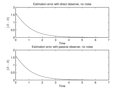
Figure 2: $\|\hat{R}-R\|$ versus time for the proposed LFSO observers on $\mathsf{SO}\left(3,\mathbb{R}\right)$ without measurement noise. Typical result from repeated testing.

Figure 3: $\|\hat{R}-R\|$ versus time for the proposed LFSO observers on $\mathsf{SO}\left(3,\mathbb{R}\right)$ with a significant amount of measurement noise. Typical result from repeated testing.

9.2 Dynamic Rigid-Body Orientation Estimation on $\mathsf{SO}\left(3\right)$

Recall the dynamic model of a rotating rigid body  (2) introduced in Section 2. A similar model was discussed in [37, Example 2]. For system (1), the proposed direct observer is

$$\dot{\hat{R}} =Y\hat{\omega}Y^{-1}\hat{R}-a_{1}\hat{R}\log(Y^{-1}\hat{R})$$ (42)

$$\dot{\hat{\omega}} =u-a_{0}\log(Y^{-1}\hat{R})$$

and the passive LPSO is

$$\dot{\hat{R}} =\hat{R}\hat{\omega}-a_{1}\hat{R}\log(Y^{-1}\hat{R})$$ (43)

$$\dot{\hat{\omega}} =u-a_{0}\log(Y^{-1}\hat{R}).$$

We simulate the direct and the passive LPSOs, with increasing amounts of noise in the output. The initial conditions for the plant and the observer are chosen as

$$R(0)=\left(\begin{array}[]{ccc}0&1&0\\ 0&0&1\\ 1&0&0\end{array}\right),\hskip 8.53581pt\omega(0)=\left(\begin{array}[]{ccc}0&-1&1\\ 1&0&-1\\ -1&1&0\end{array}\right),\hskip 8.53581pt\hat{R}(0)=I_{3},\hskip 8.53581pt\hat{\omega}(0)=0_{3}.$$

The angular acceleration input is chosen to be

$$u(t)=\left(\begin{array}[]{ccc}0&-2\sin(t)&\cos(t)\\ 2\sin(t)&0&-\sin(t)\\ -\cos(t)&\sin(t)&0\end{array}\right).$$

The observer gains are chosen as

$$a_{0}=1,\hskip 19.91692pta_{1}=2.$$

Noise is injected into the output via the random rotation matrix $N\in\mathsf{SO}\left(3,\mathbb{R}\right)$, by setting $Y=RN$. The matrix $N$ is generated as in Section 9.1. The simulation results are shown in Figure 4. From the simulations, when there is no measurement noise, the direct LPSO appears to converge faster than the passive LPSO. However, with a large amount of measurement noise, the passive LPSO appears to be comparable to the direct LPSO.

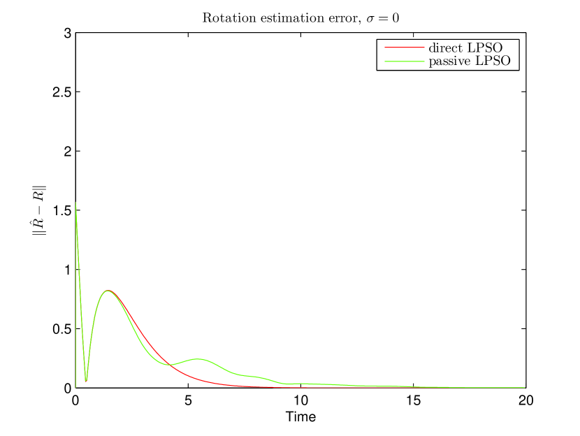
(a) $\|\hat{R}-R\|$ versus time with $\sigma=0$.

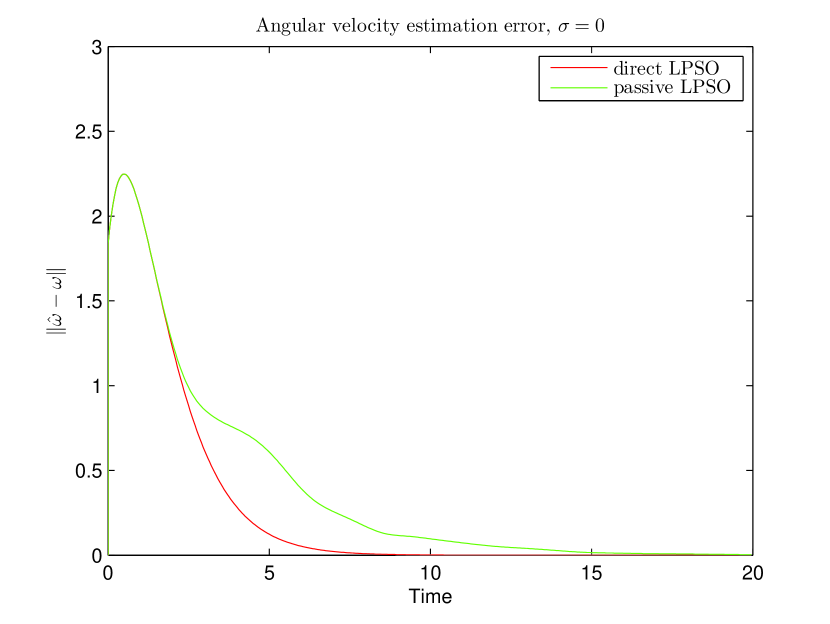
(b) $\|\hat{\omega}-\omega\|$ versus time with $\sigma=0$.

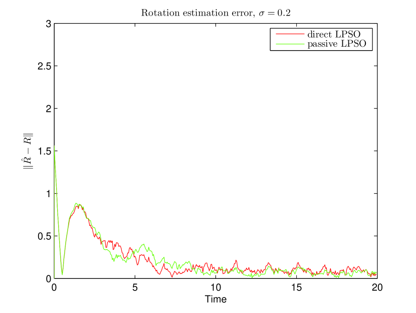
(c) $\|\hat{R}-R\|$ versus time with $\sigma=0.2$.

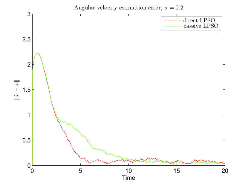
(d) $\|\hat{\omega}-\omega\|$ versus time with $\sigma=0.2$.

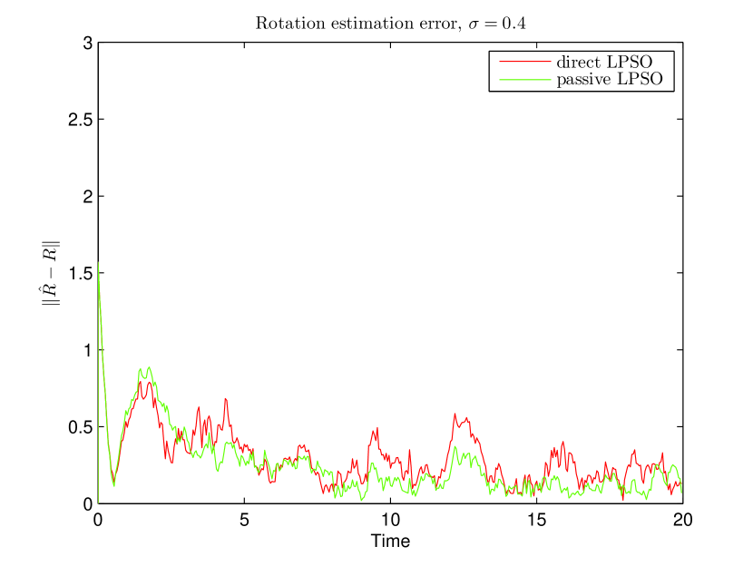
(e) $\|\hat{R}-R\|$ versus time with $\sigma=0.4$.

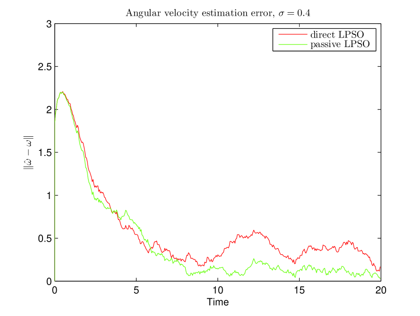
(f) $\|\hat{\omega}-\omega\|$ versus time with $\sigma=0.4$.

Figure 4: Direct and passive LPSOs for dynamic system on $\mathsf{SO}\left(3,\mathbb{R}\right)$ with increasing amounts of measurement noise.

10 Conclusions

We have proposed observers for two different classes of systems on linear Lie groups. The first class of system is one in which the entire state evolves on the general linear group and the entire state is measured. We call observers for this class of system Lie group full-state observers. We have shown that if the systems state is bounded, then both the left and right invariant estimation errors are differentially equivalent to a stable LTI system and hence are locally exponentially stable. The second class of system is one in which only part of the state evolves on the general linear group and only this portion of the state is measured. We call observers for this class of system Lie group partial-state observers. We have shown that if the system’s state is bounded, then the left and right estimation errors are locally exponentially stable using the direct observer. For this class of system the passive observer was shown to work well in simulation. In all cases the observers were shown to work well in simulation in the presence of constant disturbances.

References

• [1] J. L. Crassidis, F. L. Markley, and Y. Cheng, “Survey of nonlinear attitude estimation methods,” Journal of Guidance, Control, and Dynamics, vol. 30, no. 1, pp. 12–28, 2007.
• [2] N. Metni, J.-M. Pflimlin, T. Hamel, and P. Soueres, “Attitude and gyro bias estimation for a VTOL UAV,” Control Engineering Practice, vol. 14, no. 12, pp. 1511–1520, 2006.
• [3] R. Mahony, T. Hamel, and J.-M. Pflimlin, “Complementary filter design on the special orthogonal group SO(3),” in Decision and Control, 2005 and 2005 European Control Conference. CDC-ECC ’05. 44th IEEE Conference on, pp. 1477 – 1484, dec. 2005.
• [4] R. Mahony, T. Hamel, and J.-M. Pflimlin, “Nonlinear complementary filters on the special orthogonal group,” Automatic Control, IEEE Transactions on, vol. 53, pp. 1203 –1218, june 2008.
• [5] A. Sarlette and R. Sepulchre, “Consensus optimization on manifolds,” SIAM Journal on Control and Optimization, vol. 48, no. 1, pp. 56–76, 2009.
• [6] S. Salcudean, “A globally convergent angular velocity observer for rigid body motion,” Automatic Control, IEEE Transactions on, vol. 36, pp. 1493 –1497, dec 1991.
• [7] P. Batista, C. Silvestre, and P. Oliveira, “A ges attitude observer with single vector observations,” Automatica, vol. 48, no. 2, pp. 388–395, 2012.
• [8] A. Khosravian and M. Namvar, “Globally exponential estimation of satellite attitude using a single vector measurement and gyro,” in Decision and Control (CDC), 2010 49th IEEE Conference on, pp. 364–369, IEEE, 2010.
• [9] H. F. Grip, T. I. Fossen, T. A. Johansen, and A. Saberi, “Attitude estimation using biased gyro and vector measurements with time-varying reference vectors,” Automatic Control, IEEE Transactions on, vol. 57, no. 5, pp. 1332–1338, 2012.
• [10] D. Firoozi and M. Namvar, “Noise analysis in satellite attitude estimation using angular rate and a single vector measurement,” in Decision and Control and European Control Conference (CDC-ECC), 2011 50th IEEE Conference on, pp. 7476 –7481, dec. 2011.
• [11] G. Schmidt, C. Ebenbauer, and F. Allgöwer, “A solution for a class of output regulation problems on SO (n),” in American Control Conference, (Montreal, Canada), pp. 1773–1779, 2012.
• [12] G. Baldwin, R. Mahony, J. Trumpf, T. Hamel, and T. Cheviron, “Complementary filter design on the special Euclidean group SE(3),” in European Control Conference, 2007.
• [13] M.-D. Hua, M. Zamani, J. Trumpf, R. Mahony, and T. Hamel, “Observer design on the special Euclidean group SE(3),” in Decision and Control and European Control Conference (CDC-ECC), 2011 50th IEEE Conference on, pp. 8169 –8175, dec. 2011.
• [14] J. Vasconcelos, R. Cunha, C. Silvestre, and P. Oliveira, “A nonlinear position and attitude observer on se (3) using landmark measurements,” Systems & Control Letters, vol. 59, no. 3, pp. 155–166, 2010.
• [15] E. Malis, T. Hamel, R. Mahony, and P. Morin, “Dynamic estimation of homography transformations on the special linear group for visual servo control,” in Robotics and Automation, 2009. ICRA ’09. IEEE International Conference on, pp. 1498 –1503, may 2009.
• [16] C. Lageman, J. Trumpf, and R. Mahony, “Gradient-like observers for invariant dynamics on a Lie group,” Automatic Control, IEEE Transactions on, vol. 55, pp. 367 –377, feb. 2010.
• [17] P. Jouan, “On the existence of observable linear systems on Lie groups,” Journal of Dynamical and Control Systems, vol. 15, pp. 263–276, 2009. 10.1007/s10883-009-9063-2.
• [18] P. Jouan, “Controllability of linear systems on Lie groups,” Journal of Dynamical and Control Systems, vol. 17, pp. 591–616, 2011. 10.1007/s10883-011-9131-2.
• [19] S. Bonnabel, P. Martin, and P. Rouchon, “Symmetry-preserving observers,” Automatic Control, IEEE Transactions on, vol. 53, pp. 2514 –2526, dec. 2008.
• [20] S. Bonnabel, P. Martin, and P. Rouchon, “Non-linear symmetry-preserving observers on Lie groups,” Automatic Control, IEEE Transactions on, vol. 54, pp. 1709 –1713, july 2009.
• [21] M. Vidyasagar, Nonlinear systems analysis. SIAM, 2 ed., 2002.
• [22] J. Faraut, Analysis on Lie Groups: An Introduction. Cambridge Studies in Advanced Mathematics, Cambridge University Press, 2008.
• [23] C. Chevalley, Theory of Lie groups. Princeton, 1999.
• [24] F. Bullo and A. D. Lewis, Geometric control of mechanical systems: modeling, analysis, and design for simple mechanical control systems. Texts in applied mathematics, Springer, 2005.
• [25] J. M. Lee, Introduction to Smooth Manifolds. New York: Springer, 2002.
• [26] P.-A. Absil, R. Mahony, and R. Sepulchre, Optimization algorithms on matrix manifolds. Princeton University Press, 2009.
• [27] A. Wouk, “Integral representation of the logarithm of matrices and operators,” Journal of Mathematical Analysis and Applications, vol. 11, pp. 131–138, 1965.
• [28] N. J. Higham, Functions of Matrices: Theory and Computation. Philadelphia, PA, USA: Society for Industrial and Applied Mathematics, 2008.
• [29] W. J. Culver, “On the existence and uniqueness of the real logarithm of a matrix,” Proceedings of the American Mathematical Society, vol. 17, no. 5, pp. pp. 1146–1151, 1966.
• [30] W. Rossmann, Lie groups: An introduction through linear groups. Oxford, 2002.
• [31] S. H. Cheng, N. J. Higham, C. S. Kenney, and A. J. Laub, “Approximating the logarithm of a matrix to specified accuracy,” SIAM Journal on Matrix Analysis and Applications, vol. 22, no. 4, pp. 1112–1125, 2001.
• [32] C. S. Kenney and A. J. Laub, “A Schur–Fréchet algorithm for computing the logarithm and exponential of a matrix,” SIAM journal on matrix analysis and applications, vol. 19, no. 3, pp. 640–663, 1998.
• [33] N. J. Higham, “Evaluating Padé approximants of the matrix logarithm,” SIAM Journal on Matrix Analysis and Applications, vol. 22, no. 4, pp. 1126–1135, 2001.
• [34] J. R. Cardoso and F. Silva Leite, “Padé and Gregory error estimates for the logarithm of block triangular matrices,” Applied numerical mathematics, vol. 56, no. 2, pp. 253–267, 2006.
• [35] E. D. Sontag, “Comments on integral variants of ISS,” Systems & Control Letters, vol. 34, no. 1, pp. 93–100, 1998.
• [36] M. V. Mark W. Spong, Seth Hutchinson, Robot Modeling and Control. Hoboken, NJ: John Wiley & Sons., 2006.
• [37] R. W. Brockett, “System theory on group manifolds and coset spaces,” Society for Industrial and Applied Mathematics, 1972.