Coherent Backaction of Quantum Dot Detectors: Qubit Isospin Precession

Abstract

A sensitive technique for the readout of the state of a qubit is based on the measurement of the conductance through a proximal sensor quantum dot (SQD). Here, we theoretically study the coherent backaction of such a measurement on a coupled SQD-charge-qubit system. We derive Markovian kinetic equations for the ensemble-averaged state of the SQD-qubit system, expressed in the coupled dynamics of two charge-state occupations of the SQD and two qubit isospin vectors, one for each SQD charge state. We find that aside from introducing dissipation, the detection also renormalizes the coherent evolution of the SQD-qubit system. Basically, if the electron on the detector has time to probe the qubit, then it also has time to fluctuate and thereby renormalize the system parameters. In particular, this induces torques on the qubit isospins, similar to the spin torque generated by the spintronic exchange field in noncollinear spin-valve structures. Secondly, we show that for a consistent description of the detection, one must also include the renormalization effects in the next-to-leading order in the electron tunneling rates, especially at the point of maximal sensitivity of the detector. Although we focus on a charge-qubit model, our findings are generic for qubit readout schemes that are based on spin-to-charge conversion using a quantum-dot detector. Furthermore, our study of the stationary current through the SQD, a test measurement verifying that the qubit couples to the detector current, already reveals various significant effects of the isospin torques on the qubit. Our kinetic equations provide a starting point for further studies of the time evolution in charge-based qubit readout. Finally, we provide a rigorous sum rule that constrains such approximate descriptions of the qubit isospin dynamics and show that it is obeyed by our kinetic equations.

I Introduction

Quantum computation demands the readout of the state of a quantum bit (qubit) with high fidelity. In principle, this can be realized exclusively using all-electric components by spin singlet-triplet qubits Levy (2002); Petta et al. (2005) manipulated by gate voltages and read out by spin-to-charge conversion. This technique utilizes a capacitive coupling of the qubit to a nearby quantum point contact (QPC) Barthel et al. (2009); Reilly et al. (2007) or a sensor quantum dot (SQD) Barthel et al. (2010). The latter is advantageous due to its higher sensitivity, resulting in larger signal-to-noise ratio Barthel et al. (2010). Charge sensing by radio-frequency single-electron transistors (RF-SETs), first introduced in Ref. Schoelkopf et al., 1998 as a static electrometer, moreover allows real-time observation  of electron tunneling events,Lu et al. (2003a) which can be applied to  measure ultra-small currents,Fujisawa et al. (2004) to test fluctuation relations in electronic systemsSaira et al. (2012) or as which-path detectors in an Aharonov-Bohm ring.Buks et al. (1998) However, in all these setups the measured system suffers from dephasing by the environment, which leads to a cumulative error that is eventually beyond the reach of quantum error-correction schemes. Yet, such dissipative environmental backaction effects can also be controlled, as for example demonstrated by the destruction of Aharonov-Bohm oscillations.Moldoveanu et al. (2007); Buks et al. (1998) This may even offer new prospects for qubit control, e.g., by mediating effective interactions between qubits that can be implemented to engender entanglement.Braun (2002); Contreras-Pulido and Aguado (2008); Vorrath and Brandes (2003); Lambert et al. (2007) In addition, quantum memories may be realized by engineering quantum states through dissipation Pastawski et al. (2011).

Similar dissipative environmental effects are also well-known from nonequilibrium transport through quantum dots (QDs). However, when a QD is embedded into a spintronic device with ferromagnetic electrodes, dissipative effects are not the only way in which it is influenced by the environment, even in leading order in the coupling: spin-dependent scattering and Coulomb interaction lead to the generation of a spin torque. This torque derives from coherent processes that renormalize the QD energy levels Braun et al. (2004); J. König and J. Martinek (2003); Donarini et al. (2010), resulting in an  effective magnetic field, known as the spintronic exchange field.Braun et al. (2004); J. König and J. Martinek (2003) The dynamical consequence of the torque is a precession of the average spin vector on the QD,J. König and J. Martinek (2003) in addition to the shrinking of the spin magnitude, which is a pure dissipative effect. Renormalization effects have not only been discussed for spintronic devices, but also for STM setups Sobczyk et al. (2012) and superconducting nanostructures.Governale et al. (2008); Futterer et al. (2013) In the latter case effective magnetic fields act on an isospin that describes proximity-induced coherences between different charge states on the QD.Governale et al. (2008); Futterer et al. (2013) Moreover, environmentally-induced torques are not only limited to fermionic systems; they have also been discussed for optical activity.Harris and Stodolsky (1982) In the context of quantum dot readout, they have been considered for QPCs.Stodolsky (1999)

It is therefore natural to ask whether similar coherent effects arise when a qubit is measured by a SQD since any type of readout requires interaction of the system with its detector, which may lead to renormalization effects. This is the main focus of this paper: we derive and discuss kinetic equations for the reduced density matrix of the composite system of SQD and qubit by integrating out the lead degrees of freedom and employing a Markov approximation. Related previous works have studied, e.g., decoherence effects for electrostatic qubits Gurvitz and Berman (2005); Gurvitz and Mozyrsky (2008), or, Josephson junction qubits Shnirman and Schön (1998); Makhlin et al. (2001) focusing on time-dependent phenomena. In our study, we address the continuous measurement limit,  in which the qubit level splitting $\Omega$ and the SQD-qubit coupling $\lambda$ are small compared to the single-electron tunneling (SET) rates $\Gamma$ through the SQD: $\lambda,\Omega\ll\Gamma$. In this limit, each electron “sees” a snapshot of the qubit state as the qubit evolution is negligible during the interaction time with an electron on the detector. Our results are not only limited to weak measurements ($\lambda\ll\Omega$) but are also valid for $\lambda\lesssim\Omega\ll\Gamma$.

We extend previous works in the following four aspects:

(i) We include level renormalization effects of the qubit plus the detector in the kinetic equations affecting the energy-nondiagonal part of their density matrix. These effects correspond physically to isospin torque terms that couple the SQD and qubit dynamics. These torques arise due to the readout processes and cannot be avoided: they incorporate a term that scales in the same way as the readout terms $\sim\Gamma\lambda\text{/}T$, where $T$ is temperature. Moreover, the renormalization of the qubit splitting $\Omega$ leads to additional induced torque terms $\sim\Gamma\Omega\text{/}T$, expressing the fact that the charge fluctuations $\sim\Gamma$ are sensitive to all internal energy scales ($\Omega,\lambda$) of the SQD-qubit system.

(ii) Our kinetic equations also necessarily comprise next-to-leading order corrections to the tunneling $\sim\Gamma^{2}\text{/}T$ affecting also the diagonal part of the density matrix. Generally, these are expected to be important since maximal sensitivity of the SQD to the qubit state is achieved by tuning to the flank of the SET peak. In this regime of crossover to Coulomb blockade, cotunneling broadening and level renormalization effects may compete with SET processes $\sim\Gamma$. Indeed, in actual readout experiments on singlet-triplet qubits Barthel et al. (2010) $\Gamma\sim T$. Moreover, the inclusion of this renormalization of the SQD tunnel rates is even a mandatory step since the weaker isospin torque effects $\sim\Gamma\lambda/T,\Gamma\Omega\text{/}T$ must be included to consistently describe detection at all.

The importance of such an interplay between energy-diagonal and nondiagonal density matrix parts and higher-order tunnel processes was noted earlier in Refs. Leijnse and Wegewijs (2008), and Koller et al. (2010). As in that study, we find that the failure to account for this leads to severe problems with the positivity of the density operator in the Markovian approximation. In standard Born-Markov approachesBreuer and Petruccione (2002) used to study decoherence effects,Chirollli and Burkard (2008) positivity is usually enforced by a secular approximation.Breuer and Petruccione (2002) As explained in more detail in Appendix E, a secular approximation is not applicable in our case because the tunneling rate is not assumed to be small ($\Gamma\gg\Omega,\lambda$). Despite this, the positivity of the density matrix is  ensured when consistently including corrections $\sim\Gamma^{2}\text{/}T$, as shown in Appendix D.

(iii) In extension to Refs. Gurvitz and Berman, 2005; Gurvitz and Mozyrsky, 2008; Shnirman and Schön, 1998; Makhlin et al., 2001, we include the electron spin degree of the SQD into our study. This has several consequences, most notably, for the qubit-dependent part of the current through the SQD: this current does not directly measure the qubit isospin, but charge-projected contributions that are weighted differently due to the SQD electron spin.

(iv) Finally, our results cover a broad experimentally relevant regime of finite voltages and temperatures, and not only limits of, e.g., infinite bias voltage $V_{b}$ in Ref. Gurvitz and Berman, 2005; Gurvitz and Mozyrsky, 2008 or zero temperature $T$ as in Ref. Shnirman and Schön, 1998; Makhlin et al., 2001. The interplay of the above renormalization effects leads to nontrivial voltage dependencies, similar to that in quantum dot spin-valves.

On the technical side, we provide an important sum rule for the qubit dynamics: the kinetic equations must reproduce the free qubit evolution (i.e., for zero tunnel coupling) when tracing over the interacting SQD degrees of freedom in addition to the electrodes. This is a concrete application of the generalized current conservation law discussed in Ref. Salmilehto et al., 2012. We show that our kinetic equations are consistent with this current conservation. It may be violated if instead a Born-Markov approach followed by a secular approximation is appliedSalmilehto et al. (2012) as we demonstrate for our concrete model in Appendix E. More generally, such a sum rule has to hold for any observable that is conserved by the tunneling. We furthermore prove in Appendix D that any kinetic equation derived from real-time diagrammatics respects this sum rule order-by-order in SQD tunnel coupling $\Gamma$.

Compared with previous works, however, our study is limited: we focus on the analysis of the kinetic equations in the stationary limit. Although for quantum information processing ultimately the measurement dynamics is of interest, we  apply our general kinetic equations only to test measurements designed to verify that the SQD couples to a nearby qubit at all. We compare the ensemble-averaged current and differential conductance through the SQD as the readout strength is varied. Our study clearly indicates that already here the isospin torque terms have a significant impact. This indicates that these terms will also influence the transient behavior of the qubit in the measurement process. The kinetic equations that we derive, however, provide a starting point for a more general analysis of coherent backaction effects, which is, however, beyond the scope of this paper. This is of interest both for understanding the limitations of qubit readout devices as well as for exploring new means of controlling qubits by coherent backaction effects.

The paper is organized as follows. After formulating the model in Sec. II, we introduce in Sec. III the charge-projected qubit isospins and analyze their dynamics in dependence on the SQD charge, in particular the isospin-torque contributions to the kinetic equations. In Sec. IV, we illustrate the quantitative importance of the isospin torques for the readout current through the sensor QD and study the corrections it gives to the stationary read-out current and differential conductance, which is often measured directly. We find that torque terms may significantly alter the qubit-dependent  conductance, up to 30% for typical experimental values for the asymmetry of the SQD tunnel couplings. We summarize and discuss possible extensions in Sec. V.

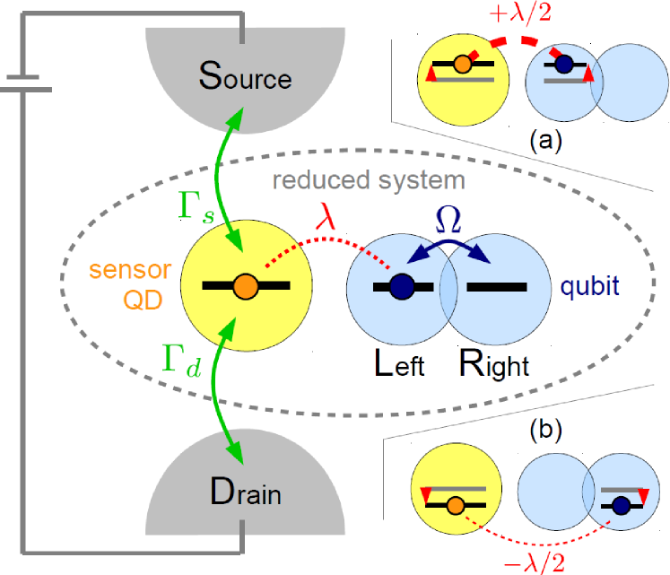
Figure 1: Sensor quantum dot (SQD) tunnel-coupled to source and drain electrode and capacitively coupled to a qubit, whose different logical states involve two possible positions left and right in a double quantum dot. If the qubit electron is left (a) or right (b), the Coulomb repulsion to the SQD electron is larger or smaller, respectively, compared to full delocalization of the qubit electron. We note that the spin-qubit readout can be mapped onto a charge-qubit readout utilizing spin-to-charge conversion.  

II Qubit readout

The readout of spin qubits is usually reduced to a charge readout by spin-to-charge conversion Elzerman et al. (2004); Barthel et al. (2010). Therefore, we focus here on the conceptually clearest problem, sketched in Fig. 1, namely the capacitive readout of a charge-qubit. The qubit itself consists of a double quantum dot occupied by a single electron, which occupies either an orbital localized on the left or right dot ($l=L,R$). These states are denoted by

$$|l\rangle = a_{l}^{{\dagger}}|0\rangle_{Q},$$ (1)

with $a_{l}$, $a_{l}^{{\dagger}}$ denoting the electron field operators of the qubit. The qubit is described by a Hamiltonian accounting for a real hopping amplitude $\Omega$ between the orbitals:

$$H_{Q} = \tfrac{1}{2}\Omega(a_{L}^{{\dagger}}a_{R}+a_{R}^{{\dagger}}a_{L}).$$ (2)

The isolated eigenstates of the qubit are thus superposition states $\tfrac{1}{\sqrt{2}}(a_{L}^{{\dagger}}\pm a_{R}^{{\dagger}})|0\rangle$, corresponding to an isospin in the $x$ direction when $a_{L}^{{\dagger}}|0\rangle$ and $a_{R}^{{\dagger}}|0\rangle$ denote isospin-up and -down along the $z$ direction, respectively. Since we assume that the real spin of the qubit electron does not couple to the measurement device, it remains fixed and we have omitted this quantum number from the beginning.

The sensor quantum dot (SQD) is modeled by a single, interacting, spin-degenerate orbital level with Hamiltonian

$$H_{S} = \sum_{\sigma}\varepsilon n_{\sigma}+Un_{\uparrow}n_{\downarrow},$$ (3)

containing the occupation operator $n_{\sigma}=d^{{\dagger}}_{\sigma}d_{\sigma}$ for electrons of spin $\sigma=\uparrow,\downarrow$, whose annihilation and creation operators are $d_{\sigma}$ and $d_{\sigma}^{{\dagger}}$, respectively. Due to the strong Coulomb repulsion of the quantum-confined electrons, the double occupation of the SQD costs an additional energy $U$. Typically, $U$ is the largest energy scale (except for the bandwidth of the leads, denoted by $D$): charging energies are on the order of $\sim 0.1-1$ meV Fujisawa et al. (2004); Lu et al. (2003b). Close to the SET resonance used for detection (cf. Sec. IV.1), this allows us to exclude the doubly occupied state of the SQD, retaining only $|0\rangle_{S}$ and $|\sigma\rangle_{S}=d_{\sigma}^{{\dagger}}|0\rangle_{S}$. This, however, implies that we need to keep track of the spin degree of freedom of the electrons (neglected in Ref. Gurvitz and Mozyrsky, 2008; Shnirman and Schön, 1998; Makhlin et al., 2001) unless a high magnetic field is applied. However, for singlet-triplet qubits the applied magnetic fields (required to define the qubit) are in the range of $\sim 100\mathrm{mT}$ Barthel et al. (2009); Petta et al. (2005). The corresponding energy splittings in GaAs are a few $\mu\mathrm{eV}$, which is much smaller than typical voltage bias $\sim 50\mu\mathrm{eV}$ Barthel et al. (2010). Therefore, both spin channels are energetically accessible and in general are relevant for the detection current through the SQD with noticeable consequences, as we discuss in Sec. IV.1. Furthermore, these magnetic energies are of the same order as typical tunneling rates $\Gamma$. This implies that renormalization effects may be important since states of the SQD plus qubit system can be mixed by the tunnel coupling to the electrodes. For the sake of simplicity, we assume zero magnetic field here, resulting in energy-degenerate spin-up and spin-down states on the SQD.

The readout of the qubit state using the SQD involves two couplings: the first one is the capacitive interaction of the total charge $n=n_{\uparrow}+n_{\downarrow}$ on the sensor QD with the charge configuration of the qubit, given by

$$H_{I} = \tfrac{1}{2}n\lambda(a_{L}^{{\dagger}}a_{L}-a_{R}^{{\dagger}}a_{R}).$$ (4)

This qubit-dependent energy shift by $\pm\lambda/2$ in turn affects the charge current through the SQD from the source to the drain electrodes, which are described as noninteracting reservoirs,

$$H_{R} = \sum_{r,k,\sigma}\omega_{rk\sigma}c^{{\dagger}}_{rk\sigma}c_{rk\sigma},$$ (5)

each in equilibrium at common temperature $T$, but held at different electrochemical potentials $\mu_{s}=V\text{/}2$ and $\mu_{d}=-V/2$. Here, $c_{rk\sigma}$ are the field operators referring to orbital $k$ and spin $\sigma$ in source ($r=s$) and drain ($r=d$), respectively. The second coupling involved in the readout process is the tunneling from the SQD to the electrodes, and vice versa, accounted for by

$$H_{T} = \sum_{r,k,\sigma}t_{r}c^{{\dagger}}_{rk\sigma}d_{\sigma}+\text{H.c.}.$$ (6)

The relevant energy scale is given, in terms of the tunneling amplitudes $t_{r}$ and the density of states $\nu_{r}$ of lead $r$, by the tunneling rates $\Gamma_{r}=2\pi|t_{r}|^{2}\nu_{r}$. For the sake of simplicity, we take both $t_{r}$ and $\nu_{r}$ to be spin $(\sigma)$ and energy $(k)$-independent. The source-drain coupling asymmetry $\gamma=\sqrt{\Gamma_{s}/\Gamma_{d}}$ of the SQD, however, is a crucial parameter.

For our analysis, we will assume the conceptually simplest continuous measurement limit $\lambda,\Omega\ll\Gamma$ and perform a controlled perturbative calculation. In the experimental situation Lu et al. (2003a); Barthel et al. (2010), in which the coupling $\lambda\sim\Gamma$, the effects may be even stronger.

III Charge-dependent isospin dynamics

III.1 Density operator and isospins

In the following, we express the action of the qubit state on the SQD and the corresponding backaction in terms of the isospin operator

$$\hat{\tau}_{i} = \sum_{l,l^{\prime}}(\sigma_{i})_{ll^{\prime}}a^{{\dagger}}_{l}a_{l^{\prime}},$$ (7)

where $\sigma_{i}$ denotes the Pauli matrix for $i=x,y,z$. The ensemble average of the isospin ${\bm{\tau}}=\langle\hat{{\bm{\tau}}}\rangle$ is obtained by averaging over the state of (integrating out) both electrodes and SQD. This qubit Bloch vector characterizes the reduced density operator of the qubit and is conveniently normalized to 1. Its $z$ component $\tau_{z}$ quantifies the imbalance of the probability to find the qubit electron in left orbital rather than the right orbital, while $\tau_{x}$ and $\tau_{y}$ quantify coherences between the left and right occupations.

It is, however, difficult to directly obtain a kinetic equation for the isospin ${\bm{\tau}}$ while incorporating the various effects of the measurement. A general reason for this is that the SQD is also a microscopic system, so that the action of the qubit on the sensor dynamics is not negligible, which then in turn affects the backaction of the sensor on the qubit. Another complication arises since we take into account an interacting detector (with proper spinful electrons), which technically can not be integrated out easily. Moreover, the SQD is driven out of equilibrium by the connected electron reservoirs.

We therefore instead derive a kinetic equation for the reduced density matrix $\rho(t)$ of SQD plus qubit by integrating out only the electrodes. Yet, this requires two Bloch vectors for a complete description of the qubit, as we now explain. The Hilbert space of the joint qubit-SQD system is spanned by six states denoted by $|\sigma\rangle_{S}\otimes|l\rangle_{Q}$ with $l=L,R$ referring to the state of the qubit and $\sigma=0,\uparrow,\downarrow$ denoting the state of the SQD. Thus, the reduced density operator $\rho(t)$ corresponds to a $6\times 6$ matrix. However, since the charge, the $z$ component of the (real) spin, and the total spin are conserved for the total system including the leads Leijnse and Wegewijs (2008), the reduced density operator is diagonal in the SQD degrees of freedom and independent of the choice of quantization axis of the real spin. Thus, we only need two $2\times 2$ density matrices $\rho^{n}_{Q}$, one for each of the two charge states of the SQD $n=0,1$:

$$\rho = \hat{P}^{0}\rho^{0}_{Q}+\hat{P}^{1}\rho^{1}_{Q}.$$ (8)

Here, $\hat{P}^{n}$ denotes the operator projecting onto the charge state $n=0,1$ of the SQD, that is,

$$\hat{P}^{0} = \text{}|0\rangle_{S}\text{}_{S}\langle 0|\otimes\mathbbm{1}_{Q},$$ (9)

$$\hat{P}^{1} = \sum_{\sigma=\uparrow,\downarrow}\text{}|\sigma\rangle_{S}\text{}_{S}\langle\sigma|\otimes\mathbbm{1}_{Q},$$ (10)

where $\mathbbm{1}_{Q}=\sum_{l}|l\rangle_{Q}\text{}_{Q}\langle l|$ is the qubit unit operator. Next, expanding each $\rho^{n}_{Q}$ in Eq. (8) in terms of the unit and three Pauli matrices, we find that the relevant part of the density operator is parametrized by only eight real expectation values $p^{n}=\mathrm{tr}(\hat{P}^{n}\rho)$ and $\tau^{n}_{i}=\mathrm{tr}(\hat{P}^{n}\hat{\tau}_{i}\rho)$:

$$\rho = \tfrac{1}{2}\sum_{n}p^{n}\hat{P}^{n}+\tfrac{1}{2}\sum_{n,i}\tau^{n}_{i}\left(\hat{P}^{n}\hat{\tau}_{i}\right).$$ (11)

The numbers $p^{n}=\mathrm{tr}(\hat{P}^{n}\rho)$ give the probability for the SQD to be in charge state $n=0$ or $1$. Probability conservation is expressed by

$$p^{0}+p^{1} = 1.$$ (12)

Furthermore, $\tau^{n}_{i}$ are the averages of the isospin components $i=x$, $y$, and $z$ when the SQD is in charge state $n=0$ or $1$, respectively. By definition these charge-projected isospins sum up to the average of the total isospin,

$${\bm{\tau}}^{0}+{\bm{\tau}}^{1} = {\bm{\tau}}.$$ (13)

III.2 Kinetic equations

The Hamiltonian of the isolated reduced system (qubit plus SQD with $H_{T}=0$) can be expressed in terms of the isospin operator as

$$H_{\text{red}} = \tfrac{1}{2}\mathbf{\Omega}\cdot\hat{{\bm{\tau}}}+\hat{P}^{1}\left(\varepsilon+\tfrac{1}{2}{\bm{\lambda}}\cdot\hat{{\bm{\tau}}}\right)$$ (14)

where the effective magnetic fields of the qubit mixing, $\mathbf{\Omega}=\Omega\mathbf{e}_{x}$, and the readout, ${\bm{\lambda}}=\lambda\mathbf{e}_{z}$, are orthogonal. Here we see the action of the measurement: the state of the qubit modulates the effective level position of the SQD between $\varepsilon\pm\lambda\text{/}2$. This affects the energy-dependent tunneling rates between the SQD and the leads and by this the measurable transport current.

The kinetic equations for the isolated reduced system, obtained from the von Neumann equation $\dot{\rho}=-i[H_{\mathrm{red}},\rho]$, show that the charge-projected isospins are subject to different, noncollinear effective magnetic fields $\mathbf{\Omega}$ and $\mathbf{\Omega}+{\bm{\lambda}}$:

$$\dot{p}^{0} = \dot{p}^{1}=0,$$ (15)

$$\dot{{\bm{\tau}}}^{0} = \mathbf{\Omega}\times{\bm{\tau}}^{0},$$ (16)

$$\dot{{\bm{\tau}}}^{1} = \left(\mathbf{\Omega}+{\bm{\lambda}}\right)\times{\bm{\tau}}^{1}.$$ (17)

If the SQD is singly occupied, the capacitive interaction ${\bm{\lambda}}$ thus exerts a backaction torque, perturbing the free qubit isospin precession about $\mathbf{\Omega}$.

We note that the ensuing analysis is, in general, not limited to charge qubits: For example, in singlet-triplet qubits, two exchange-coupled electrons in the qubit double quantum dot form spin-singlet and spin-triplet states, which due to a different charge distribution also couple capacitively to a sensor quantum dot (spin-to-charge conversion). However, the two-electron double quantum dot Hilbert space is four-dimensional instead of two-dimensional as for the charge qubit, which introduces an additional complexity to the problem that is beyond the scope of this paper. Still, as long as two electrons stay in the qubit subspace formed by the spin-singlet and the spin-triplet state $T_{0}$, the Hamiltonian (14) provides a valid model for the readout of a singlet-triplet qubit if one included a $z$ component into $\mathbf{\mathbf{\Omega}}$, accounting for the exchange splitting $J$ between $S$ and $T_{0}$ (the other two triplet states $T_{+}$ and $T_{-}$ are usually energetically split off by a large real magnetic field $B\gg J$). Note that the exchange interaction $J$ between the electrons is typically in the order of a few $\mu$eV Petta et al. (2005), which can be well below the tunneling rate $\Gamma$. This is a crucial requirement for our analysis.

When including the tunnel coupling $H_{T}$ of the SQD to the electronic reservoirs, Eqs. (15)–(17) turn into a set of equations that couple the occupation probabilities $p^{n}$ of the SQD and the charge-projected isospins $\tau^{n}$ ($n=0,1$). We derive these from the kinetic equation for the reduced density operator using the real-time diagrammatic technique Schoeller and Schön (1994); Schoeller (2009); Leijnse and Wegewijs (2008), including all coefficients of order $\Gamma$ as well as $\Gamma^{2}\text{/}T$, $\lambda\Gamma\text{/}T$, and $\Omega\Gamma\text{/}T$ and neglecting remaining terms of higher order in $\Gamma$, $\lambda$, and $\Omega$. In addition we make a Markov approximation. In Appendix A, we explain how to perform this expansion and justify its validity under the conditions $\lambda,\Omega\ll\Gamma\ll T$. Within these approximations the kinetic equations read as

$$\tfrac{d}{dt}\left(\begin{array}[]{c}p^{0}\\ p^{1}\\ {\bm{\tau}}^{0}\\ {\bm{\tau}}^{1}\end{array}\right) = \left(\begin{array}[]{cccc}-2\Gamma^{0}&+\Gamma^{1}&+2\mathbf{C}\cdot&+\mathbf{C}\cdot\\ +2\Gamma^{0}&-\Gamma^{1}&-2\mathbf{C}\cdot&-\mathbf{C}\cdot\\ +2\mathbf{C}&+\mathbf{C}&-2\Gamma^{0}+\left(\mathbf{\Omega}-2{\bm{\beta}}\right)\times&\Gamma^{1}-{\bm{\beta}}\text{}\times\\ -2\mathbf{C}&-\mathbf{C}&+2\Gamma^{0}+2{\bm{\beta}}\times&-\Gamma^{1}+\left(\mathbf{\Omega}+{\bm{\lambda}}+{\bm{\beta}}\right)\times\end{array}\right)\left(\begin{array}[]{c}p^{0}\\ p^{1}\\ {\bm{\tau}}^{0}\\ {\bm{\tau}}^{1}\end{array}\right).$$ (30)

When computing the matrix product with the column vector in the above equation, the dot “$\cdot$” (cross “$\times$”) in the entries of the matrix indicates that a three-dimensional scalar (vector) product is to be formed. The coefficients in  Eq. (30) are $\Gamma^{n}=\sum_{r=s,d}\Gamma^{n}_{r}$ with the renormalized dissipative SQD rates through junction $r=L,R$,

$$\Gamma^{0,1}_{r} = \Gamma_{r}f_{r}^{\pm}\pm\sum_{q=s,d}\tfrac{\Gamma_{r}\Gamma_{q}}{2T}(f^{+}_{r})^{\prime}\phi_{q}$$ (31)

$$\mp\sum_{q=s,d}\tfrac{\Gamma_{r}\Gamma_{q}}{2T}\phi^{\prime}_{r}(2f^{+}_{q}+f^{-}_{q}),$$

the vector $\mathbf{C}=\sum_{r}\mathbf{C}_{r}$ with the isospin-to-charge conversion rates

$$\mathbf{C}_{r} = \tfrac{\Gamma^{r}}{2T}{\bm{\lambda}}(-f_{r}^{+})^{\prime},$$ (32)

which are vectors with positive elements, and finally the vector ${\bm{\beta}}=\sum_{r}{\bm{\beta}}_{r}$, giving rise to isospin torque terms, with the effective magnetic fields

$${\bm{\beta}}_{r} = \tfrac{\Gamma_{r}}{T}\left(\mathbf{\Omega}+\tfrac{1}{2}{\bm{\lambda}}\right)\phi_{r}^{\prime}.$$ (33)

In Fig. 2, we plot the contribution of a single electrode to the magnitude of these coefficients as a function of the gate voltage $V_{g}$. In the above expressions $f^{\pm}_{r}=f^{\pm}((\varepsilon-\mu^{r})\text{/}T)$ abbreviates the Fermi function for lead $r=s,d$ with $f^{+}(x)=(e^{x}-1)^{-1}$ and $f^{-}(x)=1-f^{+}(x)$. The level renormalization function $\phi_{r}=\phi((\varepsilon-\mu^{r})\text{/}T)$ is defined by

$$\phi(x) = \mathcal{P}\int_{-\Lambda}^{+\Lambda}\frac{dy}{\pi}\frac{f^{+}(y)}{x-y}$$ (34)

$$= -\mathrm{Re}\text{ }\psi\left(\frac{1}{2}+i\frac{x}{2\pi}\right)+\ln\left(\frac{\Lambda}{2\pi}\right).$$ (35)

Derivatives are indicated by a dash: $\phi^{\prime}=\partial\phi(x)\text{/}\partial x$ and analogously $(f^{+})^{\prime}=\partial f^{+}(x)\text{/}\partial x$. In Eq. (34), $\mathcal{P}$ denotes the principal value of the integral with a cutoff $\Lambda=D\text{/}T$, yielding the real part of the digamma function $\psi$ and a logarithmic correction. The latter depends on the electrode bandwidth $D$, which must be set to $D\sim U$ where $U$ is the large local Coulomb interaction energy of the SQD (we excluded the doubly occupied state from the SQD Hilbert space). In this way $D\sim U$ enters into the rates, Eq. (31), but $D$ drops out in the derivatives required for the torque terms, Eq. (33). Finally, although we refer to Eq. (31) simply as the “renormalized” SQD rate, one should note that the $O(\Gamma^{2})$ corrections to the $O(\Gamma)$ rate (first term) includes both renormalization of the energy level $\varepsilon$ (second term) as well as an elastic cotunneling contribution (third term). Fig. 2(a) shows that this leads to a combined shift and broadening of the resonant step in the rates around $\varepsilon\approx\mu_{r}$; cf. Appendix C. We note that we were careful to restrict our study to weak couplings $\Gamma\ll T$. This clearly validates the neglect of even higher-order corrections. In particular, we can safely exclude the occurrence of Kondo physics even for those results we show in the Coulomb blockade regime.

Figure 2: Dissipative and coherent coefficients induced by a single electrode for $\mu=0$ (electrode index suppressed for simplicity). (a) Dissipative SQD rates $\Gamma^{0,1}$ (31) including the renormalization of the tunneling (solid lines) and excluding it (dashed lines) as a function of gate voltage $V_{g}=-\varepsilon$. Parameters: $\Gamma\text{/}T=0.2$ and $D/T=10^{2}$. (b) $z$ component of the isospin-to-charge conversion rate $C_{z}$,  Eq. (32), (blue) and the isospin torque $\beta_{z}$, Eq. (33), (red) as a function of $V_{g}$. Since $\Omega_{z}=0$ the curve with the scaling chosen is independent of further parameters. Note that the $C_{z}$ drops exponentially in the Coulomb blockade regime, whereas $\beta_{z}$ decreases only algebraically.

III.3 Sum rules

The kinetic equations (30) clearly satisfy the sum rule $\dot{p}^{0}+\dot{p}^{1}=0$, which expresses the probability conservation, Eq. (12). Moreover, we discuss in Appendix D that a second sum rule exists for the charge-projected isospins: their sum has to reproduce the internal evolution of the total average isospin, i.e. as if the tunneling was switched off ($H_{T}=0$); see also Ref. Salmilehto et al., 2012. Their sum is thus given by Eqs. (16) and (17):

$$\dot{{\bm{\tau}}}^{0}+\dot{{\bm{\tau}}}^{1} = \dot{{\bm{\tau}}}|_{\text{int}}=\mathbf{\Omega}\times\left({\bm{\tau}}^{0}+{\bm{\tau}}^{1}\right)+{\bm{\lambda}}\times{\bm{\tau}}^{1}.$$ (36)

This constrains the dynamics of the average charge-projected isospins ${\bm{\tau}}^{0}$ and ${\bm{\tau}}^{1}$, without reducing one to the other (as happens for $p^{0}$ and $p^{1}$). The isospin sum rule is a consequence of the conservation of the total isospin operator in the tunneling, that is, $\left[\hat{{\bm{\tau}}},H_{T}\right]=0$ Salmilehto et al. (2012). It holds in the presence of the reservoirs, order-by-order in the perturbation expansion in $\Gamma$. Indeed, we find that our kinetic equations obey Eq. (36), as do the results in Ref. Makhlin et al., 2001. By contrast, Eqs. (31a)-(31f) given in Ref. Gurvitz and Mozyrsky, 2008 in general violate it, unless one expands to lowest order in the SQD-qubit coupling $\lambda$. In that case, assuming energy-dependent tunneling rates, they agree with our kinetic equations if we (i) send the bias to infinity, implying energy-independent Fermi functions $f_{L}^{+}=f_{R}^{-}=1$ and $f_{L}^{-}=f_{R}^{+}=0$ in Eq. (30), (ii) neglect all renormalization effects, i.e., the isospin torque and the renormalization of the tunneling rates, and (iii) ignore factors of two due to the SQD spin (importance discussed in Sec. IV.1).

III.4 Isospin torques

The kinetic equations (30) together with the probability conservation $p^{0}+p^{1}=1$ completely determine the Markovian dynamics of the reduced SQD-qubit system in the limit $\lambda,\Omega\ll\Gamma\ll T$. The dynamics of the occupations and the isospins are coupled by the charge-to-isospin conversion vector rates $\mathbf{C}$: in the first line of Eq. (30), they describe the influence of the qubit state on the occupations, that is, the measurement action, which modifies the current, whereas in the second and third lines of Eq. (30), they represent a backaction of the measurement on the qubit. These dissipative terms scale as $\sim\Gamma\lambda\text{/}T$, i.e., with the product of both couplings that are involved in the measurement process.

When keeping the above terms $\mathbf{C}\sim\Gamma\lambda\text{/}T$ that describe the readout action and backaction, we must also keep torque terms ${\bm{\beta}}\times{\bm{\tau}}^{n}$ induced by the readout since ${\bm{\beta}}$ scales in the same way (since $\lambda\sim\Omega$ or even $\lambda<\Omega$) unless prefactors are very small. These torque terms represent a coherent backaction on the qubit since it derives from level renormalization effects. The isospin torque terms have a nontrivial voltage dependence. At the resonance of the SQD level with the electrochemical potential $\mu_{r}$, $\varepsilon=-V_{g}=\mu_{r}$, the effective magnetic field from lead $r$ vanishes, $|{\bm{\beta}}_{r}|=0$. However, it sharply rises to two extrema at $|\varepsilon-\mu_{r}|\approx 2T$, i.e., at the “flanks” of the Coulomb peaks. Figure 2(b) shows that here $|{\bm{\beta}}|\sim|\mathbf{C}|$, right at the crossover regime from single electron tunneling to Coulomb blockade where the SQD has the highest readout sensitivity. Further away from resonance the dissipative (back)action terms ($\mathbf{C}$) are exponentially suppressed with $|\varepsilon-\mu_{r}|$, so that the torque terms even start to dominate: the field ${\bm{\beta}}$ only decays algebraically with $\phi^{\prime}_{r}\sim 1\text{/$|\varepsilon-\mu_{r}|$}$. The latter approximation holds when the bias is the largest energy scale.

It is explicitly stated in Ref. Makhlin et al., 2001; Shnirman and Schön, 1998 that level renormalization contributions are neglected. In the limit of infinite bias $V_{b}$ torque effects can be neglected as done in Refs. Gurvitz and Berman, 2005; Gurvitz and Mozyrsky, 2008 because the magnitude of ${\bm{\beta}}$ scales as $\left|{\bm{\beta}}\right|\sim 1\text{/}V_{b}$. Thus, our results agree in this regard with Refs. Gurvitz and Berman, 2005; Gurvitz and Mozyrsky, 2008. Altogether, it is therefore not surprising that the coherent backaction has not been noted so far. However, if the bias $V_{b}$ is large, but finite, corrections from renormalization effect can still be sizable, see also Ref. Wunsch et al., 2005 for a related discussion. Thus, one should also reckon with renormalization effects when suppressing the readout current by tuning the SQD into Coulomb blockade where the qubit state is supposed not to be measured (during other processing steps, e.g., qubit manipulation). Although this nearly eliminates the dissipative backaction ($\left|\mathbf{C}\right|\approx 0$), the coherent backaction may still be of appreciable size. Thus, this nontrivial dependence of the induced torque on the gate (and bias) voltage, illustrated in Fig. 2(b), presents interesting possibilities that may be used to control the quantum state of a qubit.

We finally discuss the relaxation rates $\sim\Gamma+\Gamma^{2}\text{/}T$ [Eq. (31)]: they only contain the tunneling, i.e., they are associated with the stochastic switching of the detector. Clearly, when describing the readout for $\lambda\lesssim\Gamma$ one has to consistently include the renormalization of the tunneling rates $\sim\Gamma^{2}\text{/}T$ [second and third term in Eq. (31)]. To our knowledge, this has not been pointed out so far (cf. Ref. Gurvitz and Berman, 2005; Gurvitz and Mozyrsky, 2008; Shnirman and Schön, 1998; Makhlin et al., 2001). In Appendix B, we show that this consistency is mandatory to obtain physically meaningful results: when failing to account for the next-to leading order terms $\sim\Gamma^{2}\text{/}T$, while keeping the coherent backaction effects (isospin torques), the solution of the above kinetic equations may severely violate the positivity of the density matrix (11).

III.5 Analogy to quantum-dot spin-valves

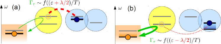
Figure 3: Illustration of coherent processes responsible for the torque terms $\sim{\bm{\beta}}$ in Eq. (30) for $\Omega=0$ (for further explanation, see Sec. III.5).

The torque terms in Eq. (30) are generated by coherent fluctuations of electrons tunneling between the SQD and the leads. A similar coherent effect is well-known in spintronics:Braun et al. (2004); J. König and J. Martinek (2003) when attaching a quantum dot to ferromagnetic leads, an imbalance of the tunneling rates for spin-up and spin-down electrons leads to a different level shift for the spin-up state and the spin-down state on the quantum dot. The resulting level splitting shows up as an additional spin torque proportional to $\phi(\varepsilon)$ [see Eq. (34)] in the kinetic equations resembling our qubit isospin equations.Braun et al. (2004) In analogy to this case, here the strength of the virtual fluctuations of the SQD depends on the position of the electron in the qubit (see Fig. 3). For the special case $\Omega=0$ a simple argument can be made: if the isospin is up (down), the effective level position of the qubit is shifted by $+\lambda\text{/}2$ ($-\lambda\text{/}2$). This gives a level splitting $\sim\phi_{r}\left(\tfrac{1}{T}(\varepsilon+\tfrac{\lambda}{2})\right)-\phi_{r}\left(\tfrac{1}{T}(\varepsilon-\tfrac{\lambda}{2})\right)\approx\tfrac{\lambda}{T}\phi^{\prime}_{r}(\varepsilon)$ in the weak coupling limit and explains why Eq. (33) contains a derivative of the renormalization function. [The factor 1/2 in Eq. (33) occurs because the isospin operator is not normalized.] For nonzero mixing $\Omega$ of the qubit orbitals the additional vector $\sim\tfrac{\mathbf{\Omega}}{T}\phi^{\prime}_{r}(\varepsilon)$ appears in Eq. (33) along a different direction. This accounts for a renormalization of the qubit splitting.

These torque terms act on the charge-projected isospins, but for the different charge sectors they have opposite directions [as required by the sum rule (36)] and differ in strength by a factor of 2 (due to the SQD electron spin):

$$\dot{{\bm{\tau}}}^{0} = \left(\mathbf{\Omega}-2{\bm{\beta}}\right)\times{\bm{\tau}}^{0}-{\bm{\beta}}\text{}\times{\bm{\tau}}^{1}+\ldots,$$ (37)

$$\dot{{\bm{\tau}}}^{1} = 2{\bm{\beta}}\times{\bm{\tau}}^{0}+\left(\mathbf{\Omega}+{\bm{\lambda}}+{\bm{\beta}}\right)\times{\bm{\tau}}^{1}+\ldots.$$ (38)

As in kinetic equations for QD spin valves with nonzero spin in two adjacent charge states Baumgärtel et al. (2011), in Eq. (37)-(38) we have a spin torque that precesses the isospin ($\dot{{\bm{\tau}}}^{0}\sim-2{\bm{\beta}}\times{\bm{\tau}}^{0}$ and $\dot{{\bm{\tau}}}^{1}\sim{\bm{\beta}}\times{\bm{\tau}}^{1}$). However, in contrast to the spin-valve equations, their sign is opposite for $n=0$ and $n=1$. Additionally, there are torque terms that couple the two isospins of different charge states of the SQD ($\dot{{\bm{\tau}}}^{0}\sim-{\bm{\beta}}\times{\bm{\tau}}^{1}$ and $\dot{{\bm{\tau}}}^{1}\sim 2{\bm{\beta}}\times{\bm{\tau}}^{0}$). Those turn out to be crucial as we explain in the next section.

IV Impact of coherent backaction

IV.1 Readout current

By taking the SQD spin and the strong local interaction $U$ on the SQD into account, the dissipative rates involving $p^{0}$ and ${\bm{\tau}}^{0}$ in our kinetic equations (30) differ from Ref. Gurvitz and Berman, 2005; Gurvitz and Mozyrsky, 2008; Shnirman and Schön, 1998; Makhlin et al., 2001 by a factor of 2, as expected. A less obvious, but important difference arises for the qubit-dependent part of the current flowing through the SQD, i.e., the difference of the current for finite coupling $(I_{\lambda})$ and zero coupling $(I_{0})$

$$\Delta I := I_{\lambda}-I_{0}.$$ (39)

In the stationary limit ($\dot{p}^{n}=0$, $\dot{{\bm{\tau}}}^{n}=0$) $\Delta I$ may be expressed as

$$\Delta I = (\Gamma^{0}_{s}-\Gamma^{0}_{d})(p^{0}_{\lambda}-p^{0}_{0})-\tfrac{1}{2}(\Gamma^{1}_{s}-\Gamma^{1}_{d})(p^{1}_{\lambda}-p^{1}_{0})$$ (40)

$$-\tfrac{1}{2}\left(\mathbf{C}_{s}-\mathbf{C}_{d}\right)\cdot\left(2{\bm{\tau}}^{0}_{\lambda}+{\bm{\tau}}^{1}_{\lambda}\right).$$

where $p^{n}_{\lambda}$, ${\bm{\tau}}^{n}_{\lambda}$ and $p^{n}_{0}$, ${\bm{\tau}}^{n}_{0}$ are the stationary solutions of Eq. (30) for finite and zero coupling $\lambda$, respectively. Although we will refer to $\Delta I$ as the “signal current”, Eq. (40) reveals it will in general not directly measure the position of qubit electron for two reasons. First, the SQD occupations $p^{n}_{\lambda}$ depend on the isospins through the kinetic equations [see Eq. (30)]: the last term term in Eq. (40), the one explicitly depending on the ${\bm{\tau}}^{n}_{\lambda}$, is not the only contribution to $\Delta I$. Secondly, even this latter term is not directly sensitive to the total isospin ${\bm{\tau}}={\bm{\tau}}^{0}+{\bm{\tau}}^{1}$ since ${\bm{\tau}}^{0}$ is weighted with the factor of 2 (due to the SQD-spin degeneracy) relative to ${\bm{\tau}}^{1}$ in Eq. (40).

We now study the impact of the torque terms ${\bm{\beta}}\times{\bm{\tau}}^{n}$ in Eq. (30) on the signal current $\Delta I$. Solving (30) in the stationary limit and inserting it into Eq. (40) yields, to leading orders of $\lambda$ and $\Omega$,

$$\Delta I_{\beta=0} = \frac{\left|\mathbf{C}\right|^{2}}{\Gamma^{1}}\frac{\Gamma^{0}+\Gamma^{1}}{2\Gamma^{0}+\Gamma^{1}}\left[\frac{\left|\mathbf{C}_{s}\right|}{\left|\mathbf{C}\right|}-\frac{2\Gamma^{0}_{s}+\Gamma^{1}_{s}}{2\Gamma^{0}+\Gamma^{1}}\right],$$ (41)

$$\frac{\Delta I_{\beta\neq 0}}{\Delta I_{\beta=0}} = 1+\frac{\kappa(\Gamma^{0}\text{/}\Gamma^{1}-\Gamma^{1}\text{/}\Gamma^{0})}{1-\kappa\text{/}2(1-\Gamma^{1}\text{/}\Gamma^{0}+2\Gamma^{0}\text{/}\Gamma^{1})},$$ (42)

with $\kappa=\sum_{r}\left(\Gamma_{r}\text{$\phi^{\prime}_{r}$/}T\right)$. At least to lowest order, Eqs. (41) and (42) are independent of $\Omega$ [explained below Eq. (44)]. The signal currents (41) and (42) are plotted in Fig. 4(a); let us first focus on their main features. To this end we neglect the change in the occupations of the SQD due to the coupling to the qubit: setting $p^{n}_{\lambda}=p_{0}^{n}$ in Eq. (40) we obtain, for symmetric tunnel couplings,

$$\Delta I \approx \tfrac{\Gamma\lambda}{4T}[(f_{s}^{+})^{\prime}-(f_{d}^{+})^{\prime}](2\tau^{0}_{z}+\tau^{1}_{z}).$$ (43)

In this case, a nonzero isospin polarization acts as an additional gate voltage on the SQD and shifts the effective level position in the SQD to $\varepsilon+\lambda\tau^{z}\text{/}2$ [see Eq. (14)]. The signal current (40) is then just the linear response of the tunneling rates $\Gamma_{r}^{n}(\varepsilon)\rightarrow\Gamma_{r}^{n}(\varepsilon+\lambda\tau^{z}\text{/}2)$ to that shift. In our case, the energy dependence of these rates (31) is mostly through the Fermi functions, which change sharply when the level is aligned with the electrochemical potentials of source and drain. This explains the s-shaped curve with a maximum / minimum roughly expected at $V_{g}\approx\mp V_{b}\text{/}2$, which is in fact slightly shifted towards the adjacent Coulomb blockade regimes (see Fig. 4) since $\tau^{z}$ still increases on the threshold to Coulomb blockade.

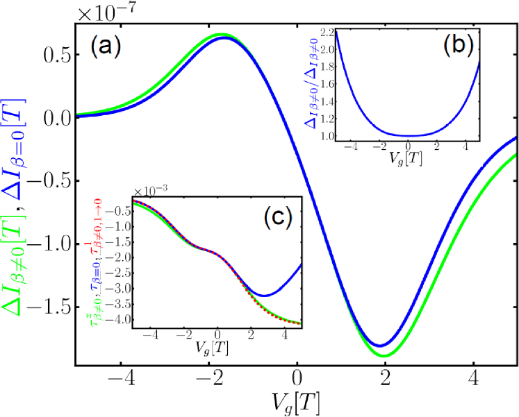
Figure 4: (a, main panel) Signal current including torque terms (green) and excluding torque terms (blue), and (b) the ratio of these two currents as a function of gate voltage $V_{g}$. (c) $z$ component of the total isospin ${\bm{\tau}}={\bm{\tau}}^{0}+{\bm{\tau}}^{1}$ including torque terms (green), excluding torque terms (blue) and the $z$ component of charge-projected isospin ${\bm{\tau}}^{1}$ when we only keep the term $\dot{{\bm{\tau}}}^{0}=-{\bm{\beta}}\times{\bm{\tau}}^{1}$ in Eq. (30) (dashed red). In (a)-(c) the remaining parameters are the same: $V_{b}\text{/}T=3$, $\Gamma^{L}\text{/}T=\Gamma^{R}\text{/}T=10^{-1}$, $\lambda\text{/}T=10^{-2}$, and $D/T=10^{3}$.

The second feature of Fig. 4(a) is the notable asymmetry of the s-shaped curve: the amplitude of the signal is larger for positive than for negative gate voltages, which we explain in the following. To this end, we now first neglect the torque terms in Eq. (30). The stationary solution of the resulting equations shows that the charge-projected isospins relax until they are antiparallel to the effective field in that charge sector (the reduced system tends to occupy the ground state), that is,

$$\begin{array}[]{lllllll}{\bm{\tau}}^{0}_{\beta=0}&=&-c^{0}\mathbf{\Omega},&&{\bm{\tau}}^{1}_{\beta=0}&=&-c^{1}\left(\mathbf{\Omega}+{\bm{\lambda}}\right),\end{array}$$ (44)

with $c^{0},c^{1}>0$. Clearly, only ${\bm{\tau}}^{1}_{\beta=0}$ has a component along the detection vector ${\bm{\lambda}}$ and it therefore solely determines  the signal in the case of ${\bm{\beta}}=0$ by Eq. (43). When the gate voltage is lowered, the SQD is more likely to be empty and ${\bm{\tau}}^{1}_{\beta=0}$ is suppressed. This is evident from the kinetic equations (30) since the relaxation rate $\Gamma^{1}$ of ${\bm{\tau}}^{1}_{\beta=0}$ rises while the relaxation rate $\Gamma^{0}$ of ${\bm{\tau}}^{0}_{\beta=0}$ becomes smaller when $V_{g}$ is lowered, thus transferring a nonzero total isospin to the projection ${\bm{\tau}}^{0}_{\beta=0}$ rather than to ${\bm{\tau}}^{1}_{\beta=0}$. In conclusion, the signal has the overall tendency to be decreased with $V_{g}$, explaining the asymmetry of the maximum and minimum magnitudes. Finally, one understands why the signal is independent of $\Omega$: the coefficient $c_{1}$, relevant for the signal, is determined exclusively by the relaxation (31) and isospin-to-charge conversion rates (32), which do not depend on $\Omega$. This independence of $\Omega$ is maintained even when torque terms are then included because corrections to the solution for ${\bm{\beta}}=0$ are of higher order in $\lambda$ and $\Omega$ and are thus disregarded in Eqs. (41) and (42), except for those coming from the torque terms along ${\bm{\lambda}}$.

Comparing the two curves in Fig. 4(a) we note that the impact of the torque terms on the signal current become quite significant. Remarkably, the isospin-torque correction to the signal current may be of the same order as the signal current itself when entering the Coulomb blockade regime. In Fig. 4(b) we plot the ratio $\Delta I_{\beta\neq 0}\text{/}\Delta I_{\beta=0}$, which can achieve values even as large as 2 for the parameters chosen. The reason for this may be inferred from Eq. (42): when tuning away from resonance in either direction, $|\phi^{\prime}|$ and therefore $\kappa$ in Eq. (42) quickly reaches a maximum [see Fig. 2(b)] and simultaneously either $\Gamma^{0}\text{/}\Gamma^{1}$ or $\Gamma^{1}\text{/}\Gamma^{0}$ rises [see Fig. 2(a)]. Beyond the maximum the latter effect dominates, sustaining a further increase of the ratio $\Delta I_{\beta\neq 0}\text{/}\Delta I_{\beta=0}$.

To identify which terms in the kinetic equations (30) are responsible for this correction, we compare in Fig. 4(c) the $z$ component of the total isospin ${\bm{\tau}}$ when torque terms are included with the $z$ component of ${\bm{\tau}}^{1}$ for the case when we only keep the term $\dot{{\bm{\tau}}}^{0}\sim-{\bm{\beta}}\times{\bm{\tau}}^{1}$ in Eq. (30). Clearly, this term is sufficient to reproduce the total isospin polarization for $V_{g}>0$. The above suggests that the torque-induced isospin polarization is the result of a two-step mechanism: first, a charge transition from $n=1$ to $n=0$ occurs in the SQD, accompanied by an induced coherent precession with frequency $\left|{\bm{\beta}}\right|$ of the isospin. After that, a dissipative transition to charge state $n=0$ takes place with rate $\Gamma^{0}$. By these two steps, the isospin ${\bm{\tau}}^{1}$ experiences effectively the effective magnetic field  $\mathbf{B}^{0}=\mathbf{\Omega}+{\bm{\lambda}}$ [due to $\dot{{\bm{\tau}}}^{1}\sim\left(\mathbf{\Omega}+{\bm{\lambda}}\right)\times{\bm{\tau}}^{1}$] plus an additional, noncollinear contribution along $-{\bm{\beta}}$ (due to $\dot{{\bm{\tau}}}^{0}\sim-{\bm{\beta}}\times{\bm{\tau}}^{1}$). We checked that the torque term $\dot{{\bm{\tau}}}^{1}\sim{\bm{\beta}}\times{\bm{\tau}}^{1}$ in Eq. (30) is not important here by simply leaving it out. Thus, the total effective field $\mathbf{B}^{0}-{\bm{\beta}}$ is slightly rotated towards $+{\bm{\lambda}}$ if $\phi^{\prime}>0$ (as for positive $V_{g}$, cf. Fig. 2) as compared to $\mathbf{B}^{0}$. Since ${\bm{\tau}}^{1}$ tends to orient itself antiparallel to these effective magnetic fields, it acquires a component along $-{\bm{\lambda}}$, resulting in a decrease in $\tau_{z}$ [cf. Fig. 4(c)]. A similar analysis shows that for negative $V_{g}$ the dominant effect comes rather from the charge-state-conserving torque term $\dot{{\bm{\tau}}}^{0}={\bm{\beta}}\times{\bm{\tau}}^{0}$ in Eq. (30).

IV.2 Differential readout conductance

We next discuss the differential signal conductance

$$\Delta G = \frac{\partial\Delta I}{\partial V},$$ (45)

which is directly measured in experiments Barthel et al. (2010). Our findings are summarized in Fig. 5, which compares $\Delta G\sim\lambda^{2}\Gamma\text{/}T^{3}$, plotted as a function of gate voltage when including and excluding the torque terms, as well as their difference, the torque correction $\delta G=\Delta G_{\beta\neq 0}-\Delta G_{\beta=0}\sim\lambda^{2}\Gamma\text{/}T^{3}\kappa\sim\lambda^{2}\Gamma^{2}/T^{4}$. Figures 5(a) and (c) corroborate that the relative impact of the torque terms on the conductance signal, $\delta G\text{/}\Delta G\sim\kappa$, becomes larger when $\kappa\sim\Gamma\text{/}T$ is increased. This is generally expected for renormalization effects. Fig. 5(c) illustrates that an asymmetry of tunnel rates $\gamma=\sqrt{\Gamma^{s}\text{/}\Gamma^{d}}>1$ enhances the torque effects as well. This is also expected, since in this case the SQD is emptied less often than it is filled, leaving it nearly always singly occupied. Then the coupled SQD-qubit undergoes long periods of coherent time evolution and the torque terms can precess the isospin more effectively than for the opposite asymmetry $\gamma\leqslant 1$.

Figure 5: Differential signal conductance  (45) at finite bias $V_{b}=3T$ as a function of gate voltage $V_{g}=-\varepsilon$. In all plots, we set $D\text{/}T=10^{3}$. $\Delta G$ is shown both including torque terms (green) and neglecting them (blue) in (a,c) and their difference $\delta G$ is shown in (b,d). In (a,b) we compare the results for coupling strengths, $\Gamma^{s}\text{/}T=\Gamma^{d}\text{$\text{/}$}T=10^{-f}$ and $\lambda\text{/}T=10^{-2f}$ for symmetric tunnel rates $\gamma=1$, while in (b,d) we change the tunnel couplings asymmetry $\gamma=\sqrt{\Gamma^{s}\text{/}\Gamma^{d}}$ while keeping $\sqrt{\Gamma^{s}\Gamma^{d}}\text{/}T=5\cdot 10^{-2}$ and $\lambda\text{/}T=10^{-3}$ fixed. The curves in (a), (c), and (d) are vertically offset for different parameters with the $\Delta G\text{/}\delta G=0$ line indicated by the gray dotted lines. The axis labels refer to the lowest curve. Note the units in (a) and (b), which account for the scaling of the conductance signal $\Delta G\sim\lambda^{2}\Gamma\text{/}T^{3}$.

In Fig. 6 we systematically investigate the impact on the two main features of the $\Delta G$ traces of Fig. 5(a,b), namely the position and its magnitude of the large dip at $V_{g}>0$. We plot the absolute correction due to the isospin torque to the dip position

$$\delta V_{g}^{\mathrm{dip}} = V_{g,\beta\neq 0}^{\mathrm{dip}}-V^{\mathrm{dip}}_{g,\beta=0},$$ (46)

and a relative correction to its magnitude,

$$R = \frac{\Delta G^{\mathrm{dip}}_{\beta\neq 0}-\Delta G^{\mathrm{dip}}_{\beta=0}}{\Delta G^{\mathrm{dip}}_{\beta=0}},$$ (47)

as a functions of the bias voltage. In Fig. 6(a,b) we see $\delta V_{g}>0$ for all biases and parameters, i.e., the dip is shifted deeper into the Coulomb blockade regime due to the isospin torque. As expected from the above discussion of Fig. 5, the correction to the position increases when $\Gamma/T$ rises as in Fig. 6(a) or the asymmetry  $\Gamma^{s}>\Gamma^{d}$ rises as in Fig. 6(b).

By contrast, Fig. 6(c) shows that the qualitative correction $R$ to the magnitude depends on the parameters: for small bias, the dip is enhanced $(R>0)$ by the torque terms, while it is suppressed  $(R<0)$ in the limit of large bias. Figure 6(d) shows that this tendency is independent of the asymmetry of the tunnel couplings. If the source tunneling barrier is more transparent $(\Gamma^{s}>\Gamma^{d})$, we find a nonmonotonic dependence with a strong enhancement of the dip close to $V_{b}\sim 2T$ that can reach up to 30% for an asymmetry of $\Gamma^{s}\text{/}\Gamma^{d}=9$, a typical experimental value. In this case the dip position correction $\delta V_{g}$ in Fig. 6(b) is also nonmonotonic. Again this corroborates the increased relative importance of the torque terms due to long waiting times in the SQD.

Figure 6: Bias dependence of the torque corrections. The correction $\delta V_{g}^{\mathrm{dip}}$, given by Eq. (46), is shown in (a) for different coupling strengths $\Gamma^{s}\text{/}T=\Gamma^{d}\text{$\text{/}$}T=\sqrt{\lambda\text{/}T}=10^{-f}$ and in (b) for different asymmetries $\gamma=\sqrt{\Gamma^{s}\text{/}\Gamma^{d}}\text{}$. The relative correction $R$, given by Eq. (47), is shown in (c) for different couplings and in (d) for different asymmetries, chosen as in (a) and (b), respectively. All definitions and other parameters are the same as in Figs. 5(a) and (b).

V Summary and Outlook

We have analyzed the backaction of a capacitive readout of a charge qubit by probing the differential conductance of a nearby sensor quantum dot (SQD). To this end we extended the kinetic equations used previously Gurvitz and Berman (2005); Gurvitz and Mozyrsky (2008); Shnirman and Schön (1998); Makhlin et al. (2001) by including spin, local interaction on the SQD and, most importantly, renormalization effects of (i) the level positions of the coupled SQD-qubit system, generating qubit-isospin torques and (ii) the tunneling rates connecting the SQD to the electrodes. Our study, focused on the ensemble-averaged, stationary conductance signal, already provides indications that these renormalization effects are important for such detection schemes. In particular, at the crossover to Coulomb blockade (the experimentally relevant regime of highest detection sensitivity), these effects matter.

The isospin torque terms $\sim{\bm{\beta}}\times{\bm{\tau}}^{n}$ in the kinetic equations for the coupled SQD-qubit system induce an additional precession of charge-projected qubit isospins ${\bm{\tau}}^{n}$. This renormalization effect relies on the response of the SQD tunneling rate – scaling as $\sim\Gamma$ – to perturbations on the internal energy scales $\sim\Omega,\lambda$ of the SQD-qubit system. This is exactly the sensitivity that is also exploited for the readout of the qubit state. Thus, isospin torques cannot be avoided since they incorporate terms that scale in the same way with these parameters as the terms responsible for the readout.

We have compared these isospin torque terms with analogous terms due to the spintronic exchange field that is found in quantum dot spin valves J. König and J. Martinek (2003); Martinek et al. (2003); Hauptmann et al. (2008); Gaass et al. (2011). In the latter, the spin-dependent level renormalization that the field represents is caused by spin-dependent tunneling rates, while the above qubit-torque terms derive from an isospin-dependent effective level position of the electron in the SQD that is used in the readout. A consequence of this difference in the microscopic origin is that the isospin torque can additionally couple isospins for different SQD charge states ($n=0,1$), e.g., terms such as  $\dot{{\bm{\tau}}}^{1}\sim{\bm{\beta}}\times{\bm{\tau}}^{0}$ appear, in addition to a precession that preserves this charge state, i.e., terms of the form $\dot{{\bm{\tau}}}^{n}\sim{\bm{\beta}}\times{\bm{\tau}}^{n}$. The latter are the only ones that appear in spintronics. We discussed that both types of isospin torque terms are crucial for the description of the stationary readout.

Furthermore, the renormalization of the SQD detector tunnel rates (level shifts and cotunneling) is found to be crucial: without those terms, the positivity of the density operator can be severely violated, invalidating the approach, at least in the Markovian limit (see Appendix B). These corrections, extensively studied in transport through QDs, have so far received little attention in the context of quantum measurements  and require one to go beyond the standard Born-Markov approximation plus secular approximation. We have provided an important, general check on any such extension by deriving a rigorous sum rule for the charge-projected isospins that holds order-by-order in the SQD tunnel coupling $\Gamma$. This sum rule, recently discussed in a general setting Salmilehto et al. (2012), is imposed by the conservation of the qubit isospin during tunneling and in fact holds for any qubit-SQD observable that respects this symmetry.

The basic reason why renormalization effects are important in weak measurements is a simple one: if an electron on the detector quantum dot has time to probe the qubit, it also has time to fluctuate and thereby renormalize system parameters. For the parameter regime considered here, $\Omega,\lambda\lesssim\Gamma$, standard Born-Markov approximations, combined with Davies’ secular approximation, are not applicable, as we have explicitly verified, and these furthermore violate the above general sum rule.

The kinetic equations presented here provide a new starting point for studying the impact of the isospin torque on the transient dynamics of the qubit Bloch vector and the measurement dynamics. The measurement-induced isospin torques lead to a modification of the relaxation and dephasing rates of the isospin $\mathbf{\tau}=\mathbf{\tau}^{0}+\mathbf{\tau}^{1}$, which can be found by solving the kinetic equations (30) time-dependently for a given initial state. Preliminary results indicate that the time for the exponential decay of the isospin magnitude $\left|\mathbf{\tau}\right|$ to its stationary value can be significantly altered. However, the study of such transient effects requires the non-Markovian corrections into Eq. (30). Here an interesting question is the possible additional rotation of the qubit Bloch vector due to the torque terms during the decay. Thus, the coherent backaction may not only be a nuisance, but could also be useful for the manipulation of qubits due to the electric tunability of the isospin torques that we derived here. More generally, the analogy of charge readout in quantum information processing with spintronics of quantum dot devices may be a fruitful one to be explored further.

Appendix A Real Time Diagrammatics

We derive the kinetic equations (30) for the averages occurring in Eq. (11) by applying the real-time diagrammatic technique, Schoeller and Schön (1994); Schoeller (2009); Leijnse and Wegewijs (2008) which we briefly review here to introduce the notation and to give the starting point for the discussion of the approximations we employ. The real-time diagrammatic technique starts from the von-Neumann equation for the density operator of the total system,

$$\dot{\rho}_{\text{tot}}(t) = -iL\rho_{\text{tot}}(t)-i(L_{T}+L_{R})\rho_{\text{tot}}(t),$$ (48)

with the Liouvillians $L_{\alpha}\cdot=\left[H_{\alpha},\text{ $\cdot$ }\right]$ for $\alpha=Q,R,S,T,I$ and $L=L_{Q}+L_{S}+L_{I}$ mediating the free evolution of SQD and qubit (cf. Sec. II). Here, the dot “$\cdot$” indicates the operator on which the superoperator $L_{\alpha}$ acts. Assuming a factorizable initial state $\rho_{\text{tot}}(t_{0})=\rho(t_{0})\otimes\rho^{s}\otimes\rho^{d}$, the idea is to integrate out the noninteracting leads [cf. discussion below Eq. (5)]. This yields a kinetic equation for the reduced density operator $\rho=\mathrm{tr}_{\mathrm{res}}(\rho_{\text{tot}})$:

$$\dot{\rho}(t) = -iL\rho(t)+\int_{-\infty}^{+\infty}dt^{\prime}W(t^{\prime})\rho(t-t^{\prime}),$$ (49)

where the kernel $W(t^{\prime})$ incorporates the effect of the leads in the past [i.e., $W(t^{\prime})=0$ for $t^{\prime}<0$].

If the solution of Eq. (49) is found, one can calculate the time-dependent average of any qubit observable. By contrast, to compute the average charge current $\langle I_{r}\rangle$ from lead $r$ into the SQD, one has to additionally calculate a current kernel $W_{I_{r}}$, since the current operator $I_{r}=i[H_{T,}N_{r}]$ is a nonlocal observable. Here $N_{r}=\sum_{k,\sigma}c^{{\dagger}}_{rk\sigma}c_{rk\sigma}$ denotes the particle number operator of lead $r$. The average current is then given by

$$\langle I_{r}\rangle = \underset{Q+S}{\text{Tr}}\int_{-\infty}^{+\infty}dt^{\prime}W_{I_{r}}(t^{\prime})\rho(t-t^{\prime}).$$ (50)

Our approximations are now as follows:

(1) We first carry out a Markov approximation, i.e., we consider only changes of the density operator $\rho(t-t^{\prime})$ in the Schrödinger picture that take place on the time scale on which $W(t^{\prime})$ decays. We therefore approximate $\rho(t-t^{\prime})\approx\rho(t)$ and express the kernel by its Laplace transform $W(t^{\prime})=\frac{1}{2\pi}\int^{+\infty+i0}_{-\infty+i0}dze^{-izt^{\prime}}W(z)$. Inserting this into Eq. (49) yields

$$\dot{\rho}(t) = -iL_{\mathrm{eff}}\rho(t)=[-iL+W(i0)]\rho(t)$$ (51)

where $W(i0)=\int_{0}^{\infty}dte^{izt}W(t)|_{z=i0}$ is the zero-frequency component of the kernel. One can prove Schoeller (2009); Leijnse and Wegewijs (2008) that the stationary state calculated from Eq. (51) is the exact stationary solution of Eq. (49). Similarly, the stationary current is obtained from Eq. (50) by inserting the stationary density operator and replacing the time-integrated current kernel by its zero-frequency component.

(2) We next expand the kernel in orders of the tunneling Liouvillian $L_{T}$ and keep only terms up to $O(L_{T}^{4})$. The systematic perturbative expansion of the kernels (49), (50) in powers of the tunneling Liouvillian $L_{T}$  is derived in, e.g., Ref. Schoeller, 2009; Leijnse and Wegewijs, 2008 together with a diagrammatic representation. The $O(L_{T}^{2k})$-contribution to the kernel schematically reads

$$iW^{(2k)}=\sum_{\mathrm{contr}}\prod\gamma_{i}(-1)^{N^{p}}$$

$$\times G^{p_{2k}}_{2k}\frac{1}{i0+X_{2k-1}-L}G^{p_{2k-1}}_{2k-1}\ldots\frac{1}{i0+X_{1}-L}G^{p_{1}}_{1};$$ (52)

see Ref. Leijnse and Wegewijs, 2008 for notation and discussion. To see when higher-order corrections in $L_{T}$ are important, we divide all bath frequencies in the integrals by temperature $T$, that is, we substitute by dimensionless $x_{i}=(\omega_{i}-\mu_{i})\text{/}T$. This yields schematically

$$i\frac{W^{(2k)}}{T} = (-1)^{N^{p}}\sum_{\mathrm{contr}}\left(\prod_{i}\frac{\Gamma_{i}}{T}\right)I^{(2k)}\left(\frac{L-\mu}{T}\right)$$ (53)

$$I^{(2k)}\left(\frac{L-\mu}{T}\right)=\left(\prod f_{i}\right)\times$$ (54)

$$G^{p_{2k}}_{2k}\frac{1}{i0+\tfrac{X_{2k-1}-(L-\mu_{2k-1})}{T}}G^{p_{2k-1}}_{2k-1}\ldots G_{2}^{p_{2}}\frac{1}{i0+\tfrac{X_{1}-(L-\mu_{1})}{T}}G_{1}$$

where $f_{i}$ denotes the Fermi functions. We see that $W/T$ scales as $(\Gamma\text{/}T)^{k}$ multiplied with a function whose relevant energy scales are set by $(L-\mu)\text{/}T$, i.e., the distance of the energy difference of the reduced system to the electro-chemical potentials compared to temperature. If $\Gamma\text{/T}$ is small, one can neglect higher-order terms unless $I^{(2)}$ is exponentially suppressed by the Fermi functions in Coulomb blockade. Then at least $O((\Gamma\text{/}T)^{2})$ must be included.

(3) Since we focus here on the limit of small $\lambda,\Omega$ we perform an expansion of $W$ not only in $L_{T}$, but we also expand the propagators in Eq. (54) in the Liouvillian of the qubit together with its interaction with the SQD $L_{QI}:=L_{Q}+L_{I}$:

$$\frac{1}{i0+x_{n}-(L-\mu_{n})\text{/}T}\approx$$

$$\left(1-\frac{L_{QI}}{T}\frac{\partial}{\partial x_{n}}+\ldots\right)\frac{1}{i0+x_{n}-(L_{S}-\mu_{n})\text{/}T}\hskip 10.00002pt$$ (55)

employing $[L_{QI},L_{S}]=0$. Truncating this expansion after the first order in $L_{QI}$ is therefore justified if $\Omega,\lambda\ll T$. To sum up, our approximations are valid if

$$\lambda,\Omega\tilde{<}\Gamma\ll T.$$ (56)

In this case, we will only keep terms in $O(\Gamma,\Gamma\lambda\text{/}T,\Omega\Gamma\text{/}T,\Gamma^{2}\text{/}T)$, but we will neglect remaining terms of higher orders in $\Gamma$, $\lambda$, and $\Omega$.

Appendix B Cotunneling and Positivity

We emphasized in the main part that a consistent treatment can only account for the readout (back)action terms $|\mathbf{C}_{r}|\sim\Gamma\lambda\text{/}T$ if level renormalization effects $|{\bm{\beta}}_{r}|\sim\Gamma\lambda\text{/}T,\Gamma\Omega\text{/}T$ (the isospin-torque terms) are also included. For continuous measurements $\lambda\ll\Gamma$, this in turn requires the inclusion of the renormalization of the tunneling rates of the SQD $\sim\Gamma^{2}\text{/}T$ in Eq. (31) (see also Appendix C) into the kernel $W$ (see Appendix A). In this appendix we show that aside from the consistency of the perturbation theory, an additional, compelling reason for this is that an initially valid reduced density matrix $\rho(0)$ can become severely nonpositive when subject to the time evolution described by the generalized master equation (51), i.e., the dynamical linear map on density operators generated by $-iL_{\mathrm{eff}}:=-iL+W(i0)$ is not positive. Equivalently, the solution $\rho(t)$ can only remain a positive operator for all times $t>t_{0}$ if we demand that all eigenvalues of the superoperator $L_{\mathrm{eff}}$ have nonpositive imaginary parts (assuming for simplicity that $L_{\mathrm{eff}}$ can be diagonalized). It is important to address this point, even though here we are only interested in the long-time limit, i.e., the stationary solution of Eq. (49). Non-Markovian corrections to our approximation $L_{\mathrm{eff}}=-iL+W(i0)$ only affect the transient approach to the stationary state. However, if the imaginary part of an eigenvalue of $L_{\mathrm{eff}}$ crosses zero, the degeneracy with the stationary state gives rise to an unphysical stationary state (e.g., negative occupation probabilities) and our approach breaks down.

The effective Liouvillian is positive up to $O(\Gamma)$ only if the torque terms are neglected. However, this a physically inconsistent treatment since there is no reason keep terms $\sim\mathbf{C}$ of order $\Gamma\lambda/T$ while neglecting terms $\sim{\bm{\beta}}$ of the same order [cf. main text, in particular Fig. 2]. In Fig. 7(a) we explicitly illustrate this, plotting the largest imaginary parts of the $O(\Gamma)$ effective Liouvillian as function of the gate voltage at fixed finite bias, both excluding the torque terms (dashed lines) and including them (solid lines). The positivity violation starts at the crossover into the Coulomb blockade regime and then persists. The violation can be traced to the charge-state mixing isospin-torque terms [see Eq. (30)].

Figure 7(b) reveals that if contributions $O(\Gamma^{2})$ are consistently included in $L_{\mathrm{eff}}$, no exponentially increasing modes occur well into the Coulomb blockade regime. This is another indication that $O(\Gamma^{2})$-contributions inevitably must be accounted for when level renormalization effects are considered. It is interesting to note here that a standard method to enforce the positivity of the reduced density matrix when deriving kinetic equations is the secular approximation. Breuer and Petruccione (2002); Chirollli and Burkard (2008) However, in Appendix D, we explain that this approximation is not applicable and moreover does not comply with an exact isospin sum rule (which expresses a conservation law), whereas our treatment does.

Finally, for completeness we indicate why the solution of Eq. (51) stays positive for all times only if the nonzero eigenvalues have positive imaginary parts, following a reasoning similar to Ref. Terhal and DiVincenzo, 2000. We assume that the effective Liouvillian can be diagonalized:

$$L_{\mathrm{eff}}(i0)\bullet = \sum_{i}\alpha_{i}A_{i}\text{Tr}(\tilde{A}_{i}^{{\dagger}}\bullet)$$ (57)

where $\bullet$ denotes the operator that the effective Liouvillian is applied to. Since we consider the zero-frequency effective Liouvillian, all eigenvalues $x_{i}$ are either purely imaginary or they appear in pairs $\alpha_{i}^{\pm}=\pm a_{i}+ib_{i}$. The corresponding right and left eigenoperators $A_{i}^{\pm}$ and $\tilde{A}_{i}^{\pm}$, respectively, are then Hermitian in the first case or they come in Hermitian conjugate pairs in the second case. This property ensures that the solution of Eq. (51) stays Hermitian while the probability conservation follows from the fact that the operators $A_{i}$ are either traceless or correspond to eigenvalue with $a_{i}=0$.Schoeller (2009) The right eigenvector of the zero eigenvalue, assumed to be unique and labeled by $i=0$, is associated with the stationary state, i.e., $A_{0}=\rho_{\infty}$ with $\mathrm{tr}(\rho_{\infty})=1$ and $\tilde{A}_{0}=\mathbbm{1}$ (this follows from probability conservation). The formal solution of Eq. (51) thus reads

$$\rho(t) = e^{-iL_{\mathrm{eff}}t}\rho(t_{0})$$ (58)

$$= \rho_{\infty}+\sum_{\begin{subarray}{c}\mathrm{i>0}\\ \mathrm{\eta=\pm}\end{subarray}}e^{(b_{i}-\eta ia_{i})t}A_{i}^{\eta}\text{Tr}(\tilde{A}^{\eta}_{i}\rho(t_{0})).$$

Hermiticity and probability conservation guarantee that the eigenvalues of operator (58) are real and sum up to 1. However, this does not exclude negative eigenvalues, in which case the positivity of $\rho(t)$ is violated. This will happen if at least one exponentially increasing mode with $b_{i}>0$ contributes to (58), because $\rho(t)$ is unbounded in that case for $t\rightarrow\infty$. Thus, some of its eigenvalues will also be unbounded and one of those has to be negative if the sum of all eigenvalues is fixed to 1.

Figure 7: Comparison of the first three largest imaginary parts $b_{0}$, $b_{1}$, and $b_{2}$ of the eigenvalues of $L_{\mathrm{eff}}$ plotted as a function of gate voltage. The perturbation expansion of the kernel $W$ in (a) is taken up to $O(\Gamma)$ and in (b) up to $O(\Gamma^{2})$. The eigenvalues are shown both including torque terms $\sim{\bm{\beta}}$ (bold lines) and neglecting them (dashed lines). The remaining parameters are $V_{b}\text{/}T=5$, $\Gamma_{L}\text{/}T=\Gamma_{R}\text{/}T=10^{-1}$, $\Omega\text{/}T=\lambda\text{/}T=10^{-2}$  and $D\text{/}T=10^{3}$. Notably, the naive $O(\Gamma)$-approximation for $W$, i.e., including the torques but not the renormalization of the SQD rates, inevitably leads to eigensolutions exponentially increasing with time, cf. Eq. (58). This is due to eigenvalues with positive imaginary part that appear in (a) for $|V_{g}|\gtrsim V_{b}$, i.e., when entering the Coulomb blockade regime. The consistent inclusion of $O(\Gamma^{2})$ terms in (b) prevents the occurrence of exponentially increasing modes. Only for large negative gate voltages, slightly positive eigenvalues exist, taking only a fraction of 1/100 of the value compared to the $O(\Gamma)$ case in (a). We attribute these to a neglect of corrections of even higher orders in $\Gamma,\lambda$ and $\Omega$.

Appendix C Renormalized SET rates

The renormalized SQD rates, Eq. (31), may be rewritten as

$$\Gamma^{0,1}_{r}(\varepsilon) = \Gamma_{r}\left(f_{r}^{\pm}(\varepsilon)\pm(f^{+}_{r}(\varepsilon))^{\prime}\sum_{q=s,d}\tfrac{\Gamma_{q}}{2T}\phi_{q}(\varepsilon)\right)$$ (60)

$$\mp\sum_{q=s,d}\tfrac{\Gamma_{r}\Gamma_{q}}{2T}\phi^{\prime}_{r}(\varepsilon)(2f^{+}_{q}(\varepsilon)+f^{-}_{q}(\varepsilon))$$

$$\approx \Gamma_{r}f_{r}^{\pm}\left(\varepsilon+\sum_{q=s,d}\tfrac{\Gamma_{q}}{2T}\phi_{q}(\varepsilon)\right)$$

$$\mp\sum_{q=s,d}\tfrac{\Gamma_{r}\Gamma_{q}}{2T}\phi^{\prime}_{r}(\varepsilon)(f^{+}_{q}(\varepsilon)+1).$$

In the first term we used $f^{\pm}_{r}(\omega)=f(\pm(\omega-\mu_{r})\text{/}T)$ and therefore $(f^{+}_{r})^{\prime}=\pm(f^{\pm}_{r})^{\prime}$, whereas in the second term $f^{+}_{q}+f^{-}_{q}=1$. Clearly, the first correction term corresponds to the change in the tunneling rates be virtual fluctuations that effectively shift the level position to $\varepsilon^{\prime}=\varepsilon+\sum_{q}\tfrac{\Gamma_{q}}{2T}\phi_{q}(\varepsilon)$. The dependence of the second term on the level position is typical of elastic cotunneling. Even when $f^{+}_{q}(\varepsilon)$ is exponentially small for $\varepsilon-\mu_{r}\gg T$, the term $\sum_{q}\tfrac{\Gamma_{r}\Gamma_{q}}{2T}\phi^{\prime}_{q}(\varepsilon)\approx\sum_{q}\tfrac{\Gamma_{q}\Gamma_{r}}{2\pi(\varepsilon-\mu_{r})}$ only decays algebraically. This yields a finite, positive relaxation rate $\Gamma^{1}_{r}$ for charge state 1, which ensures the positivity of the density matrix.

Appendix D Sum Rules and Conservation Laws

In this Appendix, we derive and generalize the sum rule (36) for the isospins in the main text. We start by noting that the total isospin operator, $\hat{{\bm{\tau}}}=\sum_{n}\hat{{\bm{\tau}}}^{n}$, only acts on the qubit part, in contrast to the charge-projected ones, $\hat{{\bm{\tau}}}^{n}=\hat{P}^{n}\hat{{\bm{\tau}}}$. Exploiting Eq. (49), the time evolution of its average ${\bm{\tau}}(t)=\text{Tr}_{Q+S}\hat{{\bm{\tau}}}\rho(t)$ is given by

$$\dot{{\bm{\tau}}}(t) = \underset{Q}{\text{Tr}}\hat{{\bm{\tau}}}\int_{0}^{\infty}dt^{\prime}\underset{S}{\text{Tr}}[-iL\delta(t^{\prime})+W(t^{\prime})]\rho(t-t^{\prime})$$ (61)

$$= -i\underset{Q+S}{\text{Tr}}\hat{{\bm{\tau}}}L\rho(t)$$

where the kernel-induced part vanishes because  the kernel satisfies the sum rule $\text{Tr}_{S}W(t^{\prime})=0$ that guarantees probability conservation.Schoeller (2009); Leijnse and Wegewijs (2008) This statement holds individually for contributions to $W$ of each order in $\Gamma$. The right-hand side of Eq. (61) now follows from Eqs. (16)-(17) and gives the sum rule Eq. (36) of the main text. In physical terms, it expresses the fact that the isospin is conserved by the tunneling, i.e. $\left[H_{T},\hat{{\bm{\tau}}}\right]=0$. Such constraints on kinetic equations have recently been investigated on a general level in Ref. Salmilehto et al., 2012, where a generalized current conservation law is set up. It expresses the idea that the time evolution of a reduced system observable $\hat{A}$ can only be correctly reproduced by a generalized master equation if the change in this observable induced by the kernel equals the change induced by the system-environment interaction. For our formulation of the kinetic equation this requirement reads  $\text{Tr}_{Q+S}\hat{A}\int_{0}^{\infty}dt^{\prime}W(t^{\prime})\rho(t-t^{\prime})=-i\underset{}{\mathrm{Tr}}\left[H_{T},\hat{A}\right]\rho^{\mathrm{tot}}(t)$. If we insert the isospin $\hat{{\bm{\tau}}}$ for $\hat{A}$, the right-hand side is zero, which yields the isospin sum rule if the free qubit evolution is added. The authors of Ref. Salmilehto et al., 2012 point out that this is not guaranteed by all approaches used to derive kinetic equations, in particular when a secular approximation is employed, c. f. Appendix E. Our sum rule therefore provides an important consistency check, which is clearly fulfilled by our kinetic equations (30).

To show more generally that real-time diagrammatics respects internal conservation laws of the reduced system, we next consider the more general case of any observable $\hat{A}$ that is conserved in the tunneling: $[\hat{A},H_{T}]=0$. The time derivative of its average reads as

$$\dot{A}(t) = \underset{Q+S}{\text{Tr}}\hat{A}\int_{0}^{\infty}dt^{\prime}[-iL\delta(t^{\prime})+W(t^{\prime})]\rho(t-t^{\prime})$$ (62)

$$= -i\underset{Q}{\text{Tr}}AL\rho(t).$$

We emphasize that Eq. (62) by no means implies that our model describes a backaction-evading / quantum nondemolition measurement of $A$: the statistics of $A$ still changes due to the tunneling-induced change in the reduced density matrix. The operator $\hat{A}$ is still subject to the free evolution and it is therefore not a constant of motion (as a Heisenberg operator), which would be sufficient for a QND measurement.

The proof of Eq. (61) is particularly simple because the electron reservoir only couples to the SQD part $\mathcal{H}_{S}$, while all the qubit observables only act on $\mathcal{H}_{Q}$ of the Hilbert space of the reduced system $\mathcal{H}_{\mathrm{red}}=\mathcal{H}_{S}\otimes\mathcal{H}_{Q}$. Equation (62) follows from the general observation that the kernel is a reservoir trace of a commutator with $H_{T}$: $W\bullet=\text{Tr}_{\mathrm{res}}L_{T}X\bullet=\text{Tr}_{R}[H_{T},X\bullet]$ where $X$ is some superoperator expression that is irrelevant here. Then the second term in Eq. (62) vanishes by cyclic invariance of the total trace:

$$\underset{Q+S}{\text{Tr}}\hat{A}W(t^{\prime})\bullet = \underset{Q+S}{\text{Tr}}\hat{A}\underset{\mathrm{res}}{\text{Tr}}[H_{T},X\bullet]$$

$$= \underset{Q+S}{\text{Tr}}\underset{\mathrm{res}}{\text{Tr}}\left[H_{T},\hat{A}X\bullet\right]=0.$$

This general structure of the kernel $W$ is most easily seen in the Nakajima-Zwanzig formulation, equivalent to the real-time approach used here Timm (2008); Koller et al. (2010). To recover this structure from the diagrammatic rules first for the zero-frequency kernel, we re-express the contraction function $\gamma_{2k,j}=\text{Tr}_{\mathrm{res}}(J_{2k}^{p_{2k}}J_{j}^{p_{j}})$ in Eq. (52) involving the left-most vertex with label $2k$, shift $J_{2k}^{p_{2k}}$ to its original position next to $G^{p_{2k}}_{2k}$, and sum over the indices associated with $2k$. This restores the tunneling Liouvillian and Eq. (53) then schematically reads as

$$W^{(2k)} \sim \underset{\mathrm{res}}{\text{Tr}}(L_{T}J_{2k}^{p_{2k}})\frac{1}{i0+X_{2k-1}-L}\ldots G_{1}^{p_{1}}.$$ (63)

This proof can be worked out analogously for the kernel in time representation without a Markov approximation as it occurs in Eq. (62), since it has a similar structure with the propagator denominators replaced by exponentials of the form $e^{-i(X_{2k-1}-L)\Delta t}$ and integrations over all time differences (see Refs. Saptsov and Wegewijs, 2012 and Reckerman et al., 2013).

Appendix E Secular approximation and sum rule

A common procedure to avoid positivity problems arising when deriving generalized master equations, e.g., from a Born-Markov approximation,Breuer and Petruccione (2002); Chirollli and Burkard (2008) is to perform a secular approximation. Here one decouples the occupations and secular coherences of the eigenstates (i.e., states with the same energy) of the reduced system from their nonsecular coherences (i.e., states with different energies). Following the procedure described in Ref. Breuer and Petruccione, 2002 and transforming back to the Schrödinger picture, we obtain the following generalized master equations:

$$\dot{p}^{0} = -\dot{p}^{1},$$ (64)

$$\dot{p}^{1} = +2\Gamma^{+}p^{0}-\Gamma^{-}p^{1}+\mathbf{C}\cdot E^{1}\cdot{\bm{\tau}}^{1},$$ (65)

$$\dot{{\bm{\tau}}}^{0} = -2\Gamma^{+}{\bm{\tau}}^{0}+\Gamma^{-}E^{0}\cdot E^{1}\cdot{\bm{\tau}}^{1}+\mathbf{\Omega}\times{\bm{\tau}}^{0},$$ (66)

$$\dot{{\bm{\tau}}}^{1} = +2\Gamma^{+}E^{1}\cdot E^{0}\cdot{\bm{\tau}}^{0}-\Gamma^{-}{\bm{\tau}}^{1}-\left(E^{1}\cdot\mathbf{C}\right)(2p^{0}+p^{1})$$ (67)

$$+\left(\mathbf{\Omega}+{\bm{\lambda}}-E^{1}\cdot\mathbf{\beta}\right)\times{\bm{\tau}}^{1}.$$

The above equations are different from our result (30) in three different respects: First, due to the Born approximation, they involve only the leading-order tunneling rates $\Gamma^{\pm}=\sum_{r}\Gamma_{r}f_{r}^{\pm}(\varepsilon)$. Second, when the charge state of the SQD is changed, the isospins are projected by $E^{n}=\mathbf{e}^{n}\left(\mathbf{e}^{n}\right)^{T}$ onto the directions of charge-dependent effective magnetic fields $\mathbf{e}^{0}=\mathbf{\Omega}\text{/}\Omega$ and $\mathbf{e}^{1}=\left(\mathbf{\Omega}+{\bm{\lambda}}\right)\text{/}\sqrt{\Omega^{2}+\lambda^{2}}$. Thus, the occupations only couple to ${\bm{\tau}}^{1}$ because $\mathbf{e}^{0}$ and $\mathbf{C}\propto{\bm{\lambda}}$ are orthogonal and only $\mathbf{e}^{1}$ and $\mathbf{C}$ have a finite scalar product. This is a consequence of the secular approximation, which also suppresses the tunneling-induced torque terms that couple different charge states in our equations (30) (although they have a strong impact, cf. the last two paragraphs in Sec. IV.1). Third, since the Markov approximation in Ref. Breuer and Petruccione, 2002 is carried out in the interaction picture, the effective magnetic fields acting on the isospin within each charge state are also different.

The stationary solution of the above kinetic equations (64)-(67) is identical to that obtained when we neglect cotunneling corrections and the tunneling-induced torque terms in our kinetic equations (30). To understand this, recall that the stationary charge-dependent isospins ${\bm{\tau}}^{n}$ are pointing in the direction of the effective magnetic fields acting in the respective charge state, i.e., ${\bm{\tau}}^{n}=\tau^{n}{\bm{e}}^{n}$ (cf. Eq. (44) and the related discussion there). This can also be found for the stationary solution of Eqs. (64)-(67). Inserting the equivalent statement ${\bm{\tau}}^{n}=E^{n}{\bm{\tau}}^{n}$ into our kinetic equations (30), one can readily obtain  Eqs. (64)-(67).

It has in fact been shown by Davies Davies (1974, 1975) that the Born-Markov plus a secular approximation become exact when approaching the limit of zero coupling (here the tunneling rate $\Gamma$) between “system” (qubit plus SQD) and “environment” (the leads) for large times $t\rightarrow\infty$. In the limit of weak tunnel coupling $\Gamma\ll\lambda,\Omega$, we have checked that the torque-induced corrections to the stationary conductance become negligible. To approach this limit, we only performed a leading-order expansion of the kernel in $\Gamma$, but not in $\lambda$, $\Omega$ as described in Appendix A. Thus, our results comply with a Born-Markov plus secular approximation. However, we consider a completely different situation in this paper, namely that of a weak measurement for which the tunnel coupling $\Gamma$ is much larger than the internal energy scales $\Omega$ and $\lambda$ of the “system”. Thus, the occupations and the coherences of the density matrix within one charge state of the SQD do not decouple and a Born-Markov plus secular approximation is simply not valid in this parameter regime.

Finally, we mention that Eqs. (64)-(67) violate the isospin sum rule (36): The time derivative of the total isospin reads as [cf. Eq. (61)]:

$$\dot{{\bm{\tau}}}^{0}+\dot{{\bm{\tau}}}^{1} = \dot{{\bm{\tau}}}|_{\mathrm{int}}$$ (68)

$$+2\Gamma^{+}(E^{1}\cdot E^{0}-\mathbbm{1})\cdot{\bm{\tau}}^{0}$$

$$+\Gamma^{-}(E^{0}\cdot E^{1}-\mathbbm{1})\cdot{\bm{\tau}}^{1}$$

$$-\left(E^{1}\cdot\mathbf{C}\right)(2p^{0}+p^{1})$$

$$-\left(E^{1}\cdot{\bm{\beta}}\right)\times{\bm{\tau}}^{1}.$$

In the stationary limit, it is trivially fulfilled, but for time-dependent solutions, this may not be the case. Thus, our model provides a physically relevant example illustrating the importance of the findings of Ref. Salmilehto et al., 2012 to qubit measurements: The step in the derivation of Eqs. (64)-(67) that leads to a violation of the sum rule (expressing the violation of the current conservation discussed in Ref. Salmilehto et al., 2012) is precisely the secular approximation. Further studies Celio and Loss (1989); Fleming et al. (2010) discussing different systems have also indicated that the secular approximation can give rise to strong deviations of the solution of the secular-approximated equations compared to that obtained by more accurate approximations. This does not contradict the results in Refs. Davies, 1974, 1975 as the proof only considers the large-time limit. To sum up, care has to be taken, when the secular approximation is invoked; it may capture the physics incorrectly.

References

- Levy (2002) J. Levy, Phys. Rev. Lett. 89, 147902 (2002).
- Petta et al. (2005) J. R. Petta, A. C. Johnson, J. M. Taylor, E. A. Laird, A. Yacoby, M. D. Lukin, C. M. Marcus, M. P. Hanson, and A. C. Gossard, Science 309, 2180 (2005).
- Barthel et al. (2009) C. Barthel, D. J. Reilly, C. M. Marcus, M. P. Hanson, and A. C. Gossard, Phys. Rev. Lett. 103, 160503 (2009).
- Reilly et al. (2007) D. J. Reilly, C. M. Marcus, M. P. Hanson, and A. C. Gossard, Appl. Phys. Lett. 91, 162101 (2007).
- Barthel et al. (2010) C. Barthel, M. Kjaergaard, J. Medford, M. Stopa, C. M. Marcus, M. P. Hanson, and A. C. Gossard, Phys. Rev. B 81, 161308 (2010).
- Schoelkopf et al. (1998) R. J. Schoelkopf, P. Wahlgren, A. A. Kozhevnikov, P. Delsing, and D. E. Prober, Science 280, 1238 (1998).
- Lu et al. (2003a) W. Lu, Z. Ji, L. Pfeiffer, K. W. West, and A. J. Rimberg, Nature 423, 422 (2003a).
- Fujisawa et al. (2004) T. Fujisawa, T. Hayashi, Y. Hirayama, H. D. Cheong, and Y. H. Jeong, Appl. Phys. Lett. 84, 2343 (2004).
- Saira et al. (2012) O.-P. Saira, Y. Yoon, T. Tanttu, M. Möttönen, D. V. Averin, and J. P. Pekola, Phys. Rev. Lett. 109, 180601 (2012).
- Buks et al. (1998) E. Buks, R. Schuster, M. Heiblum, D. Mahalu, and V. Umansky, Nature 391, 871 (1998).
- Moldoveanu et al. (2007) V. Moldoveanu, M. Tolea, and B. Tanatar, Phys. Rev. B 75, 045309 (2007).
- Braun (2002) D. Braun, Phys. Rev. Lett. 89, 277901 (2002).
- Contreras-Pulido and Aguado (2008) L. D. Contreras-Pulido and R. Aguado, Phys. Rev. B 77, 155420 (2008).
- Vorrath and Brandes (2003) T. Vorrath and T. Brandes, Phys. Rev. B 68, 035309 (2003).
- Lambert et al. (2007) N. Lambert, R. Aguado, and T. Brandes, Phys. Rev. B 75, 045340 (2007).
- Pastawski et al. (2011) F. Pastawski, L. Clemente, and J. I. Cirac, Phys. Rev. A 83, 012304 (2011).
- Braun et al. (2004) M. Braun, J. König, and J. Martinek, Phys. Rev. B 70, 195345 (2004).
- J. König and J. Martinek (2003) J. König and J. Martinek, Phys. Rev. Lett. 90, 166602 (2003).
- Donarini et al. (2010) A. Donarini, G. Begemann, and M. Grifoni, Phys. Rev. B 82, 125451 (2010).
- Sobczyk et al. (2012) S. Sobczyk, A. Donarini, and M. Grifoni, Phys. Rev. B 85, 205408 (2012).
- Governale et al. (2008) M. Governale, M. G. Pala, and J. König, Phys. Rev. B 77, 134513 (2008).
- Futterer et al. (2013) D. Futterer, J. Swiebodzinski, M. Governale, and J. König, Physical Review B 87, 014509 (2013).
- Harris and Stodolsky (1982) R. A. Harris and L. Stodolsky, Physics Lett. 116B, 464 (1982).
- Stodolsky (1999) L. Stodolsky, Phys. Lett. B 459, 193 (1999).
- Gurvitz and Berman (2005) S. A. Gurvitz and G. P. Berman, Phys. Rev. B 72, 073303 (2005).
- Gurvitz and Mozyrsky (2008) S. A. Gurvitz and D. Mozyrsky, Phys. Rev. B 77, 075325 (2008).
- Shnirman and Schön (1998) A. Shnirman and G. Schön, Phys. Rev. B 57, 15400 (1998).
- Makhlin et al. (2001) Y. Makhlin, G. Schön, and A. Shnirman, Rev. of Mod. Phys. 73, 357 (2001).
- Leijnse and Wegewijs (2008) M. Leijnse and M. R. Wegewijs, Phys. Rev. B 78, 235424 (2008).
- Koller et al. (2010) S. Koller, M. Grifoni, M. Leijnse, and M. R. Wegewijs, Phys. Rev. B 82, 235307 (2010).
- Breuer and Petruccione (2002) H.-P. Breuer and F. Petruccione, The Theory of Open Quantum Systems (Oxford University Press, Oxford, 2002).
- Chirollli and Burkard (2008) L. Chirollli and G. Burkard, Adv. in Phys. 57, 225 (2008).
- Salmilehto et al. (2012) J. Salmilehto, P. Solinas, and M. Möttönen, Phys. Rev. A 85, 032110 (2012).
- Elzerman et al. (2004) J. M. Elzerman, R. Hanson, L. H. W. van Beveren, B. Witkamp, L. M. K. Vandersypen, and L. P. Kouwenhoven, Nature 430, 431 (2004).
- Lu et al. (2003b) J. Lu, S. Nagase, S. Zhang, and L. Peng, Phys. Rev. B 68, 121402 (2003b).
- Schoeller and Schön (1994) H. Schoeller and G. Schön, Phys. Rev. B 50, 18436 (1994).
- Schoeller (2009) H. Schoeller, Eur. Phys. J. Special Topics 168, 179 (2009).
- Wunsch et al. (2005) B. Wunsch, M. Braun, J. König, and D. Pfannkuche, Phys. Rev. B 72, 205319 (2005).
- Baumgärtel et al. (2011) M. M. E. Baumgärtel, M. Hell, S. Das, and M. R. Wegewijs, Phys. Rev. Lett. 107, 087202 (2011).
- Martinek et al. (2003) J. Martinek, Y. Utsumi, H. Imamura, J. Barnaś, S. Maekawa, J. Konig, and G. Schön, Phys. Rev. Lett. 91, 127203 (2003).
- Hauptmann et al. (2008) J. R. Hauptmann, J. Paaske, and P. E. Lindelof, Nature Phys. 4, 373 (2008).
- Gaass et al. (2011) M. Gaass, A. K. Hüttel, K. Kang, I. Weymann, J. von Delft, and C. Strunk, Phys. Rev. Lett. 107, 176808 (2011).
- Terhal and DiVincenzo (2000) B. M. Terhal and D. P. DiVincenzo, Phys. Rev. A 61, 022301 (2000).
- Timm (2008) C. Timm, Phys. Rev. B 77, 195416 (2008).
- Saptsov and Wegewijs (2012) R. B. Saptsov and M. R. Wegewijs, Phys. Rev. B 86, 235432 (2012).
- Reckerman et al. (2013) F. Reckerman, M. Wegewijs, J. Splettstoesser, and R. Saptsov, in preparation (2013).
- Davies (1974) E. B. Davies, Communications in Mathematical Physics 39, 91 (1974).
- Davies (1975) E. B. Davies, Annales de l’institut Henri Poincaré (B) 11, 265 (1975).
- Celio and Loss (1989) M. Celio and D. Loss, Physica A: Statistical Mechanics and its Applications 158, 769 (1989).
- Fleming et al. (2010) C. Fleming, N. I. Cummings, C. Anastopoulos, and B. L. Hu, Journal of Physics A: Mathematical and Theoretical 43, 405304 (2010).