Degrees of Freedom of Generic Block-Fading
MIMO Channels without A Priori
Channel State Information

Abstract

We study the high-SNR capacity of generic MIMO Rayleigh block-fading channels in the noncoherent setting where neither transmitter nor receiver has a priori channel state information but both are aware of the channel statistics. In contrast to the well-established constant block-fading model, we allow the fading to vary within each block with a temporal correlation that is “generic” (in the sense used in the interference-alignment literature). We show that the number of degrees of freedom of a generic MIMO Rayleigh block-fading channel with $T$ transmit antennas and block length $N$ is given by $T(1-1/N)$ provided that $T<N$ and the number of receive antennas is at least $T(N-1)/(N-T)$. A comparison with the constant block-fading channel (where the fading is constant within each block) shows that, for large block lengths, generic correlation increases the number of degrees of freedom by a factor of up to four.

I Introduction

The use of multiple antennas is a well-established method to increase data rates in wireless systems. A classic result in information theory states that the throughput achievable with multiple-input multiple-output (MIMO) wireless systems grows linearly in the number of antennas when perfect channel state information (CSI) is available at the receiver [1]. In practice, though, the MIMO data rates are limited by the need to acquire CSI [2, 3, 4, 5, 6, 7]. A fundamental way to assess the rate penalty due to channel estimation (relative to the unrealistic case where perfect CSI is available) is to study capacity in the noncoherent setting where neither the transmitter nor the receiver has a priori CSI but both are aware of the channel statistics.

The model most commonly used to capture channel variations for capacity analyses in the noncoherent MIMO setting is the Rayleigh-fading constant block-fading channel model [2], according to which the fading process takes on independent realizations across blocks of $N$ channel uses (“block-memoryless” assumption), and within each block the fading coefficients stay constant. Thus, the $N$-dimensional vector describing the channel between antennas $t$ and $r$ (hereafter briefly termed “$(t,r)$ channel”) within a block is

$$\bm{\mathsf{h}}_{r,t}=\mathsf{s}_{r,t}\hskip 0.85358pt\mathbf{1}_{N\times 1}\,.$$ (1)

Here, $\mathbf{1}_{N\times 1}$ denotes the $N$-dimensional all-one vector and $\mathsf{s}_{r,t}$, $r\in\{1,\dots,R\},t\in\{1,\dots,T\}$, are independent $\mathcal{CN}(0,1)$ random variables; $T$ and $R$ denote the number of transmit and receive antennas, respectively. Unfortunately, even for this simple channel model, a closed-form expression for the capacity in the noncoherent setting is unavailable. However, an accurate characterization exists for high signal-to-noise ratio (SNR). Specifically, Zheng and Tse [3] proved that the number of degrees of freedom (i.e., the asymptotic ratio between capacity and the logarithm of the SNR as the SNR grows large, also referred to as capacity pre-log) for the constant block-fading model is given by

$$\chi_{\text{const}}=\hskip 0.85358ptM\bigg{(}1-\frac{M}{N}\bigg{)}\hskip 0.85358pt,\;\;\text{with}\;\,M=\hskip 0.85358pt\min\bigg{\{}T,R,\bigg{\lfloor}\frac{N}{2}\bigg{\rfloor}\bigg{\}}\hskip 0.85358pt.$$ (2)

For the case $R+T\leq N$, they also provided a high-SNR capacity expansion that is accurate up to a $o(1)$ term (i.e., a term that vanishes as the SNR grows). This expansion was recently extended in [8] to the “large-MIMO” setting $R+T>N$.

I-A Extending the Constant Block-fading Model

One limitation of the constant block-fading model is that it fails to describe a specific setting where block-fading models are of interest, namely, cyclic-prefix orthogonal frequency division multiplexing (CP-OFDM) systems [9]. In such systems, the channel input-output relation is most conveniently described in the frequency domain: the vector of channel gains $\bm{\mathsf{h}}_{r,t}$ is equal to the Fourier transform of the discrete-time impulse response $\bm{\mathsf{c}}_{r,t}$ of the $(t,r)$ channel. The constant block-fading model here corresponds to the situation where the impulse response of each $(t,r)$ channel consists of a single tap, i.e., $\bm{\mathsf{c}}_{r,t}=\sqrt{N}\mathsf{s}_{r,t}(1\;0\cdots 0)^{{\operatorname{T}}}$, a situation for which the use of OFDM is unnecessary.

In this paper, we focus on a channel model that allows for impulse responses with multiple taps. Furthermore, we shall allow different $(t,r)$ channels to have different correlation structures. One way to achieve these goals is to model the channel gains as

$$\bm{\mathsf{h}}_{r,t}=\mathsf{s}_{r,t}\bm{z}_{r,t}\,.$$ (3)

Here, the squared magnitude of the inverse Fourier transform of each deterministic vector $\bm{z}_{r,t}$ is equal to the power-delay profile of the corresponding $(t,r)$ channel. To obtain an even more general system model, we assume that in each block the correlation is described by $Q\geq 1$ independent random variables according to

$$\bm{\mathsf{h}}_{r,t}=\bm{Z}_{r,t}\bm{\mathsf{s}}_{r,t}$$ (4)

where $\bm{Z}_{r,t}\in\mathbb{C}^{N\times Q}$ with $Q\leq N$ is a deterministic matrix and $\bm{\mathsf{s}}_{r,t}\in\mathbb{C}^{Q}$ contains independent $\mathcal{CN}(0,1)$ entries, which are also independent across $r\in\{1,\dots,R\}$ and $t\in\{1,\dots,T\}$. A similar system model, with the simplifying assumption that all matrices $\bm{Z}_{r,t}$ are equal, was analyzed in [4], where a lower bound on the number of degrees of freedom was derived. This lower bound is tight only for the single-antenna case [10, 11, 12].

I-B Main Result

Building on our previous work in [13] and [14], we study the high-SNR capacity of MIMO block-fading channels modeled according to (4) and show that when the deterministic matrices $\bm{Z}_{r,t}$ are generic, the number of degrees of freedom can be larger than in the constant block-fading case as given in (2). Coarsely speaking, we can think of generic $\bm{Z}_{r,t}$ as being generated from an underlying joint probability density function. We shall refer to (4) with generic $\bm{Z}_{r,t}$ as generic block-fading model. Our specific contribution is as follows: we show that for all matrices $\bm{Z}_{r,t}$ except for a set of Lebesgue measure zero, the number of degrees of freedom is given by

$$\chi_{\text{gen}}=T\bigg{(}1-\frac{1}{N}\bigg{)}\hskip 0.85358pt$$ (5)

provided that $T\!<N/Q$ and $R\geq T(N-1)/(N-TQ)$. We note that the set corresponding to the case where all matrices $\bm{Z}_{r,t}$ are exactly equal has Lebesgue measure zero, and thus we do not know whether (5) holds for equal $\bm{Z}_{r,t}$. Therefore, this specific case remains an open problem. We also provide an upper bound and a lower bound on $\chi_{\text{gen}}$ for the case $R<T(N-1)/(N-TQ)$.

I-C Comparison with the Constant Block-fading Model

Let us compare the maximal values of $\chi_{\text{const}}$ and $\chi_{\text{gen}}$ for a fixed $N$, which are obtained for optimal choices of $T$ and $R$. For the constant block-fading model (1) with block length $N$, it can be easily verified that the number of degrees of freedom $\chi_{\text{const}}$ given in (2) is maximized for $M=\lfloor N/2\rfloor$. Setting $T=R=\lfloor N/2\rfloor$ to obtain $M=\lfloor N/2\rfloor$, we conclude that the maximal $\chi_{\text{const}}$ is given by

$$\chi_{\text{const,max}}=\bigg{\lfloor}\frac{N}{2}\bigg{\rfloor}\bigg{(}1-\frac{\big{\lfloor}\frac{N}{2}\big{\rfloor}}{N}\bigg{)}\,.$$

This can be easily shown to be upper-bounded by $N/4$. For the generic block-fading model with $Q=1$ and $T<N$, it follows from (5) that the number of degrees of freedom is maximized for $T=N-1$ and $R=(N-1)^{2}$, which results in

$$\chi_{\text{gen,max}}=\frac{(N-1)^{2}}{N}\,.$$

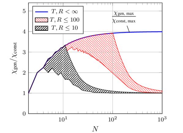
Figure 1: Ratio between the maximal value of $\chi_{\text{gen}}$ (for the case $Q=1$) and the maximal value of $\chi_{\text{const}}$ as a function of $N$, with and without a constraint on the maximal number of antennas. The shaded areas indicate the regions of $\chi_{\text{gen}}/\chi_{\text{const}}$ delimited by the upper bound (17) and lower bound (4) on $\chi_{\text{gen}}$.

Fig. 1 shows the ratio between the maximal value of $\chi_{\text{gen}}$ (for $Q=1$) and the maximal value of $\chi_{\text{const}}$ as a function of $N$. Because for the generic block-fading model the optimal number of receive antennas grows quadratically with $N$, which may yield an unreasonably large number of antennas for practically relevant values of $N$ (e.g., $1000$ symbols or more), in Fig. 1 we also show the ratio between the maximal values of $\chi_{\text{gen}}$ and $\chi_{\text{const}}$ under a constraint on the maximal number of antennas. For the case $R<T(N-1)/(N-T)$, which is relevant in the constrained setting, our upper and lower bounds on $\chi_{\text{gen}}$ (see (17) and (4) below) do not match. The degrees-of-freedom region delimited by the two bounds is represented in Fig. 1 by shaded areas. One can see from Fig. 1 that $\chi_{\text{gen, max}}$ is about four times $\chi_{\text{const, max}}$ when $N$ grows large. However, when the maximal number of transmit and receive antennas is constrained, the ratio $\chi_{\text{gen}}/\chi_{\text{const}}$ converges to $1$.

We emphasize that the only difference between the channel models (3) and (1) is that the generic (but deterministic) vectors $\bm{z}_{r,t}$ of (3) are replaced by the all-one vector in (1). It is important to note that the generic vectors $\bm{z}_{r,t}$ for which (5) holds include vectors that are arbitrarily close to the all-one vector. Hence, arbitrarily small perturbations of the constant block-fading model may result in a significant increase in the number of degrees of freedom. As we will demonstrate, the potential increase in the number of the degrees of freedom obtained when going from (1) to (3) is due to the fact that, under the generic block-fading model (3), the received signal vectors in the absence of noise span a subspace of higher dimension than under the constant block-fading model (1). We conclude that the commonly used constant block-fading model results in largely pessimistic capacity estimates at high SNR.

I-D Proof Techniques

To establish (5), we derive upper and lower bounds on capacity that match asymptotically (i.e., in terms of degrees of freedom). A similar approach was recently used in [11] to establish the degrees of freedom for the single-input multiple-output (SIMO) case. However, the proof techniques in [11] cannot be directly applied to the MIMO setting. A key step in [11] to obtain a tight lower bound on the number of degrees of freedom for the SIMO setting is to perform a change of variables using specific one-to-one mappings that relate the channel gains, the input signals, and the noiseless output signals. Unfortunately, the corresponding mappings for the MIMO case are not one-to-one, and hence the change-of-variable argument used in [11] cannot be applied. To overcome this problem, we invoke Bézout’s theorem in algebraic geometry [16, Prop. B.2.7] and show that these mappings are at least finite-to-one almost everywhere. We also derive a bound on the change of differential entropy that occurs when a random variable undergoes a finite-to-one mapping. Finally, we use a property of subharmonic functions [17, Th. 2.6.2.1] to establish that a term appearing in this change of differential entropy is finite.

I-E Notation

Sets are denoted by calligraphic letters (e.g., $\mathcal{I}$), and $|\mathcal{I}|$ denotes the cardinality of the set $\mathcal{I}$. The indicator function of a set $\mathcal{I}$ is denoted by $\mathbbmss{1}_{\mathcal{I}}$. Sets of sets are denoted by fraktur letters (e.g., $\mathfrak{M}$). The set of natural numbers (including zero) $\{0,1,2,\dots\}$ is denoted as $\mathbb{N}$. We use the notation $[M\!:\!N]$ to indicate the set $\{n\in\mathbb{N}:M\leq n\leq N\}$ for $M,N\!\in\!\mathbb{N}$. Boldface uppercase and lowercase letters denote matrices and vectors, respectively. Sans serif letters denote random quantities, e.g., $\bm{\mathsf{A}}$ is a random matrix, $\bm{\mathsf{x}}$ is a random vector, and $\mathsf{s}$ is a random scalar ($\bm{A},\bm{x}$, and $s$ denote the deterministic counterparts). The superscripts ${}^{\operatorname{T}}$ and ${}^{\operatorname{H}}$ stand for transposition and Hermitian transposition, respectively. The all-zero vector or matrix of appropriate size is written as $\bm{0}$, and the $M\times M$ identity matrix as $\mathbf{I}_{M}$. The entry in the $i$th row and $j$th column of a matrix $\bm{A}$ is denoted by $[\bm{A}]^{j}_{i}$, and the $i$th entry of a vector $\bm{x}$ by $[\bm{x}]_{i}$. For an $M\times N$ matrix $\bm{A}$, we denote by ${[\bm{A}]}_{\mathcal{I}}^{\mathcal{J}}$, where $\mathcal{I}\subseteq[1\!:\!M]$ and $\mathcal{J}\subseteq[1\!:\!N]$, the $|\mathcal{I}|\times|\mathcal{J}|$ submatrix of $\bm{A}$ containing the entries $[\bm{A}]^{j}_{i}$ with $i\!\in\!\mathcal{I}$ and $j\!\in\!\mathcal{J}$; furthermore, we let ${[\bm{A}]}_{\mathcal{I}}\!\triangleq{[\bm{A}]}_{\mathcal{I}}^{[1:N]}$ and ${[\bm{A}]}^{\mathcal{J}}\!\triangleq{[\bm{A}]}_{[1:M]}^{\mathcal{J}}$. We denote by ${[\bm{x}]}_{\mathcal{I}}\in\mathbb{C}^{|\mathcal{I}|}$ the subvector of $\bm{x}$ containing the entries $[\bm{x}]_{i}$ with $i\in\mathcal{I}$. The diagonal matrix with the entries of $\bm{x}$ in its main diagonal is denoted by $\operatorname{diag}(\bm{x})$. We let $\operatorname{diag}(\bm{A}_{1},\dots,\bm{A}_{K})$ be the block-diagonal matrix having the matrices $\bm{A}_{1},\dots,\bm{A}_{K}$ on the main block diagonal. By $\lvert\bm{A}\rvert$ we denote the modulus of the determinant of the square matrix $\bm{A}$. For $x\!\in\!\mathbb{R}$, we define $\lfloor x\rfloor\triangleq\max\{m\!\in\!\mathbb{Z}:m\!\leq\!x\}$ and $\lceil x\rceil\triangleq\min\{m\!\in\!\mathbb{Z}:m\!\geq\!x\}$. We write $\mathbb{E}[\cdot]$ for the expectation operator, and $\bm{\mathsf{x}}\sim\mathcal{CN}(\bm{0},\bm{\Sigma})$ to indicate that $\bm{\mathsf{x}}$ is a circularly symmetric complex Gaussian random vector with covariance matrix $\bm{\Sigma}$. The Jacobian matrix of a differentiable function $\phi$ is written as $\bm{J}_{\phi}$. For a function $\phi$ with domain $\mathcal{D}$ and a subset $\widetilde{\mathcal{D}}\subseteq\mathcal{D}$, we denote by $\phi\big{|}_{\widetilde{\mathcal{D}}}$ the restriction of $\phi$ to the domain $\widetilde{\mathcal{D}}$. We use the Landau notation $f(\rho)=\mathcal{O}(g(\rho))$ to indicate that there exist constants $c_{1},c_{2}>0$ such that $\lvert f(\rho)\rvert\leq c_{1}\,\lvert g(\rho)\rvert$ for $\rho>c_{2}$. Similarly, we use $f(\rho)=o(g(\rho))$ to indicate that for every $\varepsilon>0$ there exists a constant $c_{3}>0$ such that $\lvert f(\rho)\rvert\leq\varepsilon\,\lvert g(\rho)\rvert$ for $\rho>c_{3}$.

I-F Organization of the Paper

The rest of this paper is organized as follows. The system model is formulated in Section II. In Section III, we present and discuss our main result on the number of degrees of freedom of the generic block-fading MIMO channel. An underlying upper bound is stated and proved in Section IV, and a corresponding lower bound is given in Section V. In Section VI and in four appendices, we provide a proof of the lower bound.

II System Model

We consider a MIMO channel with $T$ transmit and $R$ receive antennas. The discrete-time fading process associated with each transmit-receive antenna pair conforms to a block-fading model, which results in the following channel input-output relations within a given block of $N$ channel uses:

$$\bm{\mathsf{y}}_{r}\hskip 0.85358pt=\,\sqrt{\frac{\rho}{T}}\!\sum_{t\in[1:T]}\!\operatorname{diag}(\bm{\mathsf{h}}_{r,t})\,\bm{\mathsf{x}}_{t}\hskip 0.85358pt+\,\bm{\mathsf{w}}_{r}\,,\quad r\in[1\!:\!R]\,.$$ (6)

Here, $\bm{\mathsf{x}}_{t}\in\mathbb{C}^{N}$ is the signal vector originating from the $t$th transmit antenna; $\bm{\mathsf{y}}_{r}\in\mathbb{C}^{N}$ is the signal vector at the $r$th receive antenna; $\bm{\mathsf{h}}_{r,t}\sim\mathcal{CN}(\bm{0},\bm{\Sigma}_{r,t})$ is the vector of $N$ channel coefficients between the $t$th transmit antenna and the $r$th receive antenna; $\bm{\mathsf{w}}_{r}\sim\mathcal{CN}(\bm{0},\mathbf{I}_{N})$ is the noise vector at the $r$th receive antenna; and $\rho\in\mathbb{R}^{+}$ is the SNR. The vectors $\bm{\mathsf{h}}_{r,t}$ and $\bm{\mathsf{w}}_{r}$ are assumed to be mutually independent and independent across $r\in[1\!:\!R]$ and $t\in[1\!:\!T]$, and to change in an independent fashion from block to block (“block-memoryless” assumption). The transmitted signal vectors $\bm{\mathsf{x}}_{t}$ are assumed to be independent of the vectors $\bm{\mathsf{h}}_{r,t}$ and $\bm{\mathsf{w}}_{r}$. We consider the noncoherent setting, where transmitter and receiver know the covariance matrix $\bm{\Sigma}_{r,t}$ of $\bm{\mathsf{h}}_{r,t}$ but have no a priori knowledge of the realization of $\bm{\mathsf{h}}_{r,t}$.

Because the covariance matrix $\bm{\Sigma}_{r,t}$ is positive-semidefinite, it can be factorized as

$$\bm{\Sigma}_{r,t}=\bm{Z}_{r,t}\bm{Z}_{r,t}^{\operatorname{H}}$$

with $\bm{Z}_{r,t}\in\mathbb{C}^{N\times Q}$ and $Q=\operatorname{rank}(\bm{\Sigma}_{r,t})=\operatorname{rank}(\bm{Z}_{r,t})$. We can then rewrite the channel coefficient vectors $\bm{\mathsf{h}}_{r,t}$ in terms of $\bm{Z}_{r,t}$ as in (4), i.e.,

$$\bm{\mathsf{h}}_{r,t}\hskip 0.85358pt=\hskip 0.85358pt\bm{Z}_{r,t}\bm{\mathsf{s}}_{r,t}$$ (7)

where $\bm{\mathsf{s}}_{r,t}\in\mathbb{C}^{Q}$, $\bm{\mathsf{s}}_{r,t}\sim\mathcal{CN}(\bm{0},\mathbf{I}_{Q})$. Using (7), the $R$ input-output relations (6) can be rewritten as

$$\bm{\mathsf{y}}_{r}\hskip 0.85358pt=\,\sqrt{\frac{\rho}{T}}\!\sum_{t\in[1:T]}\!\operatorname{diag}(\bm{Z}_{r,t}\bm{\mathsf{s}}_{r,t})\,\bm{\mathsf{x}}_{t}\hskip 0.85358pt+\,\bm{\mathsf{w}}_{r}\,,\quad r\in[1\!:\!R]\vspace*{-.5mm}$$ (8)

or in stacked form as

$$\bm{\mathsf{y}}\,=\hskip 0.85358pt\sqrt{\frac{\rho}{T}}\hskip 0.85358pt\bar{\bm{\mathsf{y}}}\hskip 0.85358pt+\hskip 0.85358pt\bm{\mathsf{w}},\quad\text{ with }\bar{\bm{\mathsf{y}}}\triangleq\bm{\mathsf{B}}\bm{\mathsf{s}}$$ (9)

where $\bm{\mathsf{y}}\!\triangleq(\bm{\mathsf{y}}_{1}^{\operatorname{T}}\cdots\bm{\mathsf{y}}_{R}^{\operatorname{T}})^{\operatorname{T}}\in\mathbb{C}^{RN}\!$, $\bm{\mathsf{w}}\!\triangleq(\bm{\mathsf{w}}_{1}^{\operatorname{T}}\cdots\bm{\mathsf{w}}_{R}^{\operatorname{T}})^{\operatorname{T}}\in\mathbb{C}^{RN}$, $\bm{\mathsf{s}}\triangleq(\bm{\mathsf{s}}_{1}^{\operatorname{T}}\cdots\bm{\mathsf{s}}_{R}^{\operatorname{T}})^{\operatorname{T}}\in\mathbb{C}^{RTQ}$ with $\bm{\mathsf{s}}_{r}\triangleq(\bm{\mathsf{s}}_{r,1}^{\operatorname{T}}\cdots$ $\bm{\mathsf{s}}_{r,T}^{\operatorname{T}})^{\operatorname{T}}\in\mathbb{C}^{TQ}$, and

$$\bm{\mathsf{B}}\triangleq\begin{pmatrix}\bm{\mathsf{B}}_{1}\\[-4.2679pt] &\ddots\\[-4.2679pt] &&\bm{\mathsf{B}}_{R}\end{pmatrix}\in\mathbb{C}^{RN\times RTQ},$$

$$\rule{22.76219pt}{0.0pt}\text{ with }\bm{\mathsf{B}}_{r}\triangleq(\bm{\mathsf{X}}_{1}\bm{Z}_{r,1}\cdots\bm{\mathsf{X}}_{T}\bm{Z}_{r,T})\in\mathbb{C}^{N\times TQ}$$ (10)

where $\bm{\mathsf{X}}_{t}\triangleq\operatorname{diag}(\bm{\mathsf{x}}_{t})\in\mathbb{C}^{N\times N}$. For later use, we also define $\bm{\mathsf{x}}\triangleq(\bm{\mathsf{x}}_{1}^{\operatorname{T}}\cdots\bm{\mathsf{x}}_{T}^{\operatorname{T}})^{\operatorname{T}}\in\mathbb{C}^{TN}$ and

$$\bm{Z}\hskip 0.85358pt\triangleq\hskip 0.85358pt\begin{pmatrix}\bm{Z}_{1,1}&\cdots&\bm{Z}_{1,T}\\[-1.42262pt] \vdots&&\vdots\\[-2.27621pt] \bm{Z}_{R,1}&\cdots&\bm{Z}_{R,T}\end{pmatrix}\in\mathbb{C}^{RN\times TQ}.$$

The matrix $\bm{Z}$ contains all information about the correlation of the channel coefficients $\bm{\mathsf{h}}_{r,t}$ (recall that $\bm{\Sigma}_{r,t}=\bm{Z}_{r,t}\bm{Z}_{r,t}^{\operatorname{H}}$). We will refer to $\bm{Z}$ as coloring matrix and use the phrase “for a generic coloring matrix $\bm{Z}$” to indicate that a property holds for almost every matrix $\bm{Z}$. Here, “almost every” is understood in the precise mathematical sense that the set of all matrices $\bm{Z}$ for which the property does not hold has Lebesgue measure zero.

In the special (nongeneric) case where $Q=1$ and each $\bm{Z}_{r,t}\in\mathbb{C}^{N\times 1}$ is the all-one vector, (8) reduces to the input-output relation of the constant block-fading model given by (cf. (1))

$$\bm{\mathsf{y}}_{r}\hskip 0.85358pt=\,\sqrt{\frac{\rho}{T}}\!\sum_{t\in[1:T]}\!\mathsf{s}_{r,t}\,\bm{\mathsf{x}}_{t}\hskip 0.85358pt+\,\bm{\mathsf{w}}_{r}\,,\quad r\in[1\!:\!R]\,.\vspace*{-.5mm}$$ (11)

III Characterization of the Number of Degrees of Freedom

III-A Main Result

Because of the block-memoryless assumption, the coding theorem in [18, Section 7.3] implies that the capacity of the channel (8) is given by

$$C(\rho)\hskip 0.85358pt=\hskip 0.85358pt\frac{1}{N}\sup I(\bm{\mathsf{x}}\hskip 0.85358pt;\bm{\mathsf{y}})\,.$$ (12)

Here, $I(\cdot\hskip 0.85358pt;\cdot)$ denotes mutual information [19, p. 251] and the supremum is taken over all probability distributions of $\bm{\mathsf{x}}$ that satisfy the average-power constraint

$$\mathbb{E}[\|\bm{\mathsf{x}}\|^{2}]\hskip 0.85358pt\leq\hskip 0.85358ptTN\,.$$ (13)

The number of degrees of freedom is defined as

$$\chi\hskip 0.85358pt\triangleq\lim_{\rho\to\infty}\frac{C(\rho)}{\log\rho}$$ (14)

which corresponds to the expansion

$$C(\rho)=\chi\log\rho+o(\log\rho)\,.$$ (15)

Our main result is stated in the following theorem.

Theorem 1:

Let $T\!<N/Q$ and $R\geq T(N-1)/(N-TQ)$. For a channel conforming to the generic block-fading model, i.e., the channel (8) with generic coloring matrix $\bm{Z}$, the number of degrees of freedom is given by

$$\chi_{\text{gen}}=\hskip 0.85358ptT\bigg{(}1-\frac{1}{N}\bigg{)}\,.$$ (16)

Proof:

In Section IV, we will show that $\chi_{\text{gen}}$ is upper-bounded by $T\hskip 0.85358pt(1-1/N)$ for all choices of $T,R,N,Q,$ and $\bm{Z}$. In Section V, we will show that this upper bound is achievable when $T\!<N/Q$, $R\geq T(N-1)/(N-TQ)$, and $\bm{Z}$ is generic (see Corollary 5). ∎

III-B Degrees of Freedom Gain

As discussed in Section I, (16) implies that the maximal achieveable number of degrees of freedom in the generic block-fading model can be about four times as large as the number of degrees of freedom in the constant block-fading model (2). We will now provide some intuition regarding this gain. For concreteness, we consider the case $T=2,R=3,Q=1,N=4$. In this case, (2) and (16) give $\chi_{\text{const}}=1$ and $\chi_{\text{gen}}=3/2$, respectively.

The number of degrees of freedom characterizes the channel capacity in a regime where the noise can “effectively” be ignored. Thus, according to the intuitive argumentation in [12, Section III], the number of degrees of freedom should be equal to the number of entries of $\bm{\mathsf{x}}\in\mathbb{C}^{8}$ that can be deduced from the corresponding received vector $\bm{\mathsf{y}}\in\mathbb{C}^{12}$ in the absence of noise, divided by the block length $N\!=4$.

In the constant block-fading model (11), the noiseless received vectors $\bar{\bm{\mathsf{y}}}_{r}=\mathsf{s}_{r,1}\bm{\mathsf{x}}_{1}+\mathsf{s}_{r,2}\hskip 0.85358pt\bm{\mathsf{x}}_{2}$, $r=1,2,3$ belong to the two-dimensional subspace spanned by $\{\bm{\mathsf{x}}_{1},\bm{\mathsf{x}}_{2}\}$. Hence, the received vectors $\bar{\bm{\mathsf{y}}}_{1},\bar{\bm{\mathsf{y}}}_{2},\bar{\bm{\mathsf{y}}}_{3}$ are linearly dependent, and two of them contain all the information available about $\bm{\mathsf{x}}$. From two of the received vectors, we obtain $2\cdot 4$ scalar equations in $8+4$ scalar variables ($\bm{\mathsf{x}},\mathsf{s}_{1,1},\mathsf{s}_{1,2},\mathsf{s}_{2,1},\mathsf{s}_{2,2}$). Since we do not have control of the variables $\mathsf{s}_{r,t}$, one way to reconstruct $\bm{\mathsf{x}}$ is to fix four of its entries (or, equivalently, to transmit four pilot symbols) to obtain eight equations in eight variables. By solving this system of equations, we obtain the remaining four entries of $\bm{\mathsf{x}}$. Hence, we can deduce four entries of $\bm{\mathsf{x}}$ from $\bar{\bm{\mathsf{y}}}$. We conclude that the number of degrees of freedom is $4/4=1$, which is in agreement with (2).

In the generic block-fading model (8), on the other hand, the received vectors without noise

$$\bar{\bm{\mathsf{y}}}_{r}=\operatorname{diag}(\bm{Z}_{r,1}\mathsf{s}_{r,1})\hskip 0.85358pt\bm{\mathsf{x}}_{1}+\operatorname{diag}(\bm{Z}_{r,2}\mathsf{s}_{r,2})\hskip 0.85358pt\bm{\mathsf{x}}_{2},\quad r=1,2,3$$

span a three-dimensional subspace almost surely. Hence, we obtain a system of $3\cdot 4$ equations in $8+6$ variables ($\bm{\mathsf{x}},\mathsf{s}_{1,1},\mathsf{s}_{1,2},\mathsf{s}_{2,1},\mathsf{s}_{2,2},\mathsf{s}_{3,1},\mathsf{s}_{3,2}$). Fixing two entries of $\bm{\mathsf{x}}$, we are able to recover the remaining six entries. Hence, the number of degrees of freedom is $6/4=3/2$, which is in agreement with (16).

This argument suggests that the reason why the generic block-fading model yields a larger number of degrees of freedom than the constant block-fading model is that the noiseless received vectors span a subspace of $\mathbb{C}^{N}$ of higher dimension.

IV Upper Bound

The following upper bound on the number of degrees of freedom of the channel (8) holds for every $T$, $R$, $Q$, $N$, and $\bm{Z}$. The assumption of a generic coloring matrix $\bm{Z}$ is not required.

Theorem 2:

The number of degrees of freedom of the channel (8) satisfies

$$\chi_{\text{gen}}\hskip 0.85358pt\leq\hskip 0.85358ptT\bigg{(}1-\frac{1}{N}\bigg{)}\,.$$ (17)

Proof:

We will show that the number of degrees of freedom is upper-bounded by $T$ times the number of degrees of freedom of a constant block-fading SIMO channel; the result then follows from (2). To this end, we will rewrite each output vector $\bm{\mathsf{y}}_{r}$ as the sum of the output vectors of $T$ SIMO systems with $RQ$ receive antennas each. This will be achieved by splitting the additive noise variables appropriately.

From (8), the $i$th entry of the received vector $\bm{\mathsf{y}}_{r}$ is given by

$$[\bm{\mathsf{y}}_{r}]_{i}=\hskip 0.85358pt\sqrt{\frac{\rho}{T}}\!\sum_{t\in[1:T]}\sum_{q\in[1:Q]}\!\![\bm{Z}_{r,t}]^{q}_{i}\hskip 0.85358pt[\bm{\mathsf{s}}_{r,t}]_{q}\hskip 0.85358pt[\bm{\mathsf{x}}_{t}]_{i}\hskip 0.85358pt+\hskip 0.85358pt[\bm{\mathsf{w}}_{r}]_{i}$$ (18)

for $r\in[1\!:\!R]$. We first decompose the noise variables according to

$$[\bm{\mathsf{w}}_{r}]_{i}=\sum_{t\in[1:T]}\sum_{q\in[1:Q]}\frac{[\bm{Z}_{r,t}]^{q}_{i}\hskip 0.85358pt}{\sqrt{KT}}[\tilde{\bm{\mathsf{w}}}_{q,r,t}]_{i}+[\bm{\mathsf{w}}^{\prime}_{r}]_{i}\,.$$ (19)

Here, all $[\tilde{\bm{\mathsf{w}}}_{q,r,t}]_{i}$ and $[\bm{\mathsf{w}}^{\prime}_{r}]_{i}$ are mutually independent and independent of all $\bm{\mathsf{x}}_{t}$ and $\bm{\mathsf{s}}_{r,t}$. Furthermore, $[\tilde{\bm{\mathsf{w}}}_{q,r,t}]_{i}\sim\mathcal{CN}(0,1)$,

$$[\bm{\mathsf{w}}^{\prime}_{r}]_{i} \sim\mathcal{CN}\bigg{(}0,1-\sum_{t\in[1:T]}\sum_{q\in[1:Q]}\frac{\lvert[\bm{Z}_{r,t}]^{q}_{i}\rvert^{2}}{KT}\bigg{)}\,,$$

and $K$ is a finite constant satisfying

$$K>\max_{r\in[1:R],\hskip 0.85358pti\in[1:N]}\sum_{t\in[1:T]}\sum_{q\in[1:Q]}\lvert[\bm{Z}_{r,t}]^{q}_{i}\rvert^{2}\,.$$

We next define $T$ “virtual” constant block-fading SIMO channels with $RQ$ receive antennas each:

$$[\tilde{\bm{\mathsf{y}}}_{q,r,t}]_{i}=\hskip 0.85358pt\sqrt{K\rho}\,\hskip 0.85358pt[\bm{\mathsf{s}}_{r,t}]_{q}\hskip 0.85358pt[\bm{\mathsf{x}}_{t}]_{i}+\hskip 0.85358pt[\tilde{\bm{\mathsf{w}}}_{q,r,t}]_{i}\,,$$

$$\rule{71.13188pt}{0.0pt}i\!\in\![1\!:\!N],r\!\in\![1\!:\!R],q\in[1\!:\!Q]$$ (20)

for $t\!\in\![1\!:\!T]$. Inserting (19) into (18) and using (IV), it can be verified that (18) can be rewritten as

$$[\bm{\mathsf{y}}_{r}]_{i}=\hskip 0.85358pt\frac{1}{\sqrt{KT}}\!\sum_{t\in[1:T]}\sum_{q\in[1:Q]}\![\bm{Z}_{r,t}]^{q}_{i}\hskip 0.85358pt[\tilde{\bm{\mathsf{y}}}_{q,r,t}]_{i}+\hskip 0.85358pt[\bm{\mathsf{w}}^{\prime}_{r}]_{i}\,.$$ (21)

Let $\tilde{\bm{\mathsf{y}}}_{t}\triangleq(\tilde{\bm{\mathsf{y}}}_{1,1,t}^{\operatorname{T}}\cdots\hskip 0.85358pt\tilde{\bm{\mathsf{y}}}_{Q,R,t}^{\operatorname{T}})^{\operatorname{T}}\!\in\mathbb{C}^{QRN}$. By (21), the random variable $\bm{\mathsf{y}}$ depends on $\bm{\mathsf{x}}$ only via the random variables $\{\tilde{\bm{\mathsf{y}}}_{t}\}_{t\in[1:T]}$. Hence, the data-processing inequality [18, eq. (2.3.19)] yields

$$I(\bm{\mathsf{x}}\hskip 0.85358pt;\bm{\mathsf{y}})\hskip 0.85358pt\leq\hskip 0.85358ptI(\bm{\mathsf{x}}\hskip 0.85358pt;\tilde{\bm{\mathsf{y}}}_{1},\dots,\tilde{\bm{\mathsf{y}}}_{T})\,.$$ (22)

The right-hand side of (22) can be upper-bounded as follows:

$$I(\bm{\mathsf{x}}\hskip 0.85358pt;\tilde{\bm{\mathsf{y}}}_{1},\dots,\tilde{\bm{\mathsf{y}}}_{T}) =h(\tilde{\bm{\mathsf{y}}}_{1},\dots,\tilde{\bm{\mathsf{y}}}_{T})\hskip 0.85358pt-\hskip 0.85358pth(\tilde{\bm{\mathsf{y}}}_{1},\dots,\tilde{\bm{\mathsf{y}}}_{T}|\hskip 0.85358pt\bm{\mathsf{x}})$$

$$\stackrel{{\scriptstyle(a)}}{{=}}h(\tilde{\bm{\mathsf{y}}}_{1},\dots,\tilde{\bm{\mathsf{y}}}_{T})\hskip 0.85358pt-\!\sum_{t\in[1:T]}\!h(\tilde{\bm{\mathsf{y}}}_{t}|\hskip 0.85358pt\bm{\mathsf{x}}_{t})$$

$$\stackrel{{\scriptstyle(b)}}{{\leq}}\!\sum_{t\in[1:T]}\!\!\big{[}h(\tilde{\bm{\mathsf{y}}}_{t})-h(\tilde{\bm{\mathsf{y}}}_{t}|\hskip 0.85358pt\bm{\mathsf{x}}_{t})\big{]}$$

$$=\sum_{t\in[1:T]}\!\!I(\bm{\mathsf{x}}_{t}\hskip 0.85358pt;\tilde{\bm{\mathsf{y}}}_{t})\,.$$ (23)

Here, $h(\cdot)$ denotes differential entropy [19, Ch. 8], $(a)$ holds because $\tilde{\bm{\mathsf{y}}}_{1},\dots,\tilde{\bm{\mathsf{y}}}_{T}$ are conditionally independent given $\bm{\mathsf{x}}$, and $(b)$ follows from the chain rule for differential entropy [19, Th. 8.6.2] and because conditioning does not increase differential entropy. Since (by assumption) the input vector $\bm{\mathsf{x}}$ satisfies the power constraint (13), we conclude that, trivially, also each subvector $\bm{\mathsf{x}}_{t}$ satisfies the individual power constraint $\mathbb{E}[\lVert\bm{\mathsf{x}}_{t}\rVert^{2}]\leq TN$. Thus, the SNR (i.e., the expected power of the noiseless received signal divided by the noise power) of each “virtual” constant block-fading SIMO channel (IV) is given by

$$\frac{\mathbb{E}[\lVert\sqrt{K\rho}\,[\bm{\mathsf{s}}_{r,t}]_{q}\bm{\mathsf{x}}_{t}\rVert^{2}]}{\mathbb{E}[\lVert\tilde{\bm{\mathsf{w}}}_{q,r,t}\rVert^{2}]} =\frac{K\rho\,\mathbb{E}[\lvert[\bm{\mathsf{s}}_{r,t}]_{q}\rvert^{2}]\,\mathbb{E}[\lVert\bm{\mathsf{x}}_{t}\rVert^{2}]}{\mathbb{E}[\lVert\tilde{\bm{\mathsf{w}}}_{q,r,t}\rVert^{2}]}$$

$$\leq\frac{K\rho\,TN}{N}$$

$$=TK\rho\,.$$

By (2) and (15), the capacity of a constant block-fading SIMO channel of SNR $TK\rho$ is of the form $(1-1/N)\log(TK\rho)+o(\log\rho)$. Since, by (12), the capacity is the supremum of the mutual information divided by the block length, we can upper-bound each mutual information $I(\bm{\mathsf{x}}_{t}\hskip 0.85358pt;\tilde{\bm{\mathsf{y}}}_{t})$, $t\in[1\!:\!T]$ by $N$ times the capacity. This results in

$$I(\bm{\mathsf{x}}_{t}\hskip 0.85358pt;\tilde{\bm{\mathsf{y}}}_{t}) \leq N\bigg{(}\Big{(}1-\frac{1}{N}\Big{)}\log(TK\rho)+o(\log\rho)\bigg{)}$$

$$=(N-1)\log(TK\rho)+o(\log\rho)\,.$$

Hence, continuing (22) and (23), we obtain

$$I(\bm{\mathsf{x}}\hskip 0.85358pt;\bm{\mathsf{y}}) \leq\sum_{t\in[1:T]}\!\!I(\bm{\mathsf{x}}_{t}\hskip 0.85358pt;\tilde{\bm{\mathsf{y}}}_{t})$$

$$\leq\,T(N-1)\log(TK\rho)\hskip 0.85358pt+\hskip 0.85358pto(\log\rho)$$

$$\stackrel{{\scriptstyle(a)}}{{=}}\,T(N-1)\log\rho\hskip 0.85358pt+\hskip 0.85358pto(\log\rho)$$ (24)

where $(a)$ holds because $\log(TK\rho)=\log\rho+\log(TK)$. Thus, the mutual information $I(\bm{\mathsf{x}};\bm{\mathsf{y}})$ with $\bm{\mathsf{x}}$ satisfying the power constraint (13) is upper-bounded by (IV). Inserting (IV) into (12) yields

$$C(\rho) \leq T\hskip 0.85358pt\frac{N\!-\!1}{N}\log\rho\hskip 0.85358pt+\hskip 0.85358pto(\log\rho)$$

from which (17) follows via (14). ∎

V Lower Bound

We first derive a lower bound on $\chi_{\text{gen}}$ assuming that $\widetilde{T}\leq\min\{T,R\}$ transmit antennas are effectively used (i.e., $\bm{\mathsf{x}}_{\widetilde{T}+1},\dots,\bm{\mathsf{x}}_{T}$ are set to zero). Then we maximize the lower bound by identifying the optimal number $\widetilde{T}$ of transmit antennas to use.

Proposition 3:

The number of degrees of freedom of the channel (8) for a generic coloring matrix $\bm{Z}$ is lower-bounded by

$$\chi_{\text{gen}}\,\geq\,\chi_{\text{low}}(\widetilde{T})\,\triangleq\,\min\bigg{\{}\widetilde{T}\bigg{(}1-\frac{1}{N}\bigg{)},R\bigg{(}1-\frac{\widetilde{T}Q}{N}\bigg{)}\bigg{\}}$$ (25)

for all $\widetilde{T}\leq\min\{T,R\}$.

Proof:

See Section VI.∎

The minimum in (25) is given by $\chi_{\text{low}}(\widetilde{T})=\widetilde{T}(1-1/N)$ when the number $R$ of receive antennas is large enough (i.e., $R\geq\widetilde{T}(N-1)/(N-\widetilde{T}Q)$). In contrast, $\chi_{\text{low}}(\widetilde{T})=R(1-\widetilde{T}Q/N)$ when the number of degrees of freedom is constrained by the limited number of receive antennas (i.e., $R<\widetilde{T}(N-1)/(N-\widetilde{T}Q)$).

The main result of this section is stated in the following theorem.

Theorem 4:

The number of degrees of freedom of the channel (8) for a generic coloring matrix $\bm{Z}$ is lower-bounded by

$$\chi_{\text{gen}}\geq\chi^{*}_{\text{low}} \triangleq\max_{\widetilde{T}\leq\min\{T,R\}}\chi_{\text{low}}(\widetilde{T})$$

$$=\begin{cases}T\bigg{(}1-\dfrac{1}{N}\bigg{)},&\text{ if }T\leq T_{\text{opt}}\\ \eta,&\text{ if }T>T_{\text{opt}}\end{cases}$$ (26)

where

$$T_{\text{opt}}\,\triangleq\,\frac{RN}{N+RQ-1}$$ (27)

and

$$\eta\,\triangleq\,\max\bigg{\{}R\bigg{(}1-\frac{\lceil T_{\text{opt}}\rceil Q}{N}\bigg{)},\lfloor T_{\text{opt}}\rfloor\bigg{(}1-\frac{1}{N}\bigg{)}\bigg{\}}\,.$$ (28)

Proof:

The idea behind the bound $\chi^{*}_{\text{low}}$ in (4) is to obtain the tightest (i.e., largest) of the lower bounds $\chi_{\text{low}}(\widetilde{T})$ in (25) for $T$ transmit antennas by maximizing $\chi_{\text{low}}(\widetilde{T})$ with respect to the number of effectively used transmit antennas $\widetilde{T}\leq\min\{T,R\}$. According to (25), $\chi_{\text{low}}(\widetilde{T})$ is the minimum of two quantities where the first, $\widetilde{T}(1-1/N)$, is monotonically increasing in $\widetilde{T}$ and the second, $R(1-\widetilde{T}Q/N)$, is monotonically decreasing in $\widetilde{T}$. Hence, $\chi_{\text{low}}(\widetilde{T})$ attains its maximum at the intersection point $T_{\text{opt}}$ defined in (27). If $T\leq T_{\text{opt}}$, we are for all $\widetilde{T}\leq\min\{T,R\}$ in the regime where $\chi_{\text{low}}(\widetilde{T})$ is monotonically increasing, and thus the best choice is to use $\widetilde{T}=T$ transmit antennas (note that because $T\leq T_{\text{opt}}\stackrel{{\scriptstyle\eqref{eq:topt}}}{{\leq}}RN/N=R$, the choice $\widetilde{T}=T$ in Proposition 3 is possible). Thus, in this case we have $\chi^{*}_{\text{low}}=\chi_{\text{low}}(T)=T(1-1/N)$, which yields the first case in (4). If $T>T_{\text{opt}}$, we would like to use $T_{\text{opt}}$ transmit antennas, but we have to take into account that $T_{\text{opt}}$ may be noninteger. Thus, we take the maximum of the bounds $\chi_{\text{low}}(\widetilde{T})$ resulting from the closest integers, $\chi_{\text{low}}(\lfloor T_{\text{opt}}\rfloor)$ and $\chi_{\text{low}}(\lceil T_{\text{opt}}\rceil)$, which yields $\eta$ in (28). This concludes the proof.∎

Remark 1:

For $N\geq 2$, the optimal number of transmit antennas $T_{\text{opt}}$ is upper-bounded as follows:

$$T_{\text{opt}}<\frac{N}{Q}\,.$$ (29)

In fact, $T_{\text{opt}}=RN/(N+RQ-1)<RN/(RQ)=N/Q$.

Remark 2:

For $N=Q\geq 2$, we have by (29) that $T_{\text{opt}}<1$. Hence, $T>T_{\text{opt}}$ and thus, by (4) and (28), $\chi^{*}_{\text{low}}=\eta=\max\big{\{}R(1-Q/N),0\big{\}}=0$. Similarly, we obtain for $N=1$ that $\chi_{\text{low}}(\widetilde{T})\leq 0$ for all $\widetilde{T}$, which yields $\chi^{*}_{\text{low}}\leq 0$. Hence, our lower bound $\chi^{*}_{\text{low}}$ is trivial. In these scenarios, the capacity grows double-logarithmically in the SNR $\rho$ [20, 21].

Remark 3:

The lower bound $\chi^{*}_{\text{low}}$ in (4) can be equivalently expressed as

$$\chi^{*}_{\text{low}}\hskip 0.85358pt=\,\min\bigg{\{}T\bigg{(}1-\frac{1}{N}\bigg{)},\eta\bigg{\}}\,.\vspace{1.5mm}$$

Corollary 5:

Let $N\geq 2$. For the lower bound $\chi_{\text{low}}^{*}$ in Theorem 4, the following properties hold:

1. For $T\geq N/Q$, we have $T>T_{\text{opt}}$ and $\chi_{\text{low}}^{*}=\eta$.

2. For $T<N/Q$ and $R\geq T(N-1)/(N-TQ)$, we have $T\leq T_{\text{opt}}$ and $\chi_{\text{low}}^{*}=T(1-1/N)$.

3. For $T<N/Q$ and $R<T(N-1)/(N-TQ)$, we have $T>T_{\text{opt}}$ and $\chi_{\text{low}}^{*}=\eta$.

4. For fixed $N$ and $Q$, $\chi_{\text{low}}^{*}$ attains its maximal value for $T=\lfloor(N-1)/Q\rfloor$ transmit antennas and $R=\lceil(N-1)^{2}/Q\rceil$ receive antennas; this maximal value of $\chi^{*}_{\text{low}}$ equals $\lfloor(N-1)/Q\rfloor(1-1/N)$.

Proof:

By (29), the inequality $T\geq N/Q$ implies $T>T_{\text{opt}}$, from which Property (i) follows by (4). For $T<N/Q$, the following equivalence holds:

$$T\leq T_{\text{opt}}\stackrel{{\scriptstyle\eqref{eq:topt}}}{{=}}\frac{RN}{N+RQ-1}\quad \Leftrightarrow\quad T\frac{N-1}{N-TQ}\leq R\,.$$

Thus, the conditions in Properties (ii) and (iii) imply $T\leq T_{\text{opt}}$ and $T>T_{\text{opt}}$, respectively, and the expressions of $\chi_{\text{low}}^{*}$ given in Properties (ii) and (iii) follow immediately from the case distinction in (4).

To prove Property (iv), we first show that $\chi_{\text{low}}^{*}\leq\lfloor(N-1)/Q\rfloor(1-1/N)$ for arbitrary $T$ and $R$. Subsequently, we will show that this upper bound is achievable for the proposed number of antennas. We first note that for each $\widetilde{T}\leq N/Q$, the lower bound $\chi_{\text{low}}(\widetilde{T})$ in (25) is monotonically nondecreasing in $R$. Furthermore, for $\widetilde{T}>N/Q$, $\chi_{\text{low}}(\widetilde{T})$ is negative and can be ignored in the maximization process, i.e., we have $\chi_{\text{low}}^{*}=\max_{\widetilde{T}\leq\min\{T,R,N/Q\}}\chi_{\text{low}}(\widetilde{T})$. This implies that $\chi_{\text{low}}^{*}$ is—as a maximum of nondecreasing functions—also monotonically nondecreasing in $R$. Hence, to obtain an upper bound on $\chi_{\text{low}}^{*}$, we can assume $R$ arbitrarily large without loss of generality. We choose $R>(N-1)^{2}/Q$. Simple algebraic manipulations yield the equivalence

$$R>\frac{(N-1)^{2}}{Q}\quad \Leftrightarrow\quad T_{\text{opt}}=\frac{RN}{N+RQ-1}>\frac{N-1}{Q}\,.$$ (30)

This implies $\lceil T_{\text{opt}}\rceil Q>N-1$ and further, because both sides of this strict inequality are integers, that $\lceil T_{\text{opt}}\rceil Q\geq N$. Thus, the first argument of the maximum defining $\eta$ in (28) satisfies

$$R\bigg{(}1-\frac{\lceil T_{\text{opt}}\rceil Q}{N}\bigg{)}\leq R(1-1)=0$$

and, hence, $\eta$ reduces to $\eta=\lfloor T_{\text{opt}}\rfloor(1-1/N)$. By (4), we have that $\chi_{\text{low}}^{*}$ is either equal to $T(1-1/N)$ (for $T\leq T_{\text{opt}}$) or equal to $\eta=\lfloor T_{\text{opt}}\rfloor(1-1/N)$ (for $T>T_{\text{opt}}$). In both cases we have $\chi_{\text{low}}^{*}\leq\lfloor T_{\text{opt}}\rfloor(1-1/N)$. Since $\lfloor T_{\text{opt}}\rfloor\leq\lfloor(N-1)/Q\rfloor$ by (29), this implies $\chi_{\text{low}}^{*}\leq\lfloor(N-1)/Q\rfloor(1-1/N)$.

It remains to be shown that this upper bound is achievable. For $R=\lceil(N-1)^{2}/Q\rceil\geq(N-1)^{2}/Q$, we obtain (see (30) with “$>$” replaced by “$\geq$”) that $T_{\text{opt}}\geq(N-1)/Q$. Hence, for $T=\lfloor(N-1)/Q\rfloor\leq T_{\text{opt}}$, the lower bound (4) simplifies to $\chi_{\text{low}}^{*}=T(1-1/N)=\lfloor(N-1)/Q\rfloor(1-1/N)$. Thus, we have shown that $\chi_{\text{low}}^{*}$ is maximized for $T=\lfloor(N-1)/Q\rfloor$ and $R=\lceil(N-1)^{2}/Q\rceil$ and its maximum equals $\lfloor(N-1)/Q\rfloor(1-1/N)$. ∎

Remark 4:

Property (ii) in Corollary 5 shows that for a fixed $T\!<N/Q$, we can achieve $\chi^{*}_{\text{low}}\!=T(1-1/N)$ by using a sufficiently large number of receive antennas $R$. This coincides with the upper bound presented in Section IV. Thus, in this regime, the number of degrees of freedom grows linearly in the number of transmit antennas.

VI Proof of Proposition 3

In this section, we establish the lower bound (25). For $N\leq\widetilde{T}Q$, the inequality in (25) is trivially true, because in this case $R(1-\widetilde{T}Q/N)\leq 0$ and hence $\chi_{\text{low}}\leq 0$. Therefore, we focus on the case

$$N>\widetilde{T}Q$$

which will thus be assumed in the remainder of this section. Furthermore, recall that we assumed in Proposition 3 that $\widetilde{T}\leq\min\{T,R\}$. Thus, setting $\bm{\mathsf{x}}_{\widetilde{T}+1},\dots,\bm{\mathsf{x}}_{T}$ to zero, we can replace $T$ by $\widetilde{T}$ in the input-output relation (9) and the power constraint (13). Finally, we shall assume that

$$R\leq\bigg{\lceil}\frac{\widetilde{T}(N-1)}{N-\widetilde{T}Q}\bigg{\rceil}\,.$$

If more receive antennas are available, we simply turn them off. The following dimension counting argument provides some intuition on why the use of more than $\lceil\widetilde{T}(N-1)/(N-\widetilde{T}Q)\rceil$ receive antennas is not beneficial.

VI-A Dimension Counting

The noiseless received vector $\bar{\bm{\mathsf{y}}}=\bm{\mathsf{B}}\bm{\mathsf{s}}\in\mathbb{C}^{RN}$ in (9) corresponds to $RN$ polynomial equations. The unknown variables of these equations are the entries of the vectors $\bm{\mathsf{s}}_{r,t}\in\mathbb{C}^{Q}$, $r\in[1\!:\!R]$, $t\in[1\!:\!\widetilde{T}]$ ($R\widetilde{T}Q$ unknown variables) and of the transmitted signal vectors $\bm{\mathsf{x}}_{t}\in\mathbb{C}^{N}$, $t\in[1\!:\!\widetilde{T}]$ ($\widetilde{T}N$ unknown variables). Consider now a pair $(\bm{\mathsf{x}}_{t},\bm{\mathsf{s}}_{r,t})$, consisting of a transmitted signal vector $\bm{\mathsf{x}}_{t}$ and a fading vector $\bm{\mathsf{s}}_{r,t}$ that is a solution of $\bar{\bm{\mathsf{y}}}=\bm{\mathsf{B}}\bm{\mathsf{s}}$. Then the pair $(c_{t}\bm{\mathsf{x}}_{t},\bm{\mathsf{s}}_{r,t}/c_{t})$, where $c_{t}$ is an arbitrary nonzero constant, is also a solution of $\bar{\bm{\mathsf{y}}}=\bm{\mathsf{B}}\bm{\mathsf{s}}$. This implies that each $\bm{\mathsf{x}}_{t}$ can be recovered from $\bar{\bm{\mathsf{y}}}$ only up to a scaling factor. To resolve this ambiguity, we fix one entry in each $\bm{\mathsf{x}}_{t}$. Hence, the total number of unknown variables becomes $R\widetilde{T}Q+\widetilde{T}N-\widetilde{T}$. As long as the number of equations is larger than or equal to the number of unknown variables, i.e., $RN\geq R\widetilde{T}Q+\widetilde{T}N-\widetilde{T}$, we are able to recover the $N-1$ unknown entries of each $\bm{\mathsf{x}}_{t}$. The above condition is equivalent to $R\geq\widetilde{T}(N-1)/(N-\widetilde{T}Q)$. Hence, it is reasonable to consider only the case $R\leq\lceil\widetilde{T}(N-1)/(N-\widetilde{T}Q)\rceil$, as the received vectors resulting from the use of additional receive antennas would not help us gain more information about the transmit vectors $\{\bm{\mathsf{x}}_{t}\}_{t\in[1:\widetilde{T}]}$.

VI-B Bounding $I(\bm{\mathsf{x}}\hskip 0.85358pt;\bm{\mathsf{y}})$

By (12), the capacity $C(\rho)$ and, hence, $\chi_{\text{gen}}$ (cf. (14)) can be lower-bounded by evaluating $I(\bm{\mathsf{x}}\hskip 0.85358pt;\bm{\mathsf{y}})$ for any specific input distribution that satisfies the power constraint (13). In particular, in what follows, we will assume $\bm{\mathsf{x}}\sim\mathcal{CN}(\bm{0},\mathbf{I}_{\widetilde{T}N})$. Thus,

$$C(\rho)\geq\frac{1}{N}\,I(\bm{\mathsf{x}}\hskip 0.85358pt;\bm{\mathsf{y}})\,.$$ (31)

As

$$I(\bm{\mathsf{x}}\hskip 0.85358pt;\bm{\mathsf{y}})=h(\bm{\mathsf{y}})-h(\bm{\mathsf{y}}\hskip 0.85358pt|\hskip 0.85358pt\bm{\mathsf{x}})$$ (32)

we can lower-bound $I(\bm{\mathsf{x}}\hskip 0.85358pt;\bm{\mathsf{y}})$ by upper-bounding $h(\bm{\mathsf{y}}\hskip 0.85358pt|\hskip 0.85358pt\bm{\mathsf{x}})$ and lower-bounding $h(\bm{\mathsf{y}})$.

VI-B1 Upper Bound on $h(\bm{\mathsf{y}}|\bm{\mathsf{x}})$

It follows from (9) and (II) together with $\bm{\mathsf{s}}_{r,t}\sim\mathcal{CN}(\bm{0},\mathbf{I}_{Q})$ and $\bm{\mathsf{w}}_{r}\sim\mathcal{CN}(\bm{0},\mathbf{I}_{N})$ that $\bm{\mathsf{y}}$ is conditionally Gaussian given $\bm{\mathsf{x}}$, with conditional covariance matrix $(\rho/\widetilde{T})\hskip 0.85358pt\bm{\mathsf{B}}\bm{\mathsf{B}}^{\operatorname{H}}+\mathbf{I}_{RN}$ (note that $\bm{\mathsf{B}}=\bm{\mathsf{B}}(\bm{\mathsf{x}})$). Hence,

$$h(\bm{\mathsf{y}}\hskip 0.85358pt|\hskip 0.85358pt\bm{\mathsf{x}})=\mathbb{E}_{\bm{\mathsf{x}}}\bigg{[}\log\bigg{(}(\pi e)^{RN}\,\bigg{\lvert}\frac{\rho}{\widetilde{T}}\hskip 0.85358pt\bm{\mathsf{B}}\bm{\mathsf{B}}^{\operatorname{H}}+\mathbf{I}_{RN}\bigg{\rvert}\hskip 0.85358pt\bigg{)}\bigg{]}$$

according to [22, Th. 2]. By [23, Th. 1.3.20], $\big{\lvert}(\rho/\widetilde{T})\hskip 0.85358pt\bm{\mathsf{B}}\bm{\mathsf{B}}^{\operatorname{H}}+\mathbf{I}_{RN}\big{\rvert}=\big{\lvert}(\rho/\widetilde{T})\hskip 0.85358pt\bm{\mathsf{B}}^{\operatorname{H}}\bm{\mathsf{B}}+\mathbf{I}_{R\widetilde{T}Q}\big{\rvert}$. Furthermore, assuming without loss of generality that $\rho>\!1$ (note that we are only interested in the asymptotic regime $\rho\rightarrow\infty$), we have $\big{\lvert}(\rho/\widetilde{T})\hskip 0.85358pt\bm{\mathsf{B}}^{\operatorname{H}}\bm{\mathsf{B}}+\mathbf{I}_{R\widetilde{T}Q}\big{\rvert}\leq\big{\lvert}\rho\big{(}(1/\widetilde{T})\hskip 0.85358pt\bm{\mathsf{B}}^{\operatorname{H}}\bm{\mathsf{B}}+\mathbf{I}_{R\widetilde{T}Q}\big{)}\big{\rvert}=\rho^{R\widetilde{T}Q}\big{\lvert}(1/\widetilde{T})\hskip 0.85358pt\bm{\mathsf{B}}^{\operatorname{H}}\bm{\mathsf{B}}+\mathbf{I}_{R\widetilde{T}Q}\big{\rvert}$. Thus,

$$h(\bm{\mathsf{y}}\hskip 0.85358pt|\hskip 0.85358pt\bm{\mathsf{x}}) \leq\mathbb{E}_{\bm{\mathsf{x}}}\bigg{[}\log\bigg{(}(\pi e)^{RN}\rho^{R\widetilde{T}Q}\,\bigg{\lvert}\frac{1}{\widetilde{T}}\hskip 0.85358pt\bm{\mathsf{B}}^{\operatorname{H}}\bm{\mathsf{B}}+\mathbf{I}_{{R\widetilde{T}Q}}\bigg{\rvert}\hskip 0.85358pt\bigg{)}\bigg{]}$$

$$=R\widetilde{T}Q\log\rho+\mathbb{E}_{\bm{\mathsf{x}}}\bigg{[}\log\bigg{\lvert}\frac{1}{\widetilde{T}}\bm{\mathsf{B}}^{\operatorname{H}}\bm{\mathsf{B}}+\mathbf{I}_{{R\widetilde{T}Q}}\bigg{\rvert}\bigg{]}+\mathcal{O}(1).$$ (33)

By using Jensen’s inequality for the concave function $\log(\cdot)$, we obtain

$$\mathbb{E}_{\bm{\mathsf{x}}}\bigg{[}\log\hskip 0.85358pt\bigg{\lvert}\frac{1}{\widetilde{T}}\hskip 0.85358pt\bm{\mathsf{B}}^{\operatorname{H}}\bm{\mathsf{B}}\hskip 0.85358pt+\mathbf{I}_{{R\widetilde{T}Q}}\bigg{\rvert}\bigg{]}\leq\log\mathbb{E}_{\bm{\mathsf{x}}}\bigg{[}\bigg{\lvert}\frac{1}{\widetilde{T}}\hskip 0.85358pt\bm{\mathsf{B}}^{\operatorname{H}}\bm{\mathsf{B}}+\,\mathbf{I}_{{R\widetilde{T}Q}}\bigg{\rvert}\bigg{]}\,.$$ (34)

The right-hand side in (34) is independent of $\rho$ and the determinant $\big{\lvert}(1/\widetilde{T})\hskip 0.85358pt\bm{\mathsf{B}}^{\operatorname{H}}\bm{\mathsf{B}}+\,\mathbf{I}_{{R\widetilde{T}Q}}\big{\rvert}$ is some polynomial in the entries of $\bm{\mathsf{x}}$ and $\bm{\mathsf{x}}^{\operatorname{H}}$ (cf. (II)). Since $\bm{\mathsf{x}}\sim\mathcal{CN}(\bm{0},\mathbf{I}_{\widetilde{T}N})$, all moments of $\bm{\mathsf{x}}$, and, hence, the expectation $\mathbb{E}_{\bm{\mathsf{x}}}\big{[}\big{\lvert}(1/\widetilde{T})\hskip 0.85358pt\bm{\mathsf{B}}^{\operatorname{H}}\bm{\mathsf{B}}+\,\mathbf{I}_{{R\widetilde{T}Q}}\big{\rvert}\big{]}$, are finite. Therefore, the right-hand side in (34) is a finite constant with respect to $\rho$. Hence, (33) together with (34) implies

$$h(\bm{\mathsf{y}}\hskip 0.85358pt|\hskip 0.85358pt\bm{\mathsf{x}})\hskip 0.85358pt\leq\hskip 0.85358ptR\widetilde{T}Q\log\rho+\hskip 0.85358pt\mathcal{O}(1)\,.$$ (35)

VI-B2 Lower Bound on $h(\bm{\mathsf{y}})$

The dimension counting argument provided in Section VI-A suggests that $R\leq\lceil\widetilde{T}(N-1)/(N-\widetilde{T}Q)\rceil$ receive antennas are sufficient to identify all unknown input parameters. By comparing more carefully the number of equations $RN$ and the number of variables $R\widetilde{T}Q+\widetilde{T}N-\widetilde{T}$, we see that we can get rid of

$$\ell\triangleq\max\{0,RN-(R\widetilde{T}Q+\widetilde{T}N-\widetilde{T})\}$$ (36)

equations. Since we assumed that $R\leq\lceil\widetilde{T}(N-1)/(N-\widetilde{T}Q)\rceil$ and $N>\widetilde{T}Q$, we have that

$$\ell =\max\{0,R(N-\widetilde{T}Q)-\widetilde{T}(N-1)\}$$

$$\leq\max\bigg{\{}0,\bigg{\lceil}\frac{\widetilde{T}(N-1)}{N-\widetilde{T}Q}\bigg{\rceil}(N-\widetilde{T}Q)-\widetilde{T}(N-1)\bigg{\}}$$

$$=\max\bigg{\{}0,\underbrace{\bigg{(}\bigg{\lceil}\frac{\widetilde{T}(N-1)}{N-\widetilde{T}Q}\bigg{\rceil}-\frac{\widetilde{T}(N-1)}{N-\widetilde{T}Q}\bigg{)}}_{\geq 0}\underbrace{(N-\widetilde{T}Q)}_{>0}\!\bigg{\}}$$

$$=\underbrace{\bigg{(}\bigg{\lceil}\frac{\widetilde{T}(N-1)}{N-\widetilde{T}Q}\bigg{\rceil}-\frac{\widetilde{T}(N-1)}{N-\widetilde{T}Q}\bigg{)}}_{<1}(N-\widetilde{T}Q)$$

$$<N-\widetilde{T}Q\,.$$ (37)

Thus, we can make the number of equations equal to the number of unknown variables by removing at most $N-\widetilde{T}Q-1$ equations. To do so, it is convenient to separate the $RN$ received variables into a “useful” part, which we denote by $[\bm{\mathsf{y}}]_{\mathcal{I}}$ with

$$\mathcal{I}\triangleq[1:RN-\ell]$$ (38)

and a “redundant” part $[\bm{\mathsf{y}}]_{\mathcal{J}}$ with $\mathcal{J}\triangleq[1:RN]\setminus\mathcal{I}=[RN-\ell+1:RN]$. Note that in the case $\ell=0$, i.e., when the number of equations does not exceed the number of unknown variables, we have $[\bm{\mathsf{y}}]_{\mathcal{I}}=\bm{\mathsf{y}}$ and the redundant part $[\bm{\mathsf{y}}]_{\mathcal{J}}$ is empty.

We can now lower-bound $h(\bm{\mathsf{y}})$ as follows:

$$h(\bm{\mathsf{y}}) =h([\bm{\mathsf{y}}]_{\mathcal{I}},[\bm{\mathsf{y}}]_{\mathcal{J}})$$

$$\stackrel{{\scriptstyle(a)}}{{=}}h([\bm{\mathsf{y}}]_{\mathcal{I}})+h\big{(}[\bm{\mathsf{y}}]_{\mathcal{J}}\hskip 0.85358pt\big{|}\hskip 0.85358pt[\bm{\mathsf{y}}]_{\mathcal{I}}\big{)}$$

$$\stackrel{{\scriptstyle(b)}}{{\geq}}h\bigg{(}\sqrt{\frac{\rho}{\widetilde{T}}}[\bar{\bm{\mathsf{y}}}]_{\mathcal{I}}+[\bm{\mathsf{w}}]_{\mathcal{I}}\hskip 0.85358pt\bigg{|}\hskip 0.85358pt[\bm{\mathsf{w}}]_{\mathcal{I}}\bigg{)}+h\big{(}[\bm{\mathsf{y}}]_{\mathcal{J}}\hskip 0.85358pt\big{|}\hskip 0.85358pt\bm{\mathsf{s}},\bm{\mathsf{x}},[\bm{\mathsf{y}}]_{\mathcal{I}}\big{)}$$

$$\stackrel{{\scriptstyle(c)}}{{=}}h\bigg{(}\sqrt{\frac{\rho}{\widetilde{T}}}[\bar{\bm{\mathsf{y}}}]_{\mathcal{I}}\bigg{)}+\mathcal{O}(1)$$

$$\stackrel{{\scriptstyle(d)}}{{=}}\log\bigg{(}\sqrt{\frac{\rho}{\widetilde{T}}}\bigg{)}^{2(RN-\ell)}+h([\bar{\bm{\mathsf{y}}}]_{\mathcal{I}})+\mathcal{O}(1)$$

$$=(RN-\ell)\log\rho+h([\bar{\bm{\mathsf{y}}}]_{\mathcal{I}})+\mathcal{O}(1)\,.$$ (39)

Here, $(a)$ follows from the chain rule for differential entropy, in $(b)$ we used (9) and the fact that conditioning reduces differential entropy, $(c)$ holds since $h\big{(}[\bm{\mathsf{y}}]_{\mathcal{J}}\hskip 0.85358pt\big{|}\hskip 0.85358pt\bm{\mathsf{s}},\bm{\mathsf{x}},[\bm{\mathsf{y}}]_{\mathcal{I}}\big{)}=h\big{(}[\bm{\mathsf{w}}]_{\mathcal{J}}\big{)}$ is a finite constant, and $(d)$ holds by the transformation property of differential entropy[19, eq. (8.71)]. Using (35) and (39) in (32), we obtain

$$I(\bm{\mathsf{x}}\hskip 0.85358pt;\bm{\mathsf{y}}) \geq\,(RN-\ell-R\widetilde{T}Q)\log\rho+h([\bar{\bm{\mathsf{y}}}]_{\mathcal{I}})\hskip 0.85358pt+\hskip 0.85358pt\mathcal{O}(1)$$

$$\stackrel{{\scriptstyle\eqref{eq:defnreq}}}{{=}}\,\Big{(}RN-\max\{0,RN-(R\widetilde{T}Q+\widetilde{T}N-\widetilde{T})\}$$

$$\rule{71.13188pt}{0.0pt}-R\widetilde{T}Q\Big{)}\log\rho+h([\bar{\bm{\mathsf{y}}}]_{\mathcal{I}})\hskip 0.85358pt+\hskip 0.85358pt\mathcal{O}(1)$$

$$=\,\min\{RN-R\widetilde{T}Q,\widetilde{T}N-\widetilde{T}\}\log\rho$$

$$\rule{99.58464pt}{0.0pt}+h([\bar{\bm{\mathsf{y}}}]_{\mathcal{I}})\hskip 0.85358pt+\hskip 0.85358pt\mathcal{O}(1)\,.$$ (40)

The degrees of freedom lower bound (25) follows by inserting (40) into (31):

$$C(\rho) \geq\frac{1}{N}I(\bm{\mathsf{x}};\bm{\mathsf{y}})$$

$$\geq\min\bigg{\{}R\bigg{(}1-\frac{\widetilde{T}Q}{N}\bigg{)},\widetilde{T}\bigg{(}1-\frac{1}{N}\bigg{)}\bigg{\}}\log\rho$$

$$\rule{99.58464pt}{0.0pt}+\frac{1}{N}\,h([\bar{\bm{\mathsf{y}}}]_{\mathcal{I}})\hskip 0.85358pt+\hskip 0.85358pt\mathcal{O}(1)$$

whence, by (14) and because $h([\bar{\bm{\mathsf{y}}}]_{\mathcal{I}})$ does not depend on $\rho$,

$$\chi_{\text{gen}} \geq\!\lim_{\rho\to\infty}\!\frac{\min\Big{\{}\!R\Big{(}1-\frac{\widetilde{T}Q}{N}\Big{)},\widetilde{T}\Big{(}1-\frac{1}{N}\Big{)}\!\Big{\}}\log\rho+\mathcal{O}(1)}{\log\rho}$$

$$=\min\bigg{\{}R\bigg{(}1-\frac{\widetilde{T}Q}{N}\bigg{)},\widetilde{T}\bigg{(}1-\frac{1}{N}\bigg{)}\bigg{\}}$$

provided that $h([\bar{\bm{\mathsf{y}}}]_{\mathcal{I}})>-\infty$. To conclude the proof, we will next show that $h([\bar{\bm{\mathsf{y}}}]_{\mathcal{I}})>-\infty$ for a generic coloring matrix $\bm{Z}$. This is the most technical part of the proof.

VI-C Proof that $\,h([\bar{\bm{\mathsf{y}}}]_{\mathcal{I}})>-\infty$

As $[\bar{\bm{\mathsf{y}}}]_{\mathcal{I}}$ is a function of $\bm{\mathsf{s}}$ and $\bm{\mathsf{x}}$ (see (9) and (II)), the idea behind our proof is to relate $h([\bar{\bm{\mathsf{y}}}]_{\mathcal{I}})$, which we are not able to calculate directly, to $h(\bm{\mathsf{s}},\bm{\mathsf{x}})$, which can be calculated trivially. The underlying intuition is that the image of a random variable of finite differential entropy, such as $(\bm{\mathsf{s}},\bm{\mathsf{x}})$, under a “well-behaved” mapping, such as $(\bm{\mathsf{s}},\bm{\mathsf{x}})\mapsto[\bar{\bm{\mathsf{y}}}]_{\mathcal{I}}$, cannot have an infinite differential entropy. At the heart of the proof is the bounding of differential entropy under finite-to-one mappings, to be established in Lemma 8 below.

We first need to characterize the mapping between $(\bm{\mathsf{s}},\bm{\mathsf{x}})$ and $[\bar{\bm{\mathsf{y}}}]_{\mathcal{I}}$. To equalize the dimensions—note that $[\bar{\bm{\mathsf{y}}}]_{\mathcal{I}}\in\mathbb{C}^{\lvert\mathcal{I}\rvert}$ and $(\bm{\mathsf{s}}^{{\operatorname{T}}}\,\bm{\mathsf{x}}^{{\operatorname{T}}})^{{\operatorname{T}}}\!\in\mathbb{C}^{R\widetilde{T}Q+\widetilde{T}N}$—we condition on $R\widetilde{T}Q+\widetilde{T}N-\lvert\mathcal{I}\rvert$ entries of $\bm{\mathsf{x}}$, which we denote by $[\bm{\mathsf{x}}]_{\mathcal{P}}$ (hence, $\lvert\mathcal{P}\rvert=R\widetilde{T}Q+\widetilde{T}N-\lvert\mathcal{I}\rvert$). This results in

$$h([\bar{\bm{\mathsf{y}}}]_{\mathcal{I}})\geq h([\bar{\bm{\mathsf{y}}}]_{\mathcal{I}}\hskip 0.85358pt|\hskip 0.85358pt[\bm{\mathsf{x}}]_{\mathcal{P}})\,.$$ (41)

We shall denote by $[\bm{\mathsf{x}}]_{\mathcal{D}}$ the remaining entries of $\bm{\mathsf{x}}$, i.e., $\mathcal{D}\triangleq[1:\widetilde{T}N]\setminus\mathcal{P}$. Note that $\lvert\mathcal{D}\rvert+\lvert\mathcal{P}\rvert=\widetilde{T}N$ and thus

$$\lvert\mathcal{I}\rvert=R\widetilde{T}Q+\lvert\mathcal{D}\rvert\,.$$ (42)

One can think of $[\bm{\mathsf{x}}]_{\mathcal{P}}$ as pilot symbols and of $[\bm{\mathsf{x}}]_{\mathcal{D}}$ as data symbols. The set $\mathcal{P}$ will be defined in Appendix A.B. At this point, we are only concerned with its size, which is equal to

$$\lvert\mathcal{P}\rvert=R\widetilde{T}Q+\widetilde{T}N-\lvert\mathcal{I}\rvert\,.$$ (43)

Because of (41), it suffices to show that

$$h([\bar{\bm{\mathsf{y}}}]_{\mathcal{I}}\hskip 0.85358pt\big{|}\hskip 0.85358pt[\bm{\mathsf{x}}]_{\mathcal{P}})>-\infty\,.$$

This will be done by relating $h([\bar{\bm{\mathsf{y}}}]_{\mathcal{I}}\hskip 0.85358pt\big{|}\hskip 0.85358pt[\bm{\mathsf{x}}]_{\mathcal{P}})$ to $h(\bm{\mathsf{s}},[\bm{\mathsf{x}}]_{\mathcal{D}})$. Before doing so, we have to understand the connection between the variables $[\bar{\bm{\mathsf{y}}}]_{\mathcal{I}}$ and $(\bm{\mathsf{s}},[\bm{\mathsf{x}}]_{\mathcal{D}})$. This leads us to the following program:

1. Define the polynomial mapping $\phi_{[\bm{x}]_{\mathcal{P}}}$ relating $(\bm{\mathsf{s}},[\bm{\mathsf{x}}]_{\mathcal{D}})$ and $[\bar{\bm{\mathsf{y}}}]_{\mathcal{I}}$.

2. Prove that $\phi_{[\bm{x}]_{\mathcal{P}}}$ satisfies the following two properties:

   1. Its Jacobian matrix is nonsingular almost everywhere (a.e.) for almost all (a.a.) $[\bm{x}]_{\mathcal{P}}$.

   2. It is finite-to-one a.e. for a.a.  $[\bm{x}]_{\mathcal{P}}$.

3. Apply a novel result on the change in differential entropy that occurs when a random variable undergoes a finite-to-one mapping to relate $h([\bar{\bm{\mathsf{y}}}]_{\mathcal{I}}\hskip 0.85358pt\big{|}\hskip 0.85358pt[\bm{\mathsf{x}}]_{\mathcal{P}})$ to $h(\bm{\mathsf{s}},[\bm{\mathsf{x}}]_{\mathcal{D}})$.

4. Bound the terms resulting from this change in differential entropy.

Step (i):

We consider the $[\bm{x}]_{\mathcal{P}}$-parametrized mapping

$$\phi_{[\bm{x}]_{\mathcal{P}}}\colon\mathbb{C}^{R\widetilde{T}Q+\lvert\mathcal{D}\rvert}\to\mathbb{C}^{\lvert\mathcal{I}\rvert};\;(\bm{s},[\bm{x}]_{\mathcal{D}})\mapsto\,[\bar{\bm{y}}]_{\mathcal{I}}$$ (44)

in which $\bar{\bm{y}}$ is defined in (9) and (II), i.e.,

$$\bar{\bm{y}}\,=\bm{B}\bm{s},\quad\text{ with }\bm{B}=\begin{pmatrix}\bm{B}_{1}\\[-4.2679pt] &\ddots\\[-4.2679pt] &&\bm{B}_{R}\end{pmatrix}$$ (45)

where

$$\bm{B}_{r}\!=(\bm{X}_{1}\bm{Z}_{r,1}\cdots\bm{X}_{\widetilde{T}}\bm{Z}_{r,\widetilde{T}}),\quad\text{ with }\bm{X}_{t}\!=\operatorname{diag}(\bm{x}_{t}).$$ (46)

We see from (45) and (46) that the components of the vector-valued mapping $\phi_{[\bm{x}]_{\mathcal{P}}}$ are multivariate polynomials of degree 2 in the entries of $\bm{s}$ and $[\bm{x}]_{\mathcal{P}}$. The Jacobian matrix $\bm{J}_{\phi_{[\bm{x}]_{\mathcal{P}}}}$ of $\phi_{[\bm{x}]_{\mathcal{P}}}$ is equal to

$$\bm{J}_{\phi_{[\bm{x}]_{\mathcal{P}}}}\!(\bm{s},[\bm{x}]_{\mathcal{D}})\hskip 0.85358pt\hskip 0.85358pt=\hskip 0.85358pt\left[\left(\bm{B}\;\,[\bm{A}]^{\mathcal{D}}\right)\right]_{\mathcal{I}}\in\mathbb{C}^{\lvert\mathcal{I}\rvert\times\lvert\mathcal{I}\rvert},$$

$$\rule{28.45274pt}{0.0pt}\text{ with }\bm{A}=\begin{pmatrix}\bm{A}_{1,1}&\cdots&\bm{A}_{1,\widetilde{T}}\\[-2.27621pt] \vdots&&\vdots\\[-2.84526pt] \bm{A}_{R,1}&\cdots&\bm{A}_{R,\widetilde{T}}\end{pmatrix}\in\mathbb{C}^{RN\times\widetilde{T}N}$$ (47)

where

$$\bm{A}_{r,t}\hskip 0.85358pt\triangleq\hskip 0.85358pt\operatorname{diag}(\bm{a}_{r,t}),\quad\!\!t\in[1\!:\!\widetilde{T}]\hskip 0.85358pt,\,r\in[1\!:\!R]\,,$$

$$\rule{113.81102pt}{0.0pt}\text{ with}\;\;\bm{a}_{r,t}\triangleq\hskip 0.85358pt\bm{Z}_{r,t}\bm{s}_{r,t}$$ (48)

and where in (47) we used that $\lvert\mathcal{I}\rvert=R\widetilde{T}Q+\lvert\mathcal{D}\rvert$ (see (42)). Note that we did not take derivatives with respect to $[\bm{x}]_{\mathcal{P}}$, since the entries of $[\bm{x}]_{\mathcal{P}}$ are treated as fixed parameters.

Step (ii-a):

We have to show that $\bm{J}_{\phi_{[\bm{x}]_{\mathcal{P}}}}\!$ is nonsingular (i.e., $\lvert\bm{J}_{\phi_{[\bm{x}]_{\mathcal{P}}}}\rvert\!\not=\!0$) a.e. for a.a. $[\bm{x}]_{\mathcal{P}}$ and a generic coloring matrix $\bm{Z}$. The determinant of $\bm{J}_{\phi_{[\bm{x}]_{\mathcal{P}}}}\!$ is a polynomial $p(\bm{Z},\bm{s},\bm{x})$ (i.e., a polynomial in all the entries of $\bm{Z}$, $\bm{s}$, $[\bm{x}]_{\mathcal{D}}$, and $[\bm{x}]_{\mathcal{P}}$). We will show that $p(\bm{Z},\bm{s},\bm{x})$ does not vanish at a specific point $(\tilde{\bm{Z}},\tilde{\bm{s}},\tilde{\bm{x}})$, i.e., $p(\tilde{\bm{Z}},\tilde{\bm{s}},\tilde{\bm{x}})\neq 0$. This implies that $p(\bm{Z},\tilde{\bm{s}},\tilde{\bm{x}})$ (as a function of $\bm{Z}$, for fixed $\tilde{\bm{s}}$ and $\tilde{\bm{x}}$) is not identically zero. Since a polynomial vanishes either identically or on a set of measure zero​​ [24, Cor. 10], we conclude that $p(\bm{Z},\tilde{\bm{s}},\tilde{\bm{x}})\neq 0$ for $\bm{Z}\in\mathcal{Z}$, where $\mathcal{Z}$ is a set with a complement of measure zero. Using the same argument, we find that, for a fixed $\bm{Z}\in\mathcal{Z}$, the function $p(\bm{Z},\bm{s},\bm{x})$ does not vanish a.e. (as a function of $(\bm{s},\bm{x})$). Hence, $\lvert\bm{J}_{\phi_{[\bm{x}]_{\mathcal{P}}}}(\bm{s},[\bm{x}]_{\mathcal{D}})\rvert\!\not=\!0$ for a.a. $(\bm{s},[\bm{x}]_{\mathcal{D}},[\bm{x}]_{\mathcal{P}})$ and all $\bm{Z}\in\mathcal{Z}$. In other words, for a generic coloring matrix $\bm{Z}$, the matrix $\bm{J}_{\phi_{[\bm{x}]_{\mathcal{P}}}}$ is nonsingular a.e. for a.a. $[\bm{x}]_{\mathcal{P}}$.

It remains to find the point $(\tilde{\bm{Z}},\tilde{\bm{s}},\tilde{\bm{x}})$, i.e., a specific point $(\tilde{\bm{Z}},\tilde{\bm{s}},\tilde{\bm{x}})$ such that $p(\tilde{\bm{Z}},\tilde{\bm{s}},\tilde{\bm{x}})\neq 0$. This, in turn, requires to find a specific set $\mathcal{P}$. This is done in the proof of the following lemma.

Lemma 6:

Let $R\geq\widetilde{T}$, $N>\widetilde{T}Q$, and $R\leq\lceil\widetilde{T}(N-1)/(N-\widetilde{T}Q)\rceil$. Then there exists a triple $(\bm{Z},\bm{s},\bm{x})$ and a choice of $\mathcal{P}$ for which the determinant of the Jacobian matrix $\bm{J}_{\phi_{[\bm{x}]_{\mathcal{P}}}}$ in (47) is nonzero.

Proof:

See Appendix A.∎

Step (7):

We will invoke Bézout’s theorem [16, Prop. B.2.7] to show that the mapping $\phi_{[\bm{x}]_{\mathcal{P}}}$ is finite-to-one a.e. for a.a. $[\bm{x}]_{\mathcal{P}}$. In what follows, note that for a given $[\bar{\bm{y}}]_{\mathcal{I}}$ in the codomain of $\phi_{[\bm{x}]_{\mathcal{P}}}$, the quantity $\phi_{[\bm{x}]_{\mathcal{P}}}^{-1}([\bar{\bm{y}}]_{\mathcal{I}})$ is the preimage $\phi_{[\bm{x}]_{\mathcal{P}}}^{-1}([\bar{\bm{y}}]_{\mathcal{I}})=\{(\bm{s},[\bm{x}]_{\mathcal{D}}):\phi_{[\bm{x}]_{\mathcal{P}}}(\bm{s},[\bm{x}]_{\mathcal{D}})=[\bar{\bm{y}}]_{\mathcal{I}}\}$ and not the function value of the inverse function (which does not even exist in most cases). Furthermore, for a given $[\bm{x}]_{\mathcal{P}}$, we denote by $\widetilde{\mathcal{M}}\subseteq\mathbb{C}^{\lvert\mathcal{I}\rvert}$ the set of all $(\bm{s},[\bm{x}]_{\mathcal{D}})$ for which $\bm{J}_{\phi_{[\bm{x}]_{\mathcal{P}}}}\!(\bm{s},[\bm{x}]_{\mathcal{D}})$ is nonsingular, i.e.,

$$\widetilde{\mathcal{M}}\triangleq\big{\{}(\bm{s},[\bm{x}]_{\mathcal{D}})\in\mathbb{C}^{R\widetilde{T}Q\,+\,\lvert\mathcal{D}\rvert}\!:\lvert\bm{J}_{\phi_{[\bm{x}]_{\mathcal{P}}}}\!(\bm{s},[\bm{x}]_{\mathcal{D}})\rvert\neq 0\big{\}}\,.$$

Lemma 7:

For a given $[\bm{x}]_{\mathcal{P}}$, let $\widetilde{\mathcal{M}}$ be defined as above. Then for all $[\bar{\bm{y}}]_{\mathcal{I}}\in\phi_{[\bm{x}]_{\mathcal{P}}}(\widetilde{\mathcal{M}})$,

$$\big{|}\phi_{[\bm{x}]_{\mathcal{P}}}^{-1}([\bar{\bm{y}}]_{\mathcal{I}})\cap\widetilde{\mathcal{M}}\big{|}\,\leq\,\widetilde{m}\,\triangleq\,2^{R\widetilde{T}Q\,+\,\lvert\mathcal{D}\rvert}\,.$$

Proof:

Let $[\bar{\bm{y}}]_{\mathcal{I}}\in\phi_{[\bm{x}]_{\mathcal{P}}}(\widetilde{\mathcal{M}})$. The set $\phi_{[\bm{x}]_{\mathcal{P}}}^{-1}([\bar{\bm{y}}]_{\mathcal{I}})$ contains all points $(\bm{s},[\bm{x}]_{\mathcal{D}})$ such that $\phi_{[\bm{x}]_{\mathcal{P}}}(\bm{s},[\bm{x}]_{\mathcal{D}})=[\bar{\bm{y}}]_{\mathcal{I}}$. Thus, these points are the zeros of the vector-valued mapping

$$(\bm{s},[\bm{x}]_{\mathcal{D}})\mapsto\phi_{[\bm{x}]_{\mathcal{P}}}(\bm{s},[\bm{x}]_{\mathcal{D}})-[\bar{\bm{y}}]_{\mathcal{I}}\,.$$ (49)

It follows from (44)–(46) that each component of the vector-valued mapping (49) is a polynomial of degree 2. Hence, the zeros of the mapping (49) are the common zeros of $\lvert\mathcal{I}\rvert=R\widetilde{T}Q+\lvert\mathcal{D}\rvert$ polynomials of degree 2. By a weak version of Bézout’s theorem [16, Prop. B.2.7], the number of isolated zeros (i.e., with no other zeros in some neighborhood) cannot exceed $\widetilde{m}=2^{R\widetilde{T}Q\,+\,\lvert\mathcal{D}\rvert}$. Since $\bm{J}_{\phi_{[\bm{x}]_{\mathcal{P}}}}\!$ is nonsingular on $\widetilde{\mathcal{M}}$, the function $\phi_{[\bm{x}]_{\mathcal{P}}}$ restricted to $\widetilde{\mathcal{M}}$ is locally one-to-one [25, Th. 9.24] and, hence, each zero of $\phi_{[\bm{x}]_{\mathcal{P}}}\!-[\bar{\bm{y}}]_{\mathcal{I}}$ on $\widetilde{\mathcal{M}}$ has to be an isolated zero. Therefore, the number of points $(\bm{s},[\bm{x}]_{\mathcal{D}})\in\widetilde{\mathcal{M}}$ such that $\phi_{[\bm{x}]_{\mathcal{P}}}(\bm{s},[\bm{x}]_{\mathcal{D}})=[\bar{\bm{y}}]_{\mathcal{I}}$ cannot exceed $\widetilde{m}$. ∎

By Lemma 7, the function $\phi_{[\bm{x}]_{\mathcal{P}}}$ for a given $[\bm{x}]_{\mathcal{P}}$ is finite-to-one on the set $\widetilde{\mathcal{M}}$. Because by Step (ii-a) the matrix $\bm{J}_{\phi_{[\bm{x}]_{\mathcal{P}}}}\!(\bm{s},[\bm{x}]_{\mathcal{D}})$ is nonsingular a.e. for a.a. $[\bm{x}]_{\mathcal{P}}$, and because $\widetilde{\mathcal{M}}\subseteq\mathbb{C}^{\lvert\mathcal{I}\rvert}$ is the set of all $(\bm{s},[\bm{x}]_{\mathcal{D}})$ for which $\bm{J}_{\phi_{[\bm{x}]_{\mathcal{P}}}}\!(\bm{s},[\bm{x}]_{\mathcal{D}})$ is nonsingular, we conclude that $\phi_{[\bm{x}]_{\mathcal{P}}}$ is finite-to-one a.e. for a.a. $[\bm{x}]_{\mathcal{P}}$.

Step (iii):

We will use the following novel result bounding the change in differential entropy that occurs when a random variable undergoes a finite-to-one mapping.

Lemma 8:

Let $\bm{\mathsf{u}}\in\mathbb{C}^{n}$ be a random vector with probability density function $f_{\bm{\mathsf{u}}}$. Consider a continuously differentiable mapping $\kappa\colon\mathbb{C}^{n}\!\rightarrow\mathbb{C}^{n}$ with Jacobian matrix $\bm{J}_{\kappa}$. Assume that $\bm{J}_{\kappa}$ is nonsingular a.e. and let $\mathcal{M}\triangleq\{\bm{u}\in\mathbb{C}^{n}\!:\lvert\bm{J}_{\kappa}(\bm{u})\rvert\neq 0\}$ (thus, $\mathbb{C}^{n}\setminus\mathcal{M}$ has Lebesgue measure zero). Furthermore, let $\bm{\mathsf{v}}\triangleq\kappa(\bm{\mathsf{u}})$, and assume that for all $\bm{v}\in\mathbb{C}^{n}$, the cardinality of the set $\kappa^{-1}(\bm{v})\cap\mathcal{M}$ satisfies $\lvert\kappa^{-1}(\bm{v})\cap\mathcal{M}\rvert\leq m<\infty$, for some $m\in\mathbb{N}$ (i.e., $\kappa\big{|}_{\mathcal{M}}$ is finite-to-one). Then:

(I) There exist disjoint measurable sets $\{\mathcal{U}_{k}\}_{k\in[1:m]}$ such that $\kappa\big{|}_{\mathcal{U}_{k}}\!$ is one-to-one for each $k\in[1\!:m]$ and $\bigcup_{k\in[1:m]}\mathcal{U}_{k}$ covers almost all of $\mathcal{M}$.

(II) For every choice of such sets $\{\mathcal{U}_{k}\}_{k\in[1:m]}$,

$$h(\bm{\mathsf{v}})\hskip 0.85358pt\geq\hskip 0.85358pth(\bm{\mathsf{u}})+\int_{\mathbb{C}^{n}}\!f_{\bm{\mathsf{u}}}(\bm{u})\log(\lvert\bm{J}_{\kappa}(\bm{u})\rvert^{2})\,d\bm{u}-H(\mathsf{k})$$ (50)

where $\mathsf{k}$ is a discrete random variable that takes on the value $k$ when $\bm{\mathsf{u}}\in\mathcal{U}_{k}$ and $H$ denotes entropy.

Proof:

See Appendix B. ∎

Since by Step (7) the mapping $\phi_{[\bm{x}]_{\mathcal{P}}}\big{|}_{\widetilde{\mathcal{M}}}$ is finite-to-one for a.a. $[\bm{x}]_{\mathcal{P}}$, we can use Lemma 8 with $\bm{\mathsf{u}}=(\bm{\mathsf{s}},[\bm{\mathsf{x}}]_{\mathcal{D}})$, $\kappa=\phi_{[\bm{x}]_{\mathcal{P}}}$, $n=R\widetilde{T}Q+\lvert\mathcal{D}\rvert$, $m=\tilde{m}$, and $\mathcal{M}=\widetilde{\mathcal{M}}$ and obtain

$$h\big{(}\phi_{[\bm{x}]_{\mathcal{P}}}(\bm{\mathsf{s}},[\bm{\mathsf{x}}]_{\mathcal{D}})\big{)}$$

$$\quad\geq h(\bm{\mathsf{s}},[\bm{\mathsf{x}}]_{\mathcal{D}})+\int_{\mathbb{C}^{R\widetilde{T}Q+\lvert\mathcal{D}\rvert}}f_{\bm{\mathsf{s}},[\bm{\mathsf{x}}]_{\mathcal{D}}}(\bm{s},[\bm{x}]_{\mathcal{D}})$$

$$\quad\quad\times\log\big{(}\lvert\bm{J}_{\phi_{[\bm{x}]_{\mathcal{P}}}}\!(\bm{s},[\bm{x}]_{\mathcal{D}})\rvert^{2}\big{)}\hskip 0.85358ptd(\bm{s},[\bm{x}]_{\mathcal{D}})-H(\mathsf{k}_{[\bm{x}]_{\mathcal{P}}})$$ (51)

where $\mathsf{k}_{[\bm{x}]_{\mathcal{P}}}$ corresponds to the random variable $\mathsf{k}$ from Lemma 8 (since $\kappa=\phi_{[\bm{x}]_{\mathcal{P}}}$, we have a different $\mathsf{k}$ for each $[\bm{x}]_{\mathcal{P}}$). Because of $[\bar{\bm{\mathsf{y}}}]_{\mathcal{I}}=\phi_{[\bm{\mathsf{x}}]_{\mathcal{P}}}(\bm{\mathsf{s}},[\bm{\mathsf{x}}]_{\mathcal{D}})$, we have $h\big{(}[\bar{\bm{\mathsf{y}}}]_{\mathcal{I}}\hskip 0.85358pt\big{|}\hskip 0.85358pt[\bm{\mathsf{x}}]_{\mathcal{P}}\!=\![\bm{x}]_{\mathcal{P}}\big{)}=h\big{(}\phi_{[\bm{x}]_{\mathcal{P}}}(\bm{\mathsf{s}},[\bm{\mathsf{x}}]_{\mathcal{D}})\big{)}$. Thus, (51) entails

$$h\big{(}[\bar{\bm{\mathsf{y}}}]_{\mathcal{I}}\hskip 0.85358pt\big{|}\hskip 0.85358pt[\bm{\mathsf{x}}]_{\mathcal{P}}\big{)}$$

$$\rule{2.84526pt}{0.0pt}=\,\mathbb{E}_{[\bm{\mathsf{x}}]_{\mathcal{P}}}\big{[}h\big{(}\phi_{[\bm{\mathsf{x}}]_{\mathcal{P}}}(\bm{\mathsf{s}},[\bm{\mathsf{x}}]_{\mathcal{D}})\big{)}\big{]}$$

$$\rule{2.84526pt}{0.0pt}\geq\,h(\bm{\mathsf{s}},[\bm{\mathsf{x}}]_{\mathcal{D}})+\hskip 0.85358pt\mathbb{E}_{[\bm{\mathsf{x}}]_{\mathcal{P}}}\!\bigg{[}\int_{\mathbb{C}^{R\widetilde{T}Q+\lvert\mathcal{D}\rvert}}\!f_{\bm{\mathsf{s}},[\bm{\mathsf{x}}]_{\mathcal{D}}}(\bm{s},[\bm{x}]_{\mathcal{D}})$$

$$\rule{14.22636pt}{0.0pt}\times\log\big{(}\big{\lvert}\bm{J}_{\phi_{[\bm{\mathsf{x}}]_{\mathcal{P}}}}\!(\bm{s},[\bm{x}]_{\mathcal{D}})\big{\rvert}^{2}\big{)}\hskip 0.85358ptd(\bm{s},[\bm{x}]_{\mathcal{D}})-H\big{(}\mathsf{k}_{[\bm{\mathsf{x}}]_{\mathcal{P}}}\big{)}\bigg{]}\hskip 0.85358pt.$$ (52)

Step (iv):

We show now that the right-hand side of (52) is lower-bounded by a finite constant. The differential entropy $h(\bm{\mathsf{s}},[\bm{\mathsf{x}}]_{\mathcal{D}})$ is the differential entropy of a standard multivariate Gaussian random vector and thus a finite constant. The entropy $H\big{(}\mathsf{k}_{[\bm{x}]_{\mathcal{P}}}\big{)}$ for a.a. $[\bm{x}]_{\mathcal{P}}$ does not exceed $\log(\tilde{m})$, where $\tilde{m}=2^{R\widetilde{T}Q+\lvert\mathcal{D}\rvert}$. Hence, it remains to lower-bound

$$\mathbb{E}_{[\bm{\mathsf{x}}]_{\mathcal{P}}}\!\bigg{[}\int_{\mathbb{C}^{R\widetilde{T}Q+\lvert\mathcal{D}\rvert}}\!f_{\bm{\mathsf{s}},[\bm{\mathsf{x}}]_{\mathcal{D}}}(\bm{s},[\bm{x}]_{\mathcal{D}})$$

$$\rule{65.44133pt}{0.0pt}\times\log\big{(}\lvert\bm{J}_{\phi_{[\bm{\mathsf{x}}]_{\mathcal{P}}}}\!(\bm{s},[\bm{x}]_{\mathcal{D}})\rvert^{2}\big{)}\hskip 0.85358ptd(\bm{s},[\bm{x}]_{\mathcal{D}})\bigg{]}$$

$$=\int_{\mathbb{C}^{\lvert\mathcal{P}\rvert}}\int_{\mathbb{C}^{R\widetilde{T}Q+\lvert\mathcal{D}\rvert}}\!f_{[\bm{\mathsf{x}}]_{\mathcal{P}}}([\bm{x}]_{\mathcal{P}})\,f_{\bm{\mathsf{s}},[\bm{\mathsf{x}}]_{\mathcal{D}}}(\bm{s},[\bm{x}]_{\mathcal{D}})$$

$$\rule{65.44133pt}{0.0pt}\times\log\big{(}\lvert\bm{J}_{\phi_{[\bm{x}]_{\mathcal{P}}}}\!(\bm{s},[\bm{x}]_{\mathcal{D}})\rvert^{2}\big{)}\hskip 0.85358ptd(\bm{s},[\bm{x}]_{\mathcal{D}})\,d[\bm{x}]_{\mathcal{P}}$$

$$\stackrel{{\scriptstyle(a)}}{{=}}\int_{\mathbb{C}^{R\widetilde{T}Q+\widetilde{T}N}}\!f_{\bm{\mathsf{s}},\bm{\mathsf{x}}}(\bm{s},\bm{x})\hskip 0.85358pt\log\big{(}\lvert\bm{J}_{\phi_{[\bm{x}]_{\mathcal{P}}}}\!(\bm{s},[\bm{x}]_{\mathcal{D}})\rvert^{2}\big{)}\hskip 0.85358ptd(\bm{s},\bm{x})$$ (53)

where $(a)$ holds because $(\bm{\mathsf{s}},[\bm{\mathsf{x}}]_{\mathcal{D}})$ and $[\bm{\mathsf{x}}]_{\mathcal{P}}$ are independent. A similar problem was recently solved in [12] using Hironaka’s theorem on the resolution of singularities. Here, we take a much simpler approach, which relies on the fact that $\det\big{(}\bm{J}_{\phi_{[\bm{x}]_{\mathcal{P}}}}\big{)}$ in (53) is an analytic function [26, Ch. 10] that does not vanish identically, and on a property of subharmonic functions (see [17, Th. 2.6.2.1]).

Lemma 9:

Let $f$ be an analytic function on $\mathbb{C}^{n}$ that is not identically zero. Then

$$I_{1}\hskip 0.85358pt\triangleq\int_{\mathbb{C}^{n}}\!\exp(-\lVert\bm{\xi}\rVert^{2})\log(\lvert f(\bm{\xi})\rvert)\,d\bm{\xi}\hskip 0.85358pt>-\infty\,.$$ (54)

Proof:

See Appendix C. ∎

The function $f_{\bm{\mathsf{s}},\bm{\mathsf{x}}}$ is the probability density function of a standard multivariate Gaussian random vector. Furthermore, since the function $\det(\bm{J}_{\phi_{[\bm{x}]_{\mathcal{P}}}}\!(\bm{s},[\bm{x}]_{\mathcal{D}}))$ is a complex polynomial that is nonzero a.e. (see Step (ii-a)), it is an analytic function that is not identically zero. Hence, by Lemma 9, the integral in (53) is finite. Thus, with (52), we obtain $h\big{(}[\bar{\bm{\mathsf{y}}}]_{\mathcal{I}}\big{|}[\bm{\mathsf{x}}]_{\mathcal{P}}\big{)}>-\infty$ and, because of (41), that $h([\bar{\bm{\mathsf{y}}}]_{\mathcal{I}})>-\infty$. This concludes the proof.

VII Conclusion

$$\left(\setcounter{MaxMatrixCols}{12}\begin{smallmatrix}[\bm{Z}_{1,1}]_{1}&[\bm{Z}_{1,2}]_{1}&&&&&0&&&[\bm{Z}_{1,2}]_{1}s_{1,2}&&\\[2.27621pt] [\bm{Z}_{1,1}]_{2}&[\bm{Z}_{1,2}]_{2}&&&&&[\bm{Z}_{1,1}]_{2}s_{1,1}&&&&0&\\[2.27621pt] [\bm{Z}_{1,1}]_{3}&[\bm{Z}_{1,2}]_{3}&&&&&&[\bm{Z}_{1,1}]_{3}s_{1,1}&&&[\bm{Z}_{1,2}]_{3}s_{1,2}&\\[2.27621pt] [\bm{Z}_{1,1}]_{4}&[\bm{Z}_{1,2}]_{4}&&&&&&&[\bm{Z}_{1,1}]_{4}s_{1,1}&&&[\bm{Z}_{1,2}]_{4}s_{1,2}\\[2.27621pt] &&[\bm{Z}_{2,1}]_{1}&[\bm{Z}_{2,2}]_{1}&&&0&&&[\bm{Z}_{2,2}]_{1}s_{2,2}\\[2.27621pt] &&[\bm{Z}_{2,1}]_{2}&[\bm{Z}_{2,2}]_{2}&&&[\bm{Z}_{2,1}]_{2}s_{2,1}&&&&0\\[2.27621pt] &&[\bm{Z}_{2,1}]_{3}&[\bm{Z}_{2,2}]_{3}&&&&[\bm{Z}_{2,1}]_{3}s_{2,1}&&&[\bm{Z}_{2,2}]_{3}s_{2,2}\\[2.27621pt] &&[\bm{Z}_{2,1}]_{4}&[\bm{Z}_{2,2}]_{4}&&&&&[\bm{Z}_{2,1}]_{4}s_{2,1}&&&[\bm{Z}_{2,2}]_{4}s_{2,2}\\[2.27621pt] &&&&[\bm{Z}_{3,1}]_{1}&\text{\hbox{\pagecolor{lightgray}$[\bm{Z}_{3,2}]_{1}$}}&0&&&\text{\hbox{\pagecolor{lightgray}$[\bm{Z}_{3,2}]_{1}s_{3,2}$}}\\[2.27621pt] &&&&\text{\hbox{\pagecolor{lightgray}$[\bm{Z}_{3,1}]_{2}$}}&[\bm{Z}_{3,2}]_{2}&\text{\hbox{\pagecolor{lightgray}$[\bm{Z}_{3,1}]_{2}s_{3,1}$}}&&&&0\\[2.27621pt] &&&&[\bm{Z}_{3,1}]_{3}&\text{\hbox{\pagecolor{lightgray}$[\bm{Z}_{3,2}]_{3}$}}&&[\bm{Z}_{3,1}]_{3}s_{3,1}&&&\text{\hbox{\pagecolor{lightgray}$[\bm{Z}_{3,2}]_{3}s_{3,2}$}}\\[2.27621pt] &&&&\text{\hbox{\pagecolor{lightgray}$[\bm{Z}_{3,1}]_{4}$}}&[\bm{Z}_{3,2}]_{4}&&&\text{\hbox{\pagecolor{lightgray}$[\bm{Z}_{3,1}]_{4}s_{3,1}$}}&&&[\bm{Z}_{3,2}]_{4}s_{3,2}\end{smallmatrix}\right)$$ (55)

We characterized the number of degrees of freedom for generic block-fading MIMO channels in the noncoherent setting. Although the generic block-fading model seems to be just a minor variation of the classically used constant block-fading model, our result shows that the assumption of generic correlation may strongly affect the number of degrees of freedom. In fact, we showed that the (potentially small) perturbation in the channel model that results from making the coloring matrix $\bm{Z}$ generic may yield a significant increase in the number of degrees of freedom. This suggests once more (see also [20, 27]) that care must be exercised in using this asymptotic quantity as a performance measure.

The highest gain in terms of the number of degrees of freedom is obtained for a sufficiently large number of receive antennas. In this case, the number of degrees of freedom is equal to $T$ times the number of degrees of freedom in the SIMO case, as long as the number $T$ of transmit antennas satisfies $T<N/Q$. This may be of interest for the uplink of massive-MIMO systems [28].

From a practical point of view, the generic block-fading model is of particular interest for CP-OFDM systems. These systems cannot be described appropriately by the constant block-fading model, which corresponds to an impulse response of each $(t,r)$ channel that consists of a single tap. By contrast, the generic block-fading model allows for impulse responses with multiple taps.

For CP-OFDM systems with colocated antennas, it may appear questionable to assume that all coloring matrices $\bm{Z}_{r,t}$ are different—an assumption that is needed for our result to hold (although MIMO channel matrices with nonidentical distributions arise, e.g., when pattern diversity is used [29]). The case where all matrices $\bm{Z}_{r,t}$ are exactly equal is still an open problem. However, it should be noted that any nonzero perturbation of the model with exactly equal $\bm{Z}_{r,t}$—be it arbitrarily small—yields the generic model considered in this paper. One may then argue that the assumption of exactly equal $\bm{Z}_{r,t}$ is an idealization that may be convenient in theoretical analyses but will not be satisfied in practical systems. An important conclusion to be drawn from our analysis is the fact that, as far as the number of degrees of freedom is concerned, the model with exactly equal $\bm{Z}_{r,t}$ is highly nonrobust, since arbitrarily small perturbations yield a potentially large change in the number of degrees of freedom.

The proof of Proposition 3 in Section VI does not provide a characterization of the class of coloring matrices $\bm{Z}$ for which Theorem 4 does not hold. However, the only part of the proof where a generic $\bm{Z}$ is needed is in the statement that $\big{\lvert}\bm{J}_{\phi_{[\bm{x}]_{\mathcal{P}}}}\!(\bm{s},[\bm{x}]_{\mathcal{D}})\big{\rvert}\neq 0$ a.e. (see Step (ii-a) in Section VI-C). If a specific $\bm{Z}$ is given, one can search for two vectors $\bm{s}$ and $\bm{x}$ and a set $\mathcal{P}$ for which $\big{\lvert}\bm{J}_{\phi_{[\bm{x}]_{\mathcal{P}}}}\!(\bm{s},[\bm{x}]_{\mathcal{D}})\big{\rvert}\neq 0$. If the search is successful, then Theorem 4 holds for this $\bm{Z}$. Note that the converse is not necessarily true: if $\big{\lvert}\bm{J}_{\phi_{[\bm{x}]_{\mathcal{P}}}}\!(\bm{s},[\bm{x}]_{\mathcal{D}})\big{\rvert}$ vanishes for all choices of $\bm{s}$, $\bm{x}$, and $\mathcal{P}$, one cannot conclude that Theorem 4 does not hold.

An open problem is a characterization of the capacity of generic block-fading MIMO channels beyond the number of degrees of freedom. Such a characterization would help understand whether the sensitivity of the number of degrees of freedom discussed above is an indication of a similar sensitivity of the capacity that occurs already at moderate SNR, or merely an asymptotic peculiarity. Furthermore, a capacity characterization that is nonasymptotic in the SNR can be analyzed for asymptotic block length, which would enable a capacity analysis of, e.g., stationary channel models.

Appendix A Proof of Lemma 6

$$\left(\begin{smallmatrix}[\bm{Z}_{1,1}]_{1}&[\bm{Z}_{1,2}]_{1}&&&0&&\text{\hbox{\pagecolor{lightgray}$[\bm{Z}_{1,2}]_{1}s_{1,2}$}}\\[2.27621pt] [\bm{Z}_{1,1}]_{2}&[\bm{Z}_{1,2}]_{2}&&&[\bm{Z}_{1,1}]_{2}s_{1,1}&&&0\\[2.27621pt] [\bm{Z}_{1,1}]_{3}&[\bm{Z}_{1,2}]_{3}&&&&0&&\text{\hbox{\pagecolor{lightgray}$[\bm{Z}_{1,2}]_{3}s_{1,2}$}}\\[2.27621pt] [\bm{Z}_{1,1}]_{4}&[\bm{Z}_{1,2}]_{4}&&&&[\bm{Z}_{1,1}]_{4}s_{1,1}&&0\\[2.27621pt] &&[\bm{Z}_{2,1}]_{1}&[\bm{Z}_{2,2}]_{1}&0&&[\bm{Z}_{2,2}]_{1}s_{2,2}\\[2.27621pt] &&[\bm{Z}_{2,1}]_{2}&[\bm{Z}_{2,2}]_{2}&\text{\hbox{\pagecolor{lightgray}$[\bm{Z}_{2,1}]_{2}s_{2,1}$}}&&&0\\[2.27621pt] &&[\bm{Z}_{2,1}]_{3}&[\bm{Z}_{2,2}]_{3}&&0&&[\bm{Z}_{2,2}]_{3}s_{2,2}\\[2.27621pt] &&[\bm{Z}_{2,1}]_{4}&[\bm{Z}_{2,2}]_{4}&&\text{\hbox{\pagecolor{lightgray}$[\bm{Z}_{2,1}]_{4}s_{2,1}$}}&&0\end{smallmatrix}\right)$$ (56)

Since the proof of Lemma 6 is quite technical, we shall first (in Section A.A) illustrate its key steps by focusing on the special case $\widetilde{T}=2,R=3,N=4$, and $Q=1$. The proof for arbitrary $\widetilde{T},R,N,$ and $Q$ will be provided in Section A.B.

A.A Special Case $\widetilde{T}=2,R=3,N=4$, $Q=1$

By (36), we have $\ell=0$ and, thus, $\mathcal{I}=[1\!:\!12]$. Furthermore, by (43), we have $\lvert\mathcal{P}\rvert=2$. We choose $\mathcal{P}=\{1,6\}$. Hence, recalling that $\bm{x}=(\bm{x}_{1}^{{\operatorname{T}}}\;\bm{x}_{2}^{{\operatorname{T}}})^{{\operatorname{T}}}\in\mathbb{C}^{8}$, we have

$$[\bm{x}]_{\mathcal{P}}=([\bm{x}_{1}]_{1}\;[\bm{x}_{2}]_{2})^{{\operatorname{T}}}$$

and

$$[\bm{x}]_{\mathcal{D}}=([\bm{x}_{1}]_{2}\;[\bm{x}_{1}]_{3}\;[\bm{x}_{1}]_{4}\;[\bm{x}_{2}]_{1}\;[\bm{x}_{2}]_{3}\;[\bm{x}_{2}]_{4})^{{\operatorname{T}}}\,.$$

We also choose $\bm{x}$ as the all-one vector. For these choices, the Jacobian $\bm{J}_{\phi_{[\bm{x}]_{\mathcal{P}}}}$ in (47) is equal to (55) at the top of this page. We have to find $\bm{Z}$ and $\bm{s}$ such that the determinant of this matrix is nonzero. Setting $[\bm{Z}_{3,2}]_{1}\!=\![\bm{Z}_{3,1}]_{2}\!=\![\bm{Z}_{3,2}]_{3}\!=\![\bm{Z}_{3,1}]_{4}\!=\!0$, the entries highlighted in gray in (55) become zero. Furthermore, choosing nonzero $[\bm{Z}_{3,1}]_{1}$, $[\bm{Z}_{3,1}]_{3}$, $[\bm{Z}_{3,2}]_{2}$, $[\bm{Z}_{3,2}]_{4}$, $s_{3,1}$, and $s_{3,2}$ and operating a Laplace expansion on the last four rows in (55), it is seen that the determinant of the matrix in (55) is nonzero if the determinant of the matrix in (56) at the top of the next page is nonzero. This is the Jacobian matrix corresponding to the case $\widetilde{T}=2,R=2,N=4$, and $Q=1$. In other words, by performing the matrix manipulations just described, we reduced the case $R=3$ to the case $R=2$. A similar idea will be used in the proof for the general case provided in Section A.B, where we will reduce $R$ inductively until $R=\widetilde{T}$. Setting $s_{1,2}\!=\!s_{2,1}\!=\!0$, the entries highlighted in gray in (56) become zero. By choosing nonzero $[\bm{Z}_{1,1}]_{2}$, $[\bm{Z}_{1,1}]_{4}$, $[\bm{Z}_{2,2}]_{1}$, $[\bm{Z}_{2,2}]_{3}$, $s_{1,1}$, and $s_{2,2}$ and operating a Laplace expansion on the last four columns, it is seen that it is sufficient to show that the determinant of the following matrix is nonzero:

$$\left(\begin{matrix}[\bm{Z}_{1,1}]_{1}&[\bm{Z}_{1,2}]_{1}\\[2.27621pt] [\bm{Z}_{1,1}]_{3}&[\bm{Z}_{1,2}]_{3}\\[2.27621pt] &&[\bm{Z}_{2,1}]_{2}&[\bm{Z}_{2,2}]_{2}\\[2.27621pt] &&[\bm{Z}_{2,1}]_{4}&[\bm{Z}_{2,2}]_{4}\end{matrix}\right)\,.$$

This can be achieved, e.g., by setting all off-diagonal entries (i.e., $[\bm{Z}_{1,1}]_{3}$, $[\bm{Z}_{1,2}]_{1}$, $[\bm{Z}_{2,1}]_{4}$, and $[\bm{Z}_{2,2}]_{2}$) to zero and choosing all diagonal entries (i.e., $[\bm{Z}_{1,1}]_{1}$, $[\bm{Z}_{1,2}]_{3}$, $[\bm{Z}_{2,1}]_{2}$, and $[\bm{Z}_{2,2}]_{4}$) nonzero.

A.B Proof for the General Case

We have to find $\bm{Z}$, $\bm{s}$, $\bm{x}$, and $\mathcal{P}$ such that

$$\big{\lvert}\bm{J}_{\phi_{[\bm{x}]_{\mathcal{P}}}}\!(\bm{s},[\bm{x}]_{\mathcal{D}})\big{\rvert}\neq 0\,.$$

A.B1 Construction of $\mathcal{P}$

We start by constructing the set $\mathcal{P}$. Recall that $\mathcal{P}$ specifies the indices of the pilot symbols in the vector $\bm{x}=(\bm{x}_{1}^{{\operatorname{T}}}\cdots\bm{x}_{\widetilde{T}}^{{\operatorname{T}}})^{{\operatorname{T}}}$. It will turn out convenient to use the expression

$$\mathcal{P}=\{i+(t-1)N:i\in\mathcal{P}_{t},t\in[1\!:\!\widetilde{T}]\}$$ (57)

where $\mathcal{P}_{t}\subseteq[1\!:\!N]$ specifies the indices of the pilot symbols in the vector $\bm{x}_{t}$, $t\in[1\!:\!\widetilde{T}]$. The sets $\{\mathcal{P}_{t}\}_{t\in[1:\widetilde{T}]}$ have to satisfy

$$\sum_{t\in[1:\widetilde{T}]}\lvert\mathcal{P}_{t}\rvert =\lvert\mathcal{P}\rvert$$

$$\stackrel{{\scriptstyle\eqref{eq:indp}}}{{=}}\,R\widetilde{T}Q+\widetilde{T}N-\lvert\mathcal{I}\rvert$$

$$\stackrel{{\scriptstyle\eqref{eq:defi}}}{{=}}\,R\widetilde{T}Q+\widetilde{T}N-RN+\ell$$

$$\stackrel{{\scriptstyle\eqref{eq:defnreq}}}{{=}}\,R\widetilde{T}Q+\widetilde{T}N-RN$$

$$\rule{28.45274pt}{0.0pt}+\max\{0,RN-(R\widetilde{T}Q+\widetilde{T}N-\widetilde{T})\}$$

$$=\,\max\{\widetilde{T},R\widetilde{T}Q-(R-\widetilde{T})N\}$$

$$\triangleq\,\vartheta_{R}\,.$$ (58)

(We use the subscript $R$ in $\vartheta_{R}$ because the dependence on $R$ will be important later.) To provide intuition about our choice of the sets $\mathcal{P}_{t}$, we use a card game metaphor. Consider a deck of $\widetilde{T}N$ cards showing numbers from $1$ to $N$ sorted as follows: $1,2,\dots,N,\dots,1,2,\dots,N$ (i.e., the sequence $1,2,\dots,N$ repeated $\widetilde{T}$ times). The idea is to choose the $\vartheta_{R}$ positions of the pilot symbols by assigning the indices $i\in[1\!:\!N]$ to the sets $\mathcal{P}_{t}$ in the same way as the first $\vartheta_{R}$ cards are distributed to $\widetilde{T}$ players (in Fig. 2, we give an example of the algorithm for $\vartheta_{R}=14$, $N=6$, and $\widetilde{T}=4$): The first card shows $1$ and goes to $\mathcal{P}_{1}$, i.e., $1\in\mathcal{P}_{1}$, and in the same way we proceed with $2\in\mathcal{P}_{2}$, $\dots$, $\widetilde{T}\in\mathcal{P}_{\widetilde{T}}$ (this corresponds to the $1$st to $4$th card in Fig. 2). When we run out of sets (players), we start with the first set (player) again: $\widetilde{T}+1\in\mathcal{P}_{1}$, $\widetilde{T}+2\in\mathcal{P}_{2}$, etc. After the card showing index $N$ (recall that $\mathcal{P}_{t}\subseteq[1\!:\!N]$), the next card starts with index $1$ again (in Fig. 2, the $6$th card shows $N=6$ and goes to $\mathcal{P}_{2}$ and the $7$th card shows $1$ and goes to $\mathcal{P}_{3}$). This scheme works as long as we avoid assigning an index to a set $\mathcal{P}_{t}$ to which that index was already assigned in a previous round.

Figure 2: Construction of the sets $\mathcal{P}_{t}$ for $\widetilde{T}=4$, $N=6$, and $\vartheta_{R}=14$.

(In Fig. 2, this would happen after the $12$th card. The $13$th card shows $1$ and the algorithm would set $1\in\mathcal{P}_{1}$, which was already assigned to $\mathcal{P}_{1}$ in the first round.) To avoid this issue, we introduce an offset and skip one set (resulting in the $13$th card going to $\mathcal{P}_{2}$ in Fig. 2) and proceed as before. The algorithm stops when $\vartheta_{R}$ indices (cards) have been assigned to the sets (players) $\mathcal{P}_{t}$.

We now present a mathematical formulation of the algorithm we just outlined. Let the function $\bm{\beta}\colon[1\!:\!\widetilde{T}N]\rightarrow[1\!:\!\widetilde{T}]\times[1\!:\!N]$ be defined as

$$\bm{\beta}(j)=\begin{pmatrix}\beta_{1}(j)\\[5.69054pt] \beta_{2}(j)\end{pmatrix}\triangleq\begin{pmatrix}\Big{(}j+\Big{\lfloor}\frac{j-1}{\operatorname{lcm}(\widetilde{T},N)}\Big{\rfloor}\Big{)}\operatorname{mod}^{*}\widetilde{T}\\[8.53581pt] j\operatorname{mod}^{*}N\end{pmatrix},$$

$$\rule{156.49014pt}{0.0pt}j\in[1\!:\!\widetilde{T}N]\,.$$ (59)

Here $\operatorname{lcm}(\cdot,\cdot)$ denotes the least common multiple and

$$a\operatorname{mod}^{*}b\triangleq a-b\bigg{\lfloor}\frac{a-1}{b}\bigg{\rfloor}$$

denotes the residuum of $a$ divided by $b$ in $[1\!:\!b]$ (and not in $[0\!:\!b-1]$ as commonly done). We use the function $\bm{\beta}$ to assign up to $\widetilde{T}N$ elements (note that $\vartheta_{R}\leq\widetilde{T}N$) to the sets $\mathcal{P}_{t}$ as follows: for $j\in[1\!:\!\vartheta_{R}]$, the function $\beta_{1}(j)$ specifies $t\in[1\!:\!\widetilde{T}]$ (equivalently, one of the sets $\mathcal{P}_{t},$ $t\in[1\!:\!\widetilde{T}]$), and the function $\beta_{2}(j)$ specifies the index $i\in[1\!:\!N]$ that is assigned to $\mathcal{P}_{t}$ (again invoking our card game metaphor, the $j$th card shows the index $\beta_{2}(j)$ and is assigned to player $\mathcal{P}_{\beta_{1}(j)}$). Using $\beta_{1}(j)$ and $\beta_{2}(j)$, we can compactly describe each set $\mathcal{P}_{t}$ as follows:

$$\mathcal{P}_{t}\triangleq\beta_{2}\big{(}\beta_{1}^{-1}(t)\cap[1\!:\!\vartheta_{R}]\big{)},\quad t\in[1\!:\!\widetilde{T}].$$ (60)

Here, the set $\beta_{1}^{-1}(t)$ consists of all values $j\in[1\!:\!\widetilde{T}N]$ that correspond to an assignment of an index $i$ to the set $\mathcal{P}_{t}$. Since we only want to assign a total of $\vartheta_{R}$ indices, we take the intersection with $[1\!:\!\vartheta_{R}]$. For each $j\in\beta_{1}^{-1}(t)\cap[1\!:\!\vartheta_{R}]$, the function $\beta_{2}$ now chooses an index $i\in[1\!:\!N]$, and we obtain the definition (60).

The sets $\mathcal{P}_{t}$ in (60) satisfy the properties listed in the following lemma.

Lemma 10:

Suppose that $R\geq\widetilde{T}$, $N>\widetilde{T}Q$, and $R\leq\lceil\widetilde{T}(N-1)/(N-\widetilde{T}Q)\rceil$. Let the sets $\{\mathcal{P}_{t}\}_{t\in[1:\widetilde{T}]}$ be defined as in (60). Then the following properties hold:

1. $\sum_{t\in[1:\widetilde{T}]}\lvert\mathcal{P}_{t}\rvert\,=\,\vartheta_{R}$;

2. $\lvert\mathcal{P}_{t}\rvert\leq\widetilde{T}Q$;

If $R>\widetilde{T}$, let $\{\widetilde{\mathcal{P}}_{t}\}_{t\in[1:\widetilde{T}]}$ be the corresponding sets for the case of $R\!-\!1$ receive antennas, i.e.,

$$\widetilde{\mathcal{P}}_{t}\triangleq\beta_{2}\big{(}\beta_{1}^{-1}(t)\cap[1\!:\!\vartheta_{R-1}]\big{)}\,.$$ (61)

Furthermore, we set

$$\mathcal{L}_{t}\triangleq\widetilde{\mathcal{P}}_{t}\setminus\mathcal{P}_{t}$$ (62)

and

$$\widetilde{\mathcal{L}}\triangleq\bigcup_{t\in[1:\widetilde{T}]}\mathcal{L}_{t}\,.$$ (63)

Then the following properties hold:

1. $\mathcal{L}_{t}\cap\mathcal{L}_{t^{\prime}}=\emptyset$ for $t\neq t^{\prime}$;

2. $\mathcal{L}_{t}\subseteq[1\!:\!N-\ell]$, where $\ell$ is defined in (36);

3. There exist sets $\mathcal{G}_{t}\subseteq[1\!:\!N-\ell]$, $t\in[1\!:\!\widetilde{T}]$ satisfying

   1. $\lvert\mathcal{G}_{t}\rvert=Q$,

   2. $\mathcal{G}_{t}\cap\mathcal{G}_{t^{\prime}}=\emptyset$ for $t\neq t^{\prime}$,

   3. $\mathcal{G}_{t}\cap\mathcal{P}_{t}\neq\emptyset$,

   4. $\bigcup_{t\in[1:\widetilde{T}]}\mathcal{G}_{t}\hskip 0.85358pt=\hskip 0.85358pt\mathcal{G}\hskip 0.85358pt\triangleq\hskip 0.85358pt[1\!:\!N-\ell]\setminus\widetilde{\mathcal{L}}$.

Proof:

See Appendix D. ∎

Remark 5:

Property (i) states that the sets $\mathcal{P}_{t}$ have the correct size (see (58)). Properties (iii), (iv), and (v) state that we can partition the set $[1\!:\!N-\ell]$ into $2\widetilde{T}$ disjoint sets $\mathcal{L}_{t}$ and $\mathcal{G}_{t^{\prime}}$, $t,t^{\prime}\in[1\!:\!\widetilde{T}]$, i.e., $\mathcal{G}_{t}\cap\mathcal{G}_{t^{\prime}}=\emptyset$ for $t\neq t^{\prime}$ (see (v-b)), $\mathcal{L}_{t}\cap\mathcal{L}_{t^{\prime}}=\emptyset$ for $t\neq t^{\prime}$ (see (iii)), and $\mathcal{G}_{t}\cap\mathcal{L}_{t^{\prime}}=\emptyset$ for $t,t^{\prime}\in[1\!:\!\widetilde{T}]$ (see (v-d)). Furthermore, in each $\mathcal{G}_{t}$ there is a point $g_{t}\in\mathcal{P}_{t}$ (see (v-c)).

A.B2 Construction of $\bm{Z}$, $\bm{s}$, and $\bm{x}$

For the choice of $\{\mathcal{P}_{t}\}_{t\in[1:\widetilde{T}]}$ described above, it now remains to find a triple $(\bm{Z},\bm{s},\bm{x})$ for which $p(\bm{Z},\bm{s},\bm{x})=\det\big{(}\bm{J}_{\phi_{[\bm{x}]_{\mathcal{P}}}}\!(\bm{s},[\bm{x}]_{\mathcal{D}})\big{)}$ is nonzero. This will be done by an induction argument over $R\geq\widetilde{T}$. For this purpose, it is convenient to define the sets

$$\mathcal{D}_{t}\triangleq[1\!:\!N]\setminus\mathcal{P}_{t}\,.$$ (64)

Note that by (57) and because $\mathcal{D}=[1\!:\!\widetilde{T}N]\setminus\mathcal{P}$, we have that

$$\mathcal{D} =[1\!:\!\widetilde{T}N]\setminus\mathcal{P}$$

$$=[1\!:\!\widetilde{T}N]\setminus\{i+(t-1)N:i\in\mathcal{P}_{t},t\in[1\!:\!\widetilde{T}]\}$$

$$=\{i+(t-1)N:i\in\mathcal{D}_{t},t\in[1\!:\!\widetilde{T}]\}$$ (65)

i.e., $\mathcal{D}_{t}\subseteq[1\!:\!N]$ specifies the positions of the data symbols in the vector $\bm{x}_{t}$, $t\in[1\!:\!\widetilde{T}]$. Furthermore, we will make repeated use of the next result, which follows from [23, Sec. 0.8.5].

Lemma 11:

Let $\bm{M}\in\mathbb{C}^{n\times n}$, and let $\mathcal{E},\mathcal{F}\subseteq[1\!:\!n]$ with $|\mathcal{E}|=|\mathcal{F}|$. If ${[\bm{M}]}_{[1:n]\setminus\mathcal{E}}^{\mathcal{F}}=\bm{0}$ or ${[\bm{M}]}^{[1:n]\setminus\mathcal{F}}_{\mathcal{E}}\!\!=\bm{0}$, and if ${[\bm{M}]}_{\mathcal{E}}^{\mathcal{F}}$ is nonsingular, then $\det(\bm{M})\not=0$ if and only if $\det\Big{(}{[\bm{M}]}_{[1:n]\setminus\mathcal{E}}^{[1:n]\setminus\mathcal{F}}\Big{)}\not=0$.

Remark 6:

Lemma 11 is just an abstract way to describe a situation where given a matrix $\bm{M}$, one is able to perform row and column interchanges that yield a new matrix of the form $\Big{(}\begin{smallmatrix}\bm{A}&\bm{B}\\[2.84526pt] \bm{0}&\bm{C}\end{smallmatrix}\Big{)}$, where $\bm{A}$ and $\bm{C}$ are square matrices. In this case, a basic result in linear algebra states that the determinant of $\bm{M}$ equals the product of the determinants of $\bm{A}$ and $\bm{C}$, and hence, assuming that $\bm{C}$ is nonsingular, $\det(\bm{M})\neq 0$ if and only if $\det(\bm{A})\neq 0$.

We will now present the inductive construction of $\bm{Z}$, $\bm{s}$, and $\bm{x}$.

Induction hypothesis

For $\widetilde{T}\leq R\leq\lceil\widetilde{T}(N-1)/(N-\widetilde{T}Q)\rceil$, $\widetilde{T}Q<N$ (as assumed throughout the proof), and $\{\mathcal{P}_{t}\}_{t\in[1:\widetilde{T}]}$ as in (60), there exists a triple $(\bm{Z},\bm{s},\bm{x})$ with $\bm{x}=(1\cdots 1)^{{\operatorname{T}}}$ such that $p(\bm{Z},\bm{s},\bm{x})=\det\big{(}\bm{J}_{\phi_{[\bm{x}]_{\mathcal{P}}}}\!(\bm{s},[\bm{x}]_{\mathcal{D}})\big{)}$ is nonzero.

Base case (proof for $R\!=\!\widetilde{T}$)

When $R\!=\!\widetilde{T}$, (58) reduces to $\sum_{t\in[1:\widetilde{T}]}\lvert\mathcal{P}_{t}\rvert={\widetilde{T}}^{2}Q$. Using Property (ii) in Lemma 10, this implies that $\lvert\mathcal{P}_{t}\rvert=\widetilde{T}Q$. Furthermore, $\ell=0$ (see (36)), resulting in $\mathcal{I}=[1\!:\!RN]$. To establish the desired result, we first choose $\bm{s}_{r,t}=\bm{0}$ for $r\neq t$. With this choice, the matrix $\bm{J}_{\phi_{[\bm{x}]_{\mathcal{P}}}}\!(\bm{s},[\bm{x}]_{\mathcal{D}})$ in (47) looks as follows:

$$\bm{J}_{\phi_{[\bm{x}]_{\mathcal{P}}}}\!(\bm{s},[\bm{x}]_{\mathcal{D}}) =\left[\begin{pmatrix}\bm{B}&\left[\begin{pmatrix}\bm{A}_{1,1}&\cdots&\bm{A}_{1,\widetilde{T}}\\[-2.27621pt] \vdots&&\vdots\\[-2.84526pt] \bm{A}_{\widetilde{T},1}&\cdots&\bm{A}_{\widetilde{T},\widetilde{T}}\end{pmatrix}\right]^{\mathcal{D}}\end{pmatrix}\right]_{\mathcal{I}}$$

$$=\begin{pmatrix}\bm{B}_{1}&&&[\bm{A}_{1,1}]^{\mathcal{D}_{1}}\\[-4.2679pt] &\ddots&&&\ddots\\[-4.2679pt] &&\bm{B}_{\widetilde{T}}&&&[\bm{A}_{\widetilde{T},\widetilde{T}}]^{\mathcal{D}_{\widetilde{T}}}\end{pmatrix}$$

$$\rule{51.21495pt}{0.0pt}\in\mathbb{C}^{(\widetilde{T}^{2}Q+\lvert\mathcal{D}\rvert)\times(\widetilde{T}^{2}Q+\lvert\mathcal{D}\rvert)}$$ (66)

where we used the sets $\{\mathcal{D}_{t}\}_{t\in[1:\widetilde{T}]}$ given in (64), and where (cf. (46))

$$\bm{B}_{r}=(\bm{Z}_{r,1}\cdots\bm{Z}_{r,\widetilde{T}}),\quad r\in[1\!:\!\widetilde{T}]$$

and (cf. (48))

$$\bm{A}_{t,t}\hskip 0.85358pt=\hskip 0.85358pt\operatorname{diag}(\bm{a}_{t,t}),\;t\in[1\!:\!\widetilde{T}],\;\text{with }\bm{a}_{t,t}\triangleq\hskip 0.85358pt\bm{Z}_{t,t}\bm{s}_{t,t}\,.$$ (67)

We choose $[\bm{Z}_{r,t}]_{\mathcal{P}_{r}}\in\mathbb{C}^{\widetilde{T}Q\times Q}$ such that the square matrices $[\bm{B}_{r}]_{\mathcal{P}_{r}}=\big{[}\big{(}\bm{Z}_{r,1}\,\cdots\,\bm{Z}_{r,\widetilde{T}}\big{)}\big{]}_{\mathcal{P}_{r}}\in\mathbb{C}^{\widetilde{T}Q\times\widetilde{T}Q}$ are nonsingular. Furthermore, we have that $[\bm{A}_{t,t}]^{\mathcal{D}_{t}}_{\mathcal{P}_{t}}=\bm{0}$ (by (67), $\bm{A}_{t,t}$ is a diagonal matrix, and because $\mathcal{P}_{t}\cap\mathcal{D}_{t}\stackrel{{\scriptstyle\eqref{eq:dtaspt}}}{{=}}\emptyset$, the matrix $[\bm{A}_{t,t}]^{\mathcal{D}_{t}}_{\mathcal{P}_{t}}$ contains only off-diagonal entries). We will use Lemma 11 with $\bm{M}=\bm{J}_{\phi_{[\bm{x}]_{\mathcal{P}}}}\!(\bm{s},[\bm{x}]_{\mathcal{D}})$ given by (A.B), $n={\widetilde{T}}^{2}Q+\lvert\mathcal{D}\rvert$, $\mathcal{E}=\mathcal{P}$ (i.e., the rows where $[\bm{A}_{t,t}]^{\mathcal{D}_{t}}$ is zero), and $\mathcal{F}=[1:{\widetilde{T}}^{2}Q]$ (i.e., the columns of all $\bm{B}_{r}$, $r\in[1\!:\!\widetilde{T}]$). This choice yields ${[\bm{M}]}_{\mathcal{E}}^{\mathcal{F}}=\operatorname{diag}\big{(}[\bm{B}_{1}]_{\mathcal{P}_{1}},\dots,[\bm{B}_{\widetilde{T}}]_{\mathcal{P}_{\widetilde{T}}}\big{)}$, which is nonsingular because it is a block-diagonal matrix where each block on the diagonal, $[\bm{B}_{r}]_{\mathcal{P}_{r}}$, was chosen nonsingular. Furthermore, we have that ${[\bm{M}]}_{\mathcal{E}}^{[1:n]\setminus\mathcal{F}}=\operatorname{diag}\big{(}[\bm{A}_{1,1}]^{\mathcal{D}_{1}}_{\mathcal{P}_{1}},\dots,[\bm{A}_{\widetilde{T},\widetilde{T}}]^{\mathcal{D}_{\widetilde{T}}}_{\mathcal{P}_{\widetilde{T}}}\big{)}=\bm{0}$. Thus, the requirements of Lemma 11 are met and, hence, $\det(\bm{M})=\det\big{(}\bm{J}_{\phi_{[\bm{x}]_{\mathcal{P}}}}\!(\bm{s},[\bm{x}]_{\mathcal{D}})\big{)}\not=0$ if and only if the determinant of the following matrix is nonzero:

$$[\bm{M}]^{[1:n]\setminus\mathcal{F}}_{[1:n]\setminus\mathcal{E}}=\begin{pmatrix}{[\bm{A}_{1,1}]}_{\mathcal{D}_{1}}^{\mathcal{D}_{1}}&&\\[-2.84526pt] &\ddots\\[-4.2679pt] &&{[\bm{A}_{\widetilde{T},\widetilde{T}}]}_{\mathcal{D}_{\widetilde{T}}}^{\mathcal{D}_{\widetilde{T}}}\end{pmatrix}\,.$$ (68)

Because of (67), we have $[\bm{A}_{t,t}]^{\mathcal{D}_{t}}_{\mathcal{D}_{t}}=[\operatorname{diag}(\bm{a}_{t,t})]^{\mathcal{D}_{t}}_{\mathcal{D}_{t}}$. Hence, the matrix in (68) is a diagonal matrix and can be chosen to have nonzero diagonal entries by choosing ${[\bm{Z}_{t,t}]}_{\mathcal{D}_{t}}$ and $\bm{s}_{t,t}$ such that $[\bm{a}_{t,t}]_{i}=[\bm{Z}_{t,t}]_{\{i\}}\bm{s}_{t,t}\neq 0$ for all $i\in\mathcal{D}_{t}$ (again see (67)). Thus, its determinant is nonzero and, in turn, $\det(\bm{M})\neq 0$.

Inductive step (transition from $R-1$ to $R$)

Assuming that $\bm{Z}_{r,t}$ and $\bm{s}_{r,t}$ for $t\!\in\![1\!:\!\widetilde{T}]$, $r\!\in\![1\!:\!R-1]$ have already been chosen such that the determinant of $\bm{J}_{\phi_{[\bm{x}]_{\mathcal{P}}}}\!(\bm{s},[\bm{x}]_{\mathcal{D}})$ is nonzero in the $R-1$ setting, we want to show that there exist $\bm{Z}_{R,t}$ and $\bm{s}_{R,t}$, $t\!\in\![1\!:\!\widetilde{T}]$ for which the determinant of the matrix $\bm{J}_{\phi_{[\bm{x}]_{\mathcal{P}}}}\!(\bm{s},[\bm{x}]_{\mathcal{D}})$ in (47) is nonzero. To facilitate the exposition, we rewrite the matrices involved in a more convenient form. For the case of $R$ receive antennas, denoted by the superscript $[R]$, we rewrite the Jacobian matrix $\bm{J}_{\phi_{[\bm{x}]_{\mathcal{P}}}}\!(\bm{s},[\bm{x}]_{\mathcal{D}})$ in (47) as

$$\bm{J}_{\phi_{[\bm{x}]_{\mathcal{P}}}}\!(\bm{s},[\bm{x}]_{\mathcal{D}})^{[R]}=\big{(}[\bm{B}]_{\mathcal{I}}\;[\bm{A}]^{\mathcal{D}}_{\mathcal{I}}\big{)}\in\mathbb{C}^{(RN-\ell)\times(R\widetilde{T}Q+\lvert\mathcal{D}\rvert)}$$ (69)

with

$$[\bm{B}]_{\mathcal{I}} =\begin{pmatrix}\bm{B}_{1}\\[-2.27621pt] &\ddots\\[-2.84526pt] &&\bm{B}_{R-1}\\ &&&[\bm{B}_{R}]_{[1:N-\ell]}\end{pmatrix}$$

and

$$[\bm{A}]^{\mathcal{D}}_{\mathcal{I}} =\left[\begin{pmatrix}\bm{A}_{1,1}&\cdots&\bm{A}_{1,\widetilde{T}}\\[-2.27621pt] \vdots&&\vdots\\[-2.84526pt] \bm{A}_{R,1}&\cdots&\bm{A}_{R,\widetilde{T}}\end{pmatrix}\right]^{\mathcal{D}}_{\mathcal{I}}$$

$$=\begin{pmatrix}[\bm{A}_{1,1}]^{\mathcal{D}_{1}}&\cdots&[\bm{A}_{1,\widetilde{T}}]^{\mathcal{D}_{\widetilde{T}}}\\[-2.27621pt] \vdots&&\vdots\\[-2.84526pt] [\bm{A}_{R-1,1}]^{\mathcal{D}_{1}}&\cdots&[\bm{A}_{R-1,\widetilde{T}}]^{\mathcal{D}_{\widetilde{T}}}\\[5.69054pt] [\bm{A}_{R,1}]^{\mathcal{D}_{1}}_{[1:N-\ell]}&\cdots&[\bm{A}_{R,\widetilde{T}}]^{\mathcal{D}_{\widetilde{T}}}_{[1:N-\ell]}\end{pmatrix}$$

where we used (65) and (38). For the $R-1$ case, the Jacobian matrix is given by

$$\bm{J}_{\phi_{[\bm{x}]_{\mathcal{P}}}}\!(\bm{s},[\bm{x}]_{\mathcal{D}})^{[R-1]}$$

$$\rule{28.45274pt}{0.0pt}=\begin{pmatrix}\bm{B}_{1}&&&[\bm{A}_{1,1}]^{\widetilde{\mathcal{D}}_{1}}&\cdots&[\bm{A}_{1,\widetilde{T}}]^{\widetilde{\mathcal{D}}_{\widetilde{T}}}\\[-2.84526pt] &\ddots&&\vdots&&\vdots\\[-2.84526pt] &&\bm{B}_{R-1}&[\bm{A}_{R-1,1}]^{\widetilde{\mathcal{D}}_{1}}&\cdots&[\bm{A}_{R-1,\widetilde{T}}]^{\widetilde{\mathcal{D}}_{\widetilde{T}}}\end{pmatrix}$$

$$\rule{71.13188pt}{0.0pt}\in\mathbb{C}^{(R-1)N\times\big{(}(R-1)\widetilde{T}Q+\sum_{t\in[1:\widetilde{T}]}\lvert\widetilde{\mathcal{D}}_{t}\rvert\big{)}}$$ (70)

where

$$\widetilde{\mathcal{D}}_{t}\triangleq[1\!:\!N]\setminus\widetilde{\mathcal{P}}_{t}$$ (71)

with the sets $\widetilde{\mathcal{P}}_{t}$ introduced in Lemma 10. Note that in (A.B), we do not need to truncate the matrix when selecting the rows in the set $\mathcal{I}$ as required by (47). This follows because $\ell=0$ for $R-1\leq\widetilde{T}(N-1)/(N-\widetilde{T}Q)$ (which holds because $R\leq\lceil\widetilde{T}(N-1)/(N-\widetilde{T}Q)\rceil$) and, hence, $\mathcal{I}=[1\!:\!(R-1)N]$.

Let $\mathcal{G}$, $\mathcal{G}_{t}$, and $\mathcal{L}_{t}$ be defined as in Lemma 10. Set $[\bm{Z}_{R,t}]_{\mathcal{G}\setminus\mathcal{G}_{t}}=\bm{0}$ for all $t\in[1\!:\!\widetilde{T}]$, and choose $[\bm{Z}_{R,t}]_{\mathcal{G}_{t}}\in\mathbb{C}^{Q\times Q}$ nonsingular for all $t\in[1\!:\!\widetilde{T}]$. With these choices, and recalling that we set $\bm{x}=(1\cdots 1)^{{\operatorname{T}}}$ in the induction hypothesis (whence $\bm{X}_{t}=\mathbf{I}_{N}$), it follows from (46) that $[\bm{B}_{R}]_{\mathcal{G}}=\big{(}[\bm{Z}_{R,1}]_{\mathcal{G}}\,\cdots\,[\bm{Z}_{R,\widetilde{T}}]_{\mathcal{G}}\big{)}$ is nonsingular. Next, for each $t\in[1\!:\!\widetilde{T}]$, select an index $g_{t}$ in the set $\mathcal{G}_{t}\cap\mathcal{P}_{t}$ (note that this set is non-empty due to Property (v-c) in Lemma 10). Furthermore, choose $\bm{s}_{R,t}$ to be orthogonal to the rows of $[\bm{Z}_{R,t}]_{\mathcal{G}_{t}\setminus\{g_{t}\}}\in\mathbb{C}^{(Q-1)\times Q}$ and to satisfy $[\bm{Z}_{R,t}]_{\{g_{t}\}}\bm{s}_{R,t}\neq 0$ (note that since $\bm{s}_{r,t}\in\mathbb{C}^{Q}$, it is always possible to choose $\bm{s}_{r,t}$ such that it is orthogonal to $Q-1$ vectors of a set of $Q$ linearly independent vectors and not orthogonal to the last one). Recalling (48), we have

$$[\bm{A}_{R,t}]_{\mathcal{G}}=\big{[}\operatorname{diag}(\bm{a}_{R,t})\big{]}_{\mathcal{G}}\,,\quad t\in[1\!:\!\widetilde{T}]$$

where $[\bm{a}_{R,t}]_{i}=[\bm{Z}_{R,t}]_{\{i\}}\bm{s}_{R,t}=0$ for $i\in\mathcal{G}\setminus\mathcal{G}_{t}$ by our choice $[\bm{Z}_{R,t}]_{\mathcal{G}\setminus\mathcal{G}_{t}}=\bm{0}$, and for $i\in\mathcal{G}_{t}\setminus\{g_{t}\}$ because we chose $\bm{s}_{R,t}$ to be orthogonal to the rows of $[\bm{Z}_{R,t}]_{\mathcal{G}_{t}\setminus\{g_{t}\}}$. Thus, $[\bm{A}_{R,t}]_{\mathcal{G}}$ has only one nonzero entry $[\bm{a}_{R,t}]_{g_{t}}$, which is in the $g_{t}$th column. But since $g_{t}\in\mathcal{P}_{t}$ and $\mathcal{P}_{t}\cap\mathcal{D}_{t}=\emptyset$, taking only the columns indexed by $\mathcal{D}_{t}$ results in $[\bm{A}_{R,t}]^{\mathcal{D}_{t}}_{\mathcal{G}}=\bm{0}$. We will use Lemma 11 with $\bm{M}=\bm{J}_{\phi_{[\bm{x}]_{\mathcal{P}}}}\!(\bm{s},[\bm{x}]^{[R]}_{\mathcal{D}})$ given in (69), $n=R\widetilde{T}Q+\lvert\mathcal{D}\rvert$, $\mathcal{E}=\{i+(R-1)N:i\in\mathcal{G}\}$ (i.e., the rows of $[\bm{B}_{R}]_{[1:N-\ell]}$ specified by $\mathcal{G}$), and $\mathcal{F}=[(R-1)\widetilde{T}Q+1:R\widetilde{T}Q]$ (i.e., the columns of $[\bm{B}_{R}]_{[1:N-\ell]}$). This choice yields

$$[\bm{M}]^{\mathcal{F}}_{\mathcal{E}}=[\bm{B}_{R}]_{\mathcal{G}}=\big{(}[\bm{Z}_{R,1}]_{\mathcal{G}}\,\cdots\,[\bm{Z}_{R,\widetilde{T}}]_{\mathcal{G}}\big{)}$$

which is nonsingular as noted above. Furthermore, we have

$$[\bm{M}]^{[1:n]\setminus\mathcal{F}}_{\mathcal{E}}=\Big{(}\bm{0}\;\;[\bm{A}_{R,1}]^{\mathcal{D}_{1}}_{\mathcal{G}}\,\cdots\,[\bm{A}_{R,\widetilde{T}}]^{\mathcal{D}_{\widetilde{T}}}_{\mathcal{G}}\Big{)}=\bm{0}\,.$$

Hence, the requirements of Lemma 11 are satisfied. We obtain that the determinant of $\bm{M}=\bm{J}_{\phi_{[\bm{x}]_{\mathcal{P}}}}\!(\bm{s},[\bm{x}]_{\mathcal{D}})^{[R]}$ in (69) is nonzero if and only if the determinant of the following matrix is nonzero:

$$\bm{K} \triangleq[\bm{M}]^{[1:n]\setminus\mathcal{F}}_{[1:n]\setminus\mathcal{E}}$$

$$=\begin{pmatrix}\bm{B}_{1}&&&[\bm{A}_{1,1}]^{\mathcal{D}_{1}}&\dots&[\bm{A}_{1,\widetilde{T}}]^{\mathcal{D}_{\widetilde{T}}}\\ &\ddots&&\vdots&&\vdots\\ &&\bm{B}_{R-1}&[\bm{A}_{R-1,1}]^{\mathcal{D}_{1}}&\dots&[\bm{A}_{R-1,\widetilde{T}}]^{\mathcal{D}_{\widetilde{T}}}\\[4.2679pt] &\bm{0}&&[\bm{A}_{R,1}]^{\mathcal{D}_{1}}_{\widetilde{\mathcal{L}}}&\cdots&[\bm{A}_{R,\widetilde{T}}]^{\mathcal{D}_{\widetilde{T}}}_{\widetilde{\mathcal{L}}}\end{pmatrix}.$$ (72)

Here, we used Property (v-d) in Lemma 10, i.e., that $[1:N-\ell]\setminus\mathcal{G}=\widetilde{\mathcal{L}}$.

So far, we specified only the rows $[\bm{Z}_{R,t}]_{\mathcal{G}}$. Because $\mathcal{G}\cap\widetilde{\mathcal{L}}=\emptyset$ by Property (v-d) in Lemma 10, we can still freely choose the remaining rows $[\bm{Z}_{R,t}]_{\widetilde{\mathcal{L}}}$. We first choose the rows indexed by $\mathcal{L}_{t}$ such that $[\bm{Z}_{R,t}]_{\mathcal{L}_{t}}\bm{s}_{R,t}$ does not have zero entries (e.g., $[\bm{Z}_{R,t}]_{\{i\}}=\bm{s}_{R,t}^{\operatorname{H}}$ for $i\in\mathcal{L}_{t}$, resulting in $[\bm{Z}_{R,t}]_{\{i\}}\bm{s}_{R,t}=\lVert\bm{s}_{R,t}\rVert^{2}\neq 0$). Next, we choose the remaining rows, indexed by $\widetilde{\mathcal{L}}\setminus\mathcal{L}_{t}$, to be zero, i.e., $[\bm{Z}_{R,t}]_{\widetilde{\mathcal{L}}\setminus\mathcal{L}_{t}}=\bm{0}$. With these choices and using (48), we obtain $[\bm{A}_{R,t}]^{\mathcal{D}_{t}}_{\widetilde{\mathcal{L}}\setminus\mathcal{L}_{t}}=\bm{0}$ and $\det\big{(}{[\bm{A}_{R,t}]}_{\mathcal{L}_{t}}^{\mathcal{L}_{t}}\big{)}\neq 0$.

We will next use another application of Lemma 11 with $\bm{M}=\bm{K}$ given in (A.B), $n=(R-1)\widetilde{T}Q+\lvert\mathcal{D}\rvert$,

$$\mathcal{E}=[(R-1)N+1:(R-1)\widetilde{T}Q+\lvert\mathcal{D}\rvert]$$

(i.e., all rows of $\bm{K}$ below $\bm{B}_{R-1}$), and

$$\mathcal{F}=\bigcup_{t\in[1:\widetilde{T}]}\bigg{\{}i+(R-1)\widetilde{T}Q+\sum_{t^{\prime}\in[1:t-1]}\lvert\mathcal{D}_{t^{\prime}}\rvert:i\in\mathcal{L}_{t}\bigg{\}}$$

(i.e., the columns of $[\bm{A}_{R,t}]^{\mathcal{D}_{t}}_{\mathcal{L}_{t}}$ for all $t\in[1\!:\!\widetilde{T}]$). This choice results in

$$[\bm{M}]^{\mathcal{F}}_{\mathcal{E}}=\operatorname{diag}\big{(}[\bm{A}_{R,1}]^{\mathcal{L}_{1}}_{\mathcal{L}_{1}},\dots,[\bm{A}_{R,\widetilde{T}}]^{\mathcal{L}_{\widetilde{T}}}_{\mathcal{L}_{\widetilde{T}}}\big{)}$$

which is nonsingular because $\det\big{(}{[\bm{A}_{R,t}]}_{\mathcal{L}_{t}}^{\mathcal{L}_{t}}\big{)}\neq 0$. Furthermore, we have

$$[\bm{M}]^{[1:n]\setminus\mathcal{F}}_{\mathcal{E}} =\Big{(}\bm{0}\;\,[\bm{A}_{R,1}]^{\mathcal{D}_{1}}_{\widetilde{\mathcal{L}}\,\setminus\,\mathcal{L}_{1}}\,\cdots\,[\bm{A}_{R,\widetilde{T}}]^{\mathcal{D}_{\widetilde{T}}}_{\widetilde{\mathcal{L}}\,\setminus\,\mathcal{L}_{\widetilde{T}}}\Big{)}=\bm{0}\,.$$

Thus, the requirements of Lemma 11 are satisfied, and we obtain that the determinant of $\bm{K}$ in (A.B) is nonzero if and only if the determinant of the following matrix is nonzero:

$$[\bm{M}]^{[1:n]\setminus\mathcal{F}}_{[1:n]\setminus\mathcal{E}}$$

$$=\begin{pmatrix}\bm{B}_{1}&&&[\bm{A}_{1,1}]^{\mathcal{D}_{1}\setminus\mathcal{L}_{1}}&\dots&[\bm{A}_{1,\widetilde{T}}]^{\mathcal{D}_{\widetilde{T}}\setminus\mathcal{L}_{\widetilde{T}}}\\ &\ddots&&\vdots&&\vdots\\[2.84526pt] &&\bm{B}_{R-1}&[\bm{A}_{R-1,1}]^{\mathcal{D}_{1}\setminus\mathcal{L}_{1}}&\dots&[\bm{A}_{R-1,\widetilde{T}}]^{\mathcal{D}_{\widetilde{T}}\setminus\mathcal{L}_{\widetilde{T}}}\end{pmatrix}.$$ (73)

By the definitions $\mathcal{L}_{t}=\widetilde{\mathcal{P}}_{t}\setminus\mathcal{P}_{t}$, $\mathcal{D}_{t}=[1\!:\!N]\setminus\mathcal{P}_{t}$, and $\widetilde{\mathcal{D}}_{t}=[1\!:\!N]\setminus\widetilde{\mathcal{P}}_{t}$ (see (62), (64), and (71)), we obtain

$$\mathcal{D}_{t}\setminus\mathcal{L}_{t}=([1\!:\!N]\setminus\mathcal{P}_{t})\setminus(\widetilde{\mathcal{P}}_{t}\setminus\mathcal{P}_{t})\stackrel{{\scriptstyle(a)}}{{=}}[1\!:\!N]\setminus\widetilde{\mathcal{P}}_{t}=\widetilde{\mathcal{D}}_{t}$$

for all $t\in[1\!:\!\widetilde{T}]$, where $(a)$ holds because $\mathcal{P}_{t}\subseteq\widetilde{\mathcal{P}}_{t}$. Thus, $[\bm{M}]^{[1:n]\setminus\mathcal{F}}_{[1:n]\setminus\mathcal{E}}$ in (A.B) is equal to $\bm{J}_{\phi_{[\bm{x}]_{\mathcal{P}}}}\!(\bm{s},[\bm{x}]_{\mathcal{D}})^{[R-1]}$ in (A.B). Altogether, we obtain that the determinant of $\bm{J}_{\phi_{[\bm{x}]_{\mathcal{P}}}}\!(\bm{s},[\bm{x}]_{\mathcal{D}})^{[R]}$ in (69) is nonzero if and only if the determinant of $[\bm{M}]^{[1:n]\setminus\mathcal{F}}_{[1:n]\setminus\mathcal{E}}=\bm{J}_{\phi_{[\bm{x}]_{\mathcal{P}}}}\!(\bm{s},[\bm{x}]^{[R-1]}_{\mathcal{D}})$ in (A.B) is nonzero. But the determinant of $\bm{J}_{\phi_{[\bm{x}]_{\mathcal{P}}}}\!(\bm{s},[\bm{x}]_{\mathcal{D}})^{[R-1]}$ is nonzero by the induction hypothesis.

Appendix B Proof of Lemma 8

B.A Proof of Part (I)

To prove part (I) of Lemma 8, i.e., that almost all of $\mathcal{M}$ can be covered by the union of disjoint measurable subsets $\mathcal{U}_{k}$, we will use the following lemma, which is an application of the result reported in [30, Cor. 3.2.4].

Lemma 12:

Let $\mathcal{A}\subseteq\mathbb{C}^{n}$ be a Lebesgue measurable set and $\kappa\colon\mathbb{C}^{n}\!\rightarrow\mathbb{C}^{n}$ a continuously differentiable mapping (e.g., the mapping in Lemma 8). Then there exists a Lebesgue measurable set $\mathcal{B}\!\subseteq\!\mathcal{A}\cap\{\bm{u}\in\mathbb{C}^{n}:\lvert\bm{J}_{\kappa}(\bm{u})\rvert\neq 0\}$ such that $\kappa\big{|}_{\mathcal{B}}$ is one-to-one and $\kappa(\mathcal{A})\setminus\kappa(\mathcal{B})\!=\!\mathcal{N}$, where $\mathcal{N}$ is a set of Lebesgue measure zero.

We will use Lemma 12 repeatedly to construct the disjoint sets $\{\mathcal{U}_{j}\}_{j\in[1:m]}$.

Lemma 13:

Let $\kappa$ and $\mathcal{M}$ be as in Lemma 8, i.e., $\kappa\colon\mathbb{C}^{n}\!\rightarrow\mathbb{C}^{n}$ is a continuously differentiable mapping with Jacobian matrix $\bm{J}_{\kappa}$ such that $\bm{J}_{\kappa}(\bm{u})$ is nonsingular a.e. and $\mathcal{M}\triangleq\{\bm{u}\in\mathbb{C}^{n}\!:\lvert\bm{J}_{\kappa}(\bm{u})\rvert\neq 0\}$. Again as in Lemma 8, assume that for all $\bm{v}\in\mathbb{C}^{n}$, the cardinality of the set $\kappa^{-1}(\bm{v})\cap\mathcal{M}$ satisfies $\lvert\kappa^{-1}(\bm{v})\cap\mathcal{M}\rvert\leq m<\infty$, for some $m\in\mathbb{N}$ (i.e., $\kappa\big{|}_{\mathcal{M}}$ is finite-to-one). Then, for $k\in[1\!:\!m]$, there exist disjoint Lebesgue measurable sets $\{\mathcal{U}_{j}\}_{j\in[1:k]}$ with $\mathcal{U}_{j}\subseteq\mathcal{M}$ such that $\kappa\big{|}_{\mathcal{U}_{j}}$ is one-to-one for $j\in[1\!:\!k]$. Furthermore, there exists a set $\mathcal{N}_{k}$ of Lebesgue measure zero such that

$$\bigg{\lvert}\kappa^{-1}(\bm{v})\cap\bigg{(}\mathcal{M}\setminus\bigcup_{j\in[1:k]}\mathcal{U}_{j}\bigg{)}\bigg{\rvert}\leq m-k\,,$$

$$\rule{56.9055pt}{0.0pt}\text{for all }\bm{v}\in\kappa\bigg{(}\mathcal{M}\setminus\bigcup_{j\in[1:k-1]}\mathcal{U}_{j}\bigg{)}\setminus\mathcal{N}_{k}\,.$$ (74)

Proof:

We prove Lemma 13 by induction over $k$.

Base case (proof for $k=1$)

By Lemma 12 with $\mathcal{A}=\mathcal{M}$, we obtain a set $\mathcal{B}\subseteq\mathcal{M}$ (recall that $\mathcal{M}=\{\bm{u}\in\mathbb{C}^{n}\!:\lvert\bm{J}_{\kappa}(\bm{u})\rvert\neq 0\}$ and thus $\mathcal{M}\cap\{\bm{u}\in\mathbb{C}^{n}\!:\lvert\bm{J}_{\kappa}(\bm{u})\rvert\neq 0\}=\mathcal{M}$) such that $\kappa\big{|}_{\mathcal{B}}$ is one-to-one. Furthermore, $\kappa(\mathcal{M})\setminus\kappa(\mathcal{B})=\mathcal{N}_{1}$ for a set $\mathcal{N}_{1}$ of Lebesgue measure zero. Because $\kappa(\mathcal{B})\subseteq\kappa(\mathcal{M})$, this implies $\kappa(\mathcal{M})\setminus\mathcal{N}_{1}=\kappa(\mathcal{B})$. Thus, for each $\bm{v}\in\kappa(\mathcal{M})\setminus\mathcal{N}_{1}$, there exists $\bm{u}\in\mathcal{B}$ such that $\kappa(\bm{u})=\bm{v}$. Equivalently, $\kappa^{-1}(\bm{v})\cap\mathcal{B}\neq\emptyset$. Hence, for $\bm{v}\in\kappa(\mathcal{M})\setminus\mathcal{N}_{1}$,

$$\lvert\kappa^{-1}(\bm{v})\cap(\mathcal{M}\setminus\mathcal{B})\rvert =\lvert(\kappa^{-1}(\bm{v})\cap\mathcal{M})\setminus(\kappa^{-1}(\bm{v})\cap\mathcal{B})\rvert$$

$$\stackrel{{\scriptstyle(a)}}{{=}}\lvert\kappa^{-1}(\bm{v})\cap\mathcal{M}\rvert-\lvert\kappa^{-1}(\bm{v})\cap\mathcal{B}\rvert$$

$$\stackrel{{\scriptstyle(b)}}{{=}}\lvert\kappa^{-1}(\bm{v})\cap\mathcal{M}\rvert-1$$

$$\stackrel{{\scriptstyle(c)}}{{\leq}}m\!-\!1$$ (75)

where $(a)$ holds because $\kappa^{-1}(\bm{v})\cap\mathcal{B}\subseteq\kappa^{-1}(\bm{v})\cap\mathcal{M}$, $(b)$ holds because $\kappa^{-1}(\bm{v})\cap\mathcal{B}$ is nonempty and contains at most one element since $\kappa\big{|}_{\mathcal{B}}$ is one-to-one, and $(c)$ holds because we assumed that $\lvert\kappa^{-1}(\bm{v})\cap\mathcal{M}\rvert\leq m$. We set $\mathcal{U}_{1}\triangleq\mathcal{B}$ and, by (75), the property (74) is satisfied for $k=1$. Furthermore, $\kappa\big{|}_{\mathcal{U}_{1}}=\kappa\big{|}_{\mathcal{B}}$ is one-to-one, which concludes the proof for the base case.

Inductive step (transition from $k$ to $k+1$)

Suppose we already constructed the $k$ disjoint measureable sets $\{\mathcal{U}_{j}\}_{j\in[1:k]}$ and the set $\mathcal{N}_{k}$ satisfying (74). To simplify notation, define

$$\mathcal{U}^{[k]}\triangleq\bigcup_{j\in[1:k]}\mathcal{U}_{j}\,.$$

Note that (74) can now be written as

$$\big{\lvert}\kappa^{-1}(\bm{v})\cap\big{(}\mathcal{M}\setminus\mathcal{U}^{[k]}\big{)}\big{\rvert}\leq m-k\,,$$

$$\rule{71.13188pt}{0.0pt}\text{for all }\bm{v}\in\kappa\big{(}\mathcal{M}\setminus\mathcal{U}^{[k-1]}\big{)}\setminus\mathcal{N}_{k}\,.$$ (76)

By Lemma 12 with $\mathcal{A}=\mathcal{M}\setminus\mathcal{U}^{[k]}$, we obtain a set $\mathcal{B}$ such that $\kappa\big{|}_{\mathcal{B}}$ is one-to-one and

$$\mathcal{B}\subseteq\mathcal{M}\setminus\mathcal{U}^{[k]}\,.$$ (77)

Furthermore, $\kappa\big{(}\mathcal{M}\setminus\mathcal{U}^{[k]}\big{)}\setminus\kappa(\mathcal{B})=\widetilde{\mathcal{N}}_{k+1}$ for a set $\widetilde{\mathcal{N}}_{k+1}$ of Lebesgue measure zero. Because $\kappa(\mathcal{B})\subseteq\kappa\big{(}\mathcal{M}\setminus\mathcal{U}^{[k]}\big{)}$, this implies $\kappa\big{(}\mathcal{M}\setminus\mathcal{U}^{[k]}\big{)}\setminus\widetilde{\mathcal{N}}_{k+1}=\kappa(\mathcal{B})$. Hence, for $\bm{v}\in\kappa\big{(}\mathcal{M}\setminus\mathcal{U}^{[k]}\big{)}\setminus\widetilde{\mathcal{N}}_{k+1}$, there exists $\bm{u}\in\mathcal{B}$ such that $\kappa(\bm{u})=\bm{v}$, or equivalently, $\kappa^{-1}(\bm{v})\cap\mathcal{B}\neq\emptyset$. Thus, similarly to (75), we obtain for $\bm{v}\in\kappa\big{(}\mathcal{M}\setminus\mathcal{U}^{[k]}\big{)}\setminus\big{(}\widetilde{\mathcal{N}}_{k+1}\cup\mathcal{N}_{k}\big{)}$

$$\big{\lvert}\kappa^{-1}(\bm{v})\cap\big{(}\big{(}\mathcal{M}\setminus\mathcal{U}^{[k]}\big{)}\setminus\mathcal{B}\big{)}\big{\rvert}$$

$$\rule{42.67912pt}{0.0pt}=\big{\lvert}\big{(}\kappa^{-1}(\bm{v})\cap\big{(}\mathcal{M}\setminus\mathcal{U}^{[k]}\big{)}\big{)}\setminus(\kappa^{-1}(\bm{v})\cap\mathcal{B})\big{\rvert}$$

$$\rule{42.67912pt}{0.0pt}\stackrel{{\scriptstyle(a)}}{{=}}\big{\lvert}\kappa^{-1}(\bm{v})\cap\big{(}\mathcal{M}\setminus\mathcal{U}^{[k]}\big{)}\big{\rvert}-\lvert\kappa^{-1}(\bm{v})\cap\mathcal{B}\rvert$$

$$\rule{42.67912pt}{0.0pt}\stackrel{{\scriptstyle(b)}}{{=}}\big{\lvert}\kappa^{-1}(\bm{v})\cap\big{(}\mathcal{M}\setminus\mathcal{U}^{[k]}\big{)}\big{\rvert}-1$$

$$\rule{42.67912pt}{0.0pt}\stackrel{{\scriptstyle(c)}}{{\leq}}m-k-1$$ (78)

where $(a)$ holds because $\kappa^{-1}(\bm{v})\cap\mathcal{B}\subseteq\kappa^{-1}(\bm{v})\cap\big{(}\mathcal{M}\setminus\mathcal{U}^{[k]}\big{)}$, $(b)$ holds because $\kappa^{-1}(\bm{v})\cap\mathcal{B}$ is nonempty and contains at most one element since $\kappa\big{|}_{\mathcal{B}}$ is one-to-one, and $(c)$ holds because of our induction hypothesis (76). Setting $\mathcal{U}_{k+1}\triangleq\mathcal{B}$, the left-hand side in (78) is equal to $\big{\lvert}\kappa^{-1}(\bm{v})\cap\big{(}\big{(}\mathcal{M}\setminus\mathcal{U}^{[k]}\big{)}\setminus\mathcal{U}_{k+1}\big{)}\big{\rvert}=\big{\lvert}\kappa^{-1}(\bm{v})\cap\big{(}\mathcal{M}\setminus\mathcal{U}^{[k+1]}\big{)}\big{\rvert}$, so that (78) becomes $\big{\lvert}\kappa^{-1}(\bm{v})\cap\big{(}\mathcal{M}\setminus\mathcal{U}^{[k+1]}\big{)}\big{\rvert}\leq m-k-1$ for all $\bm{v}\in\kappa\big{(}\mathcal{M}\setminus\mathcal{U}^{[k]}\big{)}\setminus\big{(}\widetilde{\mathcal{N}}_{k+1}\cup\mathcal{N}_{k}\big{)}$. This is exactly the property (76) with $k$ replaced by $k+1$ and $\mathcal{N}_{k}$ replaced by $\mathcal{N}_{k+1}\triangleq\widetilde{\mathcal{N}}_{k+1}\cup\mathcal{N}_{k}$. Furthermore, we have by (77) that $\mathcal{U}_{k+1}=\mathcal{B}\subseteq\mathcal{M}\setminus\mathcal{U}^{[k]}$ and thus $\mathcal{U}_{k+1}\cap\mathcal{U}_{j}=\emptyset$ for $j\in[1\!:\!k]$. Finally, $\kappa\big{|}_{\mathcal{U}_{k+1}}=\kappa\big{|}_{\mathcal{B}}$ is one-to-one, which concludes the proof. ∎

The sets $\{\mathcal{U}_{j}\}_{j\in[1:m]}$ constructed in Lemma 13 are disjoint and $\kappa\big{|}_{\mathcal{U}_{j}}$ is one-to-one for all $j\in[1\!:\!m]$. It remains to be shown that $\mathcal{U}^{[m]}=\bigcup_{j\in[1:m]}\mathcal{U}_{j}$ covers almost all of $\mathcal{M}$. To this end, we first show that $\kappa\big{(}\mathcal{M}\setminus\mathcal{U}^{[m]}\big{)}\setminus\mathcal{N}_{m}$ is empty. Assume by contradiction that $\bm{v}\in\kappa\big{(}\mathcal{M}\setminus\mathcal{U}^{[m]}\big{)}\setminus\mathcal{N}_{m}$. By (74) with $k=m$, we have that for all $\bm{v}\in\kappa\big{(}\mathcal{M}\setminus\mathcal{U}^{[m-1]}\big{)}\setminus\mathcal{N}_{m}$

$$\big{\lvert}\kappa^{-1}(\bm{v})\cap\big{(}\mathcal{M}\setminus\mathcal{U}^{[m]}\big{)}\big{\rvert}\leq m-m=0$$

i.e., there exists no $\bm{u}\in\mathcal{M}\setminus\mathcal{U}^{[m]}$ such that $\kappa(\bm{u})=\bm{v}$. This is a contradiction to the assumption $\bm{v}\in\kappa\big{(}\mathcal{M}\setminus\mathcal{U}^{[m]}\big{)}\setminus\mathcal{N}_{m}$, and thus we conclude that there is no $\bm{v}\in\kappa\big{(}\mathcal{M}\setminus\mathcal{U}^{[m]}\big{)}\setminus\mathcal{N}_{m}$, i.e., $\kappa\big{(}\mathcal{M}\setminus\mathcal{U}^{[m]}\big{)}\setminus\mathcal{N}_{m}=\emptyset$. Hence, we have

$$\kappa\big{(}\mathcal{M}\setminus\mathcal{U}^{[m]}\big{)}\subseteq\mathcal{N}_{m}\,.$$ (79)

We next use the integral transformation reported in [30, Th. 3.2.3] to obtain

$$\int_{\mathcal{M}\setminus\mathcal{U}^{[m]}}\lvert\bm{J}_{\kappa}(\bm{u})\rvert^{2}\,d\bm{u} \leq m\int_{\kappa(\mathcal{M}\setminus\mathcal{U}^{[m]})}\,d\bm{v}$$

$$\stackrel{{\scriptstyle\eqref{eq:onlynull}}}{{\leq}}m\int_{\mathcal{N}_{m}}\,d\bm{v}$$

$$=0\,.$$

Because the function $\lvert\bm{J}_{\kappa}(\bm{u})\rvert$ is positive on $\mathcal{M}$, it follows that the Lebesgue measure of the set $\mathcal{M}\setminus\mathcal{U}^{[m]}$ has to be zero, i.e., $\mathcal{U}^{[m]}$ covers almost all of $\mathcal{M}$. This concludes the proof of part (I).

B.B Proof of Part (II)

To establish part (II), i.e., the bound (50), we first note that

$$h(\bm{\mathsf{v}})\hskip 0.85358pt\geq\hskip 0.85358pth(\bm{\mathsf{v}}\hskip 0.85358pt|\hskip 0.85358pt\mathsf{k})\hskip 0.85358pt=\sum_{k\in[1:m]}\!h(\bm{\mathsf{v}}\hskip 0.85358pt|\hskip 0.85358pt\mathsf{k}\!=\!k)\,p_{k}$$ (80)

where $\mathsf{k}$ is the discrete random variable that takes on the value $k$ when $\bm{\mathsf{u}}\in\mathcal{U}_{k}$, and $p_{k}\triangleq\hskip 0.85358pt\operatorname{Pr}\{\bm{\mathsf{u}}\in\mathcal{U}_{k}\}=\int_{\mathcal{U}_{k}}f_{\bm{\mathsf{u}}}(\bm{u})\hskip 0.85358ptd\bm{u}$. We assume without loss of generality that $p_{k}\!\neq\!0$, $k\!\in\![1\!:\!m]$. Since $\kappa\big{|}_{\mathcal{U}_{k}}\!$ is one-to-one, we can use the transformation rule for one-to-one mappings [12, Lemma 3] to relate $h(\bm{\mathsf{v}}\hskip 0.85358pt|\hskip 0.85358pt\mathsf{k}\!=\!k)$ to $h(\bm{\mathsf{u}}\hskip 0.85358pt|\hskip 0.85358pt\mathsf{k}\!=\!k)$:

$$h(\bm{\mathsf{v}}\hskip 0.85358pt|\hskip 0.85358pt\mathsf{k}\!=\!k)=h(\bm{\mathsf{u}}\hskip 0.85358pt|\hskip 0.85358pt\mathsf{k}\!=\!k)+\int_{\mathbb{C}^{n}}\!f_{\bm{\mathsf{u}}|\mathsf{k}=k}(\bm{u})\log(\lvert\bm{J}_{\kappa}(\bm{u})\rvert^{2})\,d\bm{u}\hskip 0.85358pt.$$ (81)

The conditional probability density function of $\bm{\mathsf{u}}$ given $\mathsf{k}\!=\!k$ is $f_{\bm{\mathsf{u}}|\mathsf{k}=k}(\bm{u})=\mathbbmss{1}_{\mathcal{U}_{k}}(\bm{u})\hskip 0.85358ptf_{\bm{\mathsf{u}}}(\bm{u})/p_{k}$. Thus, $h(\bm{\mathsf{u}}\hskip 0.85358pt|\hskip 0.85358pt\mathsf{k}\!=\!k)=-\int_{\hskip 0.85358pt\mathcal{U}_{k}}\!\big{(}f_{\bm{\mathsf{u}}}(\bm{u})/p_{k}\big{)}\log\big{(}f_{\bm{\mathsf{u}}}(\bm{u})/p_{k}\big{)}\hskip 0.85358ptd\bm{u}$, and (81) becomes

$$h(\bm{\mathsf{v}}\hskip 0.85358pt|\hskip 0.85358pt\mathsf{k}\!=\!k) \hskip 0.85358pt=\hskip 0.85358pt\frac{1}{p_{k}}\bigg{[}-\!\int_{\mathcal{U}_{k}}\!f_{\bm{\mathsf{u}}}(\bm{u})\log\bigg{(}\frac{f_{\bm{\mathsf{u}}}(\bm{u})}{p_{k}}\bigg{)}\hskip 0.85358ptd\bm{u}$$

$$\rule{56.9055pt}{0.0pt}+\int_{\mathcal{U}_{k}}\!f_{\bm{\mathsf{u}}}(\bm{u})\log(\lvert\bm{J}_{\kappa}(\bm{u})\rvert^{2})\,d\bm{u}\bigg{]}$$

$$\hskip 0.85358pt=\hskip 0.85358pt\frac{1}{p_{k}}\bigg{[}-\!\int_{\mathcal{U}_{k}}\!f_{\bm{\mathsf{u}}}(\bm{u})\log\big{(}f_{\bm{\mathsf{u}}}(\bm{u})\big{)}\hskip 0.85358ptd\bm{u}$$

$$\rule{17.07164pt}{0.0pt}+\int_{\mathcal{U}_{k}}\!f_{\bm{\mathsf{u}}}(\bm{u})\log(\lvert\bm{J}_{\kappa}(\bm{u})\rvert^{2})\,d\bm{u}+p_{k}\log(p_{k})\bigg{]}\,.$$

Inserting this expression into (80), and recalling that the sets $\mathcal{U}_{k}$ are disjoint, that $\mathcal{U}^{[m]}=\bigcup_{k\in[1:m]}\mathcal{U}_{k}$ covers almost all of $\mathcal{M}$, and that $\mathbb{C}^{n}\setminus\mathcal{M}$ has Lebesgue measure zero, we obtain

$$h(\bm{\mathsf{v}})\geq\sum_{k\in[1:m]}\bigg{[}-\!\int_{\mathcal{U}_{k}}\!f_{\bm{\mathsf{u}}}(\bm{u})\log\big{(}f_{\bm{\mathsf{u}}}(\bm{u})\big{)}\hskip 0.85358ptd\bm{u}$$

$$\rule{62.59605pt}{0.0pt}+\int_{\mathcal{U}_{k}}\!f_{\bm{\mathsf{u}}}(\bm{u})\log(\lvert\bm{J}_{\kappa}(\bm{u})\rvert^{2})\,d\bm{u}+p_{k}\log(p_{k})\bigg{]}$$

$$=-\!\int_{\mathcal{U}^{[m]}}\!f_{\bm{\mathsf{u}}}(\bm{u})\log\big{(}f_{\bm{\mathsf{u}}}(\bm{u})\big{)}\hskip 0.85358ptd\bm{u}$$

$$\rule{28.45274pt}{0.0pt}+\int_{\mathcal{U}^{[m]}}\!f_{\bm{\mathsf{u}}}(\bm{u})\log(\lvert\bm{J}_{\kappa}(\bm{u})\rvert^{2})\hskip 0.85358ptd\bm{u}+\underbrace{\sum_{k\in[1:m]}\!p_{k}\log(p_{k})}_{-H(\mathsf{k})}$$

$$=-\!\int_{\mathbb{C}^{n}}\!f_{\bm{\mathsf{u}}}(\bm{u})\log\big{(}f_{\bm{\mathsf{u}}}(\bm{u})\big{)}\hskip 0.85358ptd\bm{u}$$

$$\rule{71.13188pt}{0.0pt}+\int_{\mathbb{C}^{n}}\!f_{\bm{\mathsf{u}}}(\bm{u})\log(\lvert\bm{J}_{\kappa}(\bm{u})\rvert^{2})\hskip 0.85358ptd\bm{u}\hskip 0.85358pt-\hskip 0.85358ptH(\mathsf{k})$$

$$\hskip 0.85358pt=\hskip 0.85358pth(\bm{\mathsf{u}})\hskip 0.85358pt+\int_{\mathbb{C}^{n}}\!f_{\bm{\mathsf{u}}}(\bm{u})\log(\lvert\bm{J}_{\kappa}(\bm{u})\rvert^{2})\hskip 0.85358ptd\bm{u}\hskip 0.85358pt-\hskip 0.85358ptH(\mathsf{k})\,.$$

Appendix C Proof of Lemma 9

Since $f$ is not identically zero, there exists a $\bm{\xi}_{0}\!\in\mathbb{C}^{n}$ such that $f(\bm{\xi}_{0})\neq 0$. The function $g(\bm{\xi})\triangleq f(\bm{\xi}+\bm{\xi}_{0})$ is an analytic function that satisfies $g(\bm{0})\neq 0$. By performing the change of variables $\bm{\xi}\mapsto\bm{\xi}+\bm{\xi}_{0}$, we can rewrite $I_{1}$ in (54) in the following more convenient form:

$$I_{1}\hskip 0.85358pt=\int_{\mathbb{C}^{n}}\!\exp(-\lVert\bm{\xi}+\bm{\xi}_{0}\rVert^{2})\log(\lvert g(\bm{\xi})\rvert)\,d\bm{\xi}\,.$$

We have

$$\lVert\bm{\xi}+\bm{\xi}_{0}\rVert^{2} \hskip 0.85358pt\leq\,(\lVert\bm{\xi}\rVert+\lVert\bm{\xi}_{0}\rVert)^{2}$$

$$\hskip 0.85358pt=\,\lVert\bm{\xi}\rVert^{2}+2\lVert\bm{\xi}\rVert\lVert\bm{\xi}_{0}\rVert+\lVert\bm{\xi}_{0}\rVert^{2}$$

$$\hskip 0.85358pt\leq\,\lVert\bm{\xi}\rVert^{2}+2\max\{\lVert\bm{\xi}\rVert^{2},\lVert\bm{\xi}_{0}\rVert^{2}\}+\lVert\bm{\xi}_{0}\rVert^{2}$$

$$\hskip 0.85358pt\leq\,3\lVert\bm{\xi}\rVert^{2}+3\lVert\bm{\xi}_{0}\rVert^{2}\,.$$ (82)

Using (82), we lower-bound $I_{1}$ as follows:

$$I_{1}\hskip 0.85358pt\geq\,c\int_{\mathbb{C}^{n}}\!\exp(-3\lVert\bm{\xi}\rVert^{2})\log(\lvert g(\bm{\xi})\rvert)\,d\bm{\xi}\,\triangleq\,I_{2}$$ (83)

where $c\triangleq\exp(-3\lVert\bm{\xi}_{0}\rVert^{2})$. We next define the mapping $\varphi\colon\mathbb{R}^{2n}\!\!\rightarrow\mathbb{C}^{n}$; $\bm{x}\mapsto\big{(}[\bm{x}]_{[1:n]}+i[\bm{x}]_{[n+1:2n]}\big{)}$, and rewrite $I_{2}$ in (83) as

$$I_{2}\,=\,c\int_{\mathbb{R}^{2n}}\!\exp(-3\lVert\bm{x}\rVert^{2})\,u(\bm{x})\,d\bm{x}$$ (84)

with $u(\bm{x})\triangleq\log(\lvert g(\varphi(\bm{x}))\rvert)$. Since $g(\bm{0})\!\neq\!0$, we have that $u(\bm{0})>-\infty$. By [17, Example 2.6.1.3], $u(\bm{x})$ is a subharmonic function. We shall use the following property of subharmonic functions, which is a special case of the more general result reported in [17, Th. 2.6.2.1].

Lemma 14:

Let $u$ be a subharmonic function on $\mathcal{W}\subseteq\mathbb{R}^{2n}$. If $\{\bm{x}\in\mathbb{R}^{2n}\!:\lVert\bm{x}\rVert\leq r\}\!\subseteq\!\mathcal{W}$ for some $r\!>\!0$, then

$$u(\bm{0})\,\leq\,\frac{1}{\sigma_{2n}\,r^{2n-1}}\int_{\mathcal{S}_{r}}\!u(\bm{x})\,ds(\bm{x})$$

where $\mathcal{S}_{r}\triangleq\{\bm{x}\in\mathbb{R}^{2n}\!:\lVert\bm{x}\rVert=r\}$, the constant $\sigma_{2n}$ denotes the area of the unit sphere in $\mathbb{R}^{2n}$, and $ds$ denotes integration with respect to the $(2n\!-\!1)$-dimensional Hausdorff measure (cf. [30, Sec. 2.10.2]).

Using a well-known measure-theoretic result (see, e.g., [30, Th. 3.2.12]), we have for $u(\bm{x})=\log(\lvert g(\varphi(\bm{x}))\rvert)$

$$\int_{\mathbb{R}^{2n}}\!\exp(-3\lVert\bm{x}\rVert^{2})\,u(\bm{x})\,d\bm{x}$$

$$\rule{42.67912pt}{0.0pt}=\int_{0}^{\infty}\bigg{[}\int_{\mathcal{S}_{r}}\!u(\bm{x})\,ds(\bm{x})\bigg{]}\exp(-3r^{2})\,dr\,.$$ (85)

Inserting (C) in (84), we obtain

$$I_{2} =c\int_{0}^{\infty}\bigg{[}\int_{\mathcal{S}_{r}}u(\bm{x})\,ds(\bm{x})\bigg{]}\exp(-3r^{2})\,dr$$

$$\stackrel{{\scriptstyle(a)}}{{\geq}}c\,\sigma_{2n}\,u(\bm{0})\int_{0}^{\infty}\exp(-3r^{2})\,r^{2n-1}\hskip 0.85358ptdr$$

$$\stackrel{{\scriptstyle(b)}}{{>}}-\infty\,.$$

Here, $(a)$ is due to Lemma 14 and $(b)$ holds because $u(\bm{0})\!>\!-\infty$ and $0<\int_{0}^{\infty}\exp(-3r^{2})\,r^{2n-1}\hskip 0.85358ptdr<\infty$. Using (83), we conclude that $I_{1}>-\infty$.

Appendix D Proof of Lemma 10

D.A Bijectivity of $\bm{\beta}$

In order to prove Lemma 10, we will use the following property of the function $\bm{\beta}$ in (59).

Lemma 15:

The function $\bm{\beta}$ defined in (59) is bijective.

Proof:

To facilitate the exposition, we introduce the notation

$$L\triangleq\operatorname{lcm}(\widetilde{T},N)\,.$$

Recall that $\bm{\beta}(j)=\big{(}\beta_{1}(j)\;\beta_{2}(j)\big{)}^{{\operatorname{T}}}$ with $\beta_{1}(j)=\big{(}j+\lfloor(j-1)/L\rfloor\big{)}\operatorname{mod}^{*}\widetilde{T}\in[1\!:\!\widetilde{T}]$ and $\beta_{2}(j)=j\operatorname{mod}^{*}N\in[1\!:\!N]$, for $j\in[1\!:\!\widetilde{T}N]$. We start by proving that $\bm{\beta}$ is one-to-one. Assume that there exist $j_{1},j_{2}\in[1\!:\!\widetilde{T}N]$ with $j_{1}\leq j_{2}$ such that $\bm{\beta}(j_{1})=\bm{\beta}(j_{2})$. From $\beta_{2}(j_{1})=\beta_{2}(j_{2})$, it follows that $j_{1}\operatorname{mod}^{*}N=j_{2}\operatorname{mod}^{*}N$ and, hence, $j_{2}=j_{1}+nN$ for some $n\in[0\!:\!\widetilde{T}-1]$. Similarly, $\beta_{1}(j_{1})=\beta_{1}(j_{2})$ implies that

$$j_{1}+\bigg{\lfloor}\frac{j_{1}\!-\!1}{L}\bigg{\rfloor}=j_{2}+\bigg{\lfloor}\frac{j_{2}\!-\!1}{L}\bigg{\rfloor}-m\widetilde{T}$$

for some $m\in\mathbb{N}$, and thus

$$j_{1}+\bigg{\lfloor}\frac{j_{1}\!-\!1}{L}\bigg{\rfloor}=j_{1}+nN+\bigg{\lfloor}\frac{j_{1}+nN\!-\!1}{L}\bigg{\rfloor}-m\widetilde{T}$$

or, equivalently,

$$m\widetilde{T}-nN=\bigg{\lfloor}\frac{j_{1}+nN\!-\!1}{L}\bigg{\rfloor}-\bigg{\lfloor}\frac{j_{1}\!-\!1}{L}\bigg{\rfloor}\,.$$ (86)

We can write $j_{1}=kL+\tilde{\jmath}_{1}$ with some $k\in\mathbb{N}$ and $\tilde{\jmath}_{1}\in[1\!:\!L]$ and simplify (86) as follows:

$$m\widetilde{T}-nN =\bigg{\lfloor}\frac{kL+\tilde{\jmath}_{1}+nN\!-\!1}{L}\bigg{\rfloor}-\bigg{\lfloor}\frac{kL+\tilde{\jmath}_{1}\!-\!1}{L}\bigg{\rfloor}$$

$$=k+\bigg{\lfloor}\frac{\tilde{\jmath}_{1}+nN\!-\!1}{L}\bigg{\rfloor}-k-\bigg{\lfloor}\frac{\tilde{\jmath}_{1}\!-\!1}{L}\bigg{\rfloor}$$

$$\stackrel{{\scriptstyle(a)}}{{=}}\bigg{\lfloor}\frac{\tilde{\jmath}_{1}+nN\!-\!1}{L}\bigg{\rfloor}\,.$$ (87)

Here, $(a)$ holds because $\tilde{\jmath}_{1}\!-\!1<L$ and thus $\lfloor(\tilde{\jmath}_{1}\!-\!1)/L\rfloor=0$. We will next show that the right-hand side of (87) is zero, by establishing the following chain of inequalities:

$$0 \leq\bigg{\lfloor}\frac{\tilde{\jmath}_{1}+nN\!-\!1}{L}\bigg{\rfloor}$$

$$\stackrel{{\scriptstyle(a)}}{{\leq}}\bigg{\lfloor}\frac{j_{1}+nN\!-\!1}{L}\bigg{\rfloor}$$

$$\stackrel{{\scriptstyle(b)}}{{\leq}}\bigg{\lfloor}\frac{\widetilde{T}N\!-\!1}{L}\bigg{\rfloor}$$

$$\stackrel{{\scriptstyle(c)}}{{=}}\bigg{\lfloor}\gcd(\widetilde{T},N)-\frac{1}{L}\bigg{\rfloor}$$

$$=\gcd(\widetilde{T},N)-1\,.$$ (88)

Here, $(a)$ holds because $\tilde{\jmath}_{1}\leq j_{1}$, $(b)$ holds because $j_{1}+nN=j_{2}\leq\widetilde{T}N,$ and $(c)$ holds because $\widetilde{T}N=\gcd(\widetilde{T},N)L$ [31, Th. 52] (here, $\gcd(\cdot,\cdot)$ denotes the greatest common divisor). Note now that $\gcd(\widetilde{T},N)$ divides the left-hand side of (87) and, hence, also the right-hand side. But by (88), the right-hand side of (87) is an element of $[0\!:\!\gcd(\widetilde{T},N)-1]$. Hence, it must be zero, and thus (87) becomes

$$m\widetilde{T}-nN=\bigg{\lfloor}\frac{\tilde{\jmath}_{1}+nN\!-\!1}{L}\bigg{\rfloor}=0\,.$$ (89)

Therefore, $\tilde{\jmath}_{1}+nN\!-\!1<L$. Since $nN\leq\tilde{\jmath}_{1}+nN\!-\!1$, we obtain $nN<L$. Furthermore, by (89), we have that $m\widetilde{T}=nN$. Thus, $nN$ is a common multiple of $\widetilde{T}$ and $N$ that is less than the least (positive) common multiple. Therefore, $n=0$ and, hence, $j_{1}=j_{1}+nN=j_{2}$. We have thus shown that $\bm{\beta}(j_{1})=\bm{\beta}(j_{2})$ implies $j_{1}=j_{2}$, which means that $\bm{\beta}$ is one-to-one. Since the domain of $\bm{\beta}$, $[1\!:\!\widetilde{T}N]$, and its codomain, $[1\!:\!\widetilde{T}]\times[1\!:\!N]$, are finite and of the same cardinality (namely, $\widetilde{T}N$), we conclude that $\bm{\beta}$ is also bijective. ∎

We will now prove the individual properties stated in Lemma 10.

D.B Proof of Property (i)

We first show that $\beta_{2}\big{|}_{\beta_{1}^{-1}(t)}$ is one-to-one, i.e., if $\beta_{2}(j_{1})=\beta_{2}(j_{2})$ for $j_{1},j_{2}\in\beta_{1}^{-1}(t)$ then $j_{1}=j_{2}$. To this end, let $j_{1},j_{2}\in\beta_{1}^{-1}(t)$ (i.e., $\beta_{1}(j_{1})=\beta_{1}(j_{2})=t$) and assume that $\beta_{2}(j_{1})=\beta_{2}(j_{2})=i$. Then $\bm{\beta}(j_{1})=\bm{\beta}(j_{2})=(t\;i)^{{\operatorname{T}}}$. Since $\bm{\beta}$ is one-to-one by Lemma 15, we conclude that $j_{1}=j_{2}$. Hence, $\beta_{2}\big{|}_{\beta_{1}^{-1}(t)}$ is one-to-one. Furthermore, since $\beta_{1}^{-1}(t)\cap[1\!:\!\vartheta_{R}]\subseteq\beta_{1}^{-1}(t)$, we have (cf. (60))

$$\lvert\mathcal{P}_{t}\rvert=\big{|}\beta_{2}\big{(}\beta_{1}^{-1}(t)\cap[1\!:\!\vartheta_{R}]\big{)}\big{|}=\big{|}\beta_{1}^{-1}(t)\cap[1\!:\!\vartheta_{R}]\big{|}$$ (90)

for $t\in[1\!:\!\widetilde{T}]$. To conclude the proof, we will use the following basic lemma.

Lemma 16:

The sets $\{\beta_{1}^{-1}(t)\}_{t\in[1:\widetilde{T}]}$ form a partition of the domain $[1\!:\!\widetilde{T}N]$ of $\beta_{1}$, i.e.,

$$\beta_{1}^{-1}(t)\cap\beta_{1}^{-1}(t^{\prime})=\emptyset,\quad\text{for }t,t^{\prime}\in[1\!:\!\widetilde{T}]\text{ with }t\neq t^{\prime}$$ (91)

and

$$\bigcup_{t\in[1:\widetilde{T}]}\beta_{1}^{-1}(t)=[1\!:\!\widetilde{T}N]\,.$$ (92)

Proof:

This lemma follows from the definition of a function, i.e., the fact that $\beta_{1}$ maps every element in the domain to exactly one element in the codomain. ∎

By Lemma 16, we obtain

$$\sum_{t\in[1:\widetilde{T}]}\lvert\mathcal{P}_{t}\rvert\, \stackrel{{\scriptstyle\eqref{eq:abspt}}}{{=}}\sum_{t\in[1:\widetilde{T}]}\big{|}\beta_{1}^{-1}(t)\cap[1\!:\!\vartheta_{R}]\big{|}$$

$$\stackrel{{\scriptstyle\eqref{eq:partdisjoint}}}{{=}}\,\Bigg{|}\Bigg{(}\bigcup_{t\in[1:\widetilde{T}]}\beta_{1}^{-1}(t)\Bigg{)}\cap[1\!:\!\vartheta_{R}]\Bigg{|}$$

$$\stackrel{{\scriptstyle\eqref{eq:partunion}}}{{=}}\,\big{\lvert}[1\!:\!\widetilde{T}N]\cap[1\!:\!\vartheta_{R}]\big{\rvert}$$

$$=\,\min\{\widetilde{T}N,\vartheta_{R}\}\,.$$ (93)

Since $N>\widetilde{T}Q$, we have that $\vartheta_{R}=\max\{\widetilde{T},R\widetilde{T}Q-(R-\widetilde{T})N\}=\max\{\widetilde{T},\widetilde{T}N-R(N-\widetilde{T}Q)\}<\widetilde{T}N$. Combining this with (93), we conclude that

$$\sum_{t\in[1:\widetilde{T}]}\lvert\mathcal{P}_{t}\rvert\,=\,\vartheta_{R}\,.$$

D.C Proof of Property (ii)

We will make use of the following lemma.

Lemma 17:

Let $p,q\in\mathbb{N}$ with $p<q$. Then

$$\big{|}\big{\{}j\in[p+1\!:\!q]:(j+a)\operatorname{mod}^{*}b=c\big{\}}\big{|}\leq\bigg{\lceil}\frac{q-p}{b}\bigg{\rceil}$$

for all $a,b,c\in\mathbb{N}$ with $b\geq 2$, $c\geq 1$, and $c\leq b$.

Proof:

We prove Lemma 17 by contradiction. Assume

$$\big{|}\big{\{}j\in[p+1\!:\!q]:(j+a)\operatorname{mod}^{*}b=c\big{\}}\big{|}>\bigg{\lceil}\frac{q-p}{b}\bigg{\rceil}\triangleq d\,.$$

Thus, the set $\big{\{}j\in[p+1\!:\!q]:(j+a)\operatorname{mod}^{*}b=c\big{\}}$ contains at least $d+1$ elements $\{j_{i}\}_{i\in[1:d+1]}$, i.e., there exist at least $d+1$ distinct elements $j_{i}\in[p+1\!:\!q]$ satisfying $(j_{i}+a)\operatorname{mod}^{*}b=c$. Hence, there exist distinct $k_{i}\in\mathbb{N}$, $i\in[1\!:\!d+1]$ such that

$$j_{i}+a=c+k_{i}b\in[p+1\!:\!q]\,.$$ (94)

Assume, without loss of generality, that $k_{i}<k_{i+1}$ for $i\in[1\!:\!d]$. Because $k_{i}\in\mathbb{N}$, we obtain $k_{i}\leq k_{i+1}-1$ and thus, iteratively, $k_{1}\leq k_{2}-1\leq k_{3}-2\leq\cdots$, and finally

$$k_{1}\leq k_{d+1}-d\,.$$ (95)

Hence,

$$j_{d+1}-j_{1} \stackrel{{\scriptstyle\eqref{eq:jiki}}}{{=}}k_{d+1}b-k_{1}b$$

$$=(k_{d+1}-k_{1})b$$

$$\stackrel{{\scriptstyle\eqref{eq:distki}}}{{\geq}}d\,b$$

$$=\bigg{\lceil}\frac{q-p}{b}\bigg{\rceil}b$$

$$\geq q-p$$

which contradicts $j_{1},j_{d+1}\in[p+1\!:\!q]$. ∎

To prove Property (ii), we first establish an upper bound on $\vartheta_{R}$. We have that

$$R\widetilde{T}Q-(R-\widetilde{T})N =(R-\widetilde{T})\widetilde{T}Q-(R-\widetilde{T})N+{\widetilde{T}}^{2}Q$$

$$=\underbrace{(R-\widetilde{T})}_{\geq 0}\underbrace{(\widetilde{T}Q-N)}_{<0}+\,{\widetilde{T}}^{2}Q$$

$$\leq{\widetilde{T}}^{2}Q$$

and, hence,

$$\vartheta_{R}=\max\{\widetilde{T},R\widetilde{T}Q-(R-\widetilde{T})N\}\leq{\widetilde{T}}^{2}Q\,.$$ (96)

To bound the size of the sets $\mathcal{P}_{t}$, we use (90) and the definition of $\beta_{1}$ to conclude that

$$\lvert\mathcal{P}_{t}\rvert =\big{|}\{j\in[1\!:\!\vartheta_{R}]:\beta_{1}(j)=t\}\big{|}$$

$$=\bigg{\lvert}\bigg{\{}j\in[1\!:\!\vartheta_{R}]:\!\bigg{(}j+\bigg{\lfloor}\frac{j-1}{L}\bigg{\rfloor}\bigg{)}\operatorname{mod}^{*}\widetilde{T}=t\bigg{\}}\bigg{\rvert}\,.$$ (97)

Choose $m\in\mathbb{N}$ such that $(m-1)L<\vartheta_{R}\leq mL$. We can partition the set $[1\!:\!\vartheta_{R}]$ as follows:

$$[1\!:\!\vartheta_{R}] =\Bigg{(}\bigcup_{n\in[0:m-2]}\big{[}nL+1:(n+1)L\big{]}\Bigg{)}$$

$$\rule{85.35826pt}{0.0pt}\cup\big{[}(m-1)L+1:\vartheta_{R}\big{]}\,.$$ (98)

Note that the intervals $\big{[}nL+1:(n+1)L\big{]}$, $n\in[0\!:\!m-2]$ and $\big{[}(m-1)L+1:\vartheta_{R}\big{]}$ in (D.C) are disjoint and satisfy

$$\bigg{\lfloor}\frac{j-1}{L}\bigg{\rfloor}=\begin{cases}n,&\text{for }j\in\big{[}nL+1:(n+1)L\big{]}\\ m-1,&\text{for }j\in\big{[}(m-1)L+1:\vartheta_{R}\big{]}\,.\end{cases}$$ (99)

Thus, using (D.C) and (99) in (D.C), we obtain

$$\lvert\mathcal{P}_{t}\rvert=\sum_{n\in[0:m-2]}\big{|}\big{\{}j\in\big{[}nL+1:(n+1)L\big{]}:$$

$$\rule{128.0374pt}{0.0pt}(j+n)\operatorname{mod}^{*}\widetilde{T}=t\big{\}}\big{|}$$

$$\rule{42.67912pt}{0.0pt}+\big{|}\big{\{}j\in\big{[}(m-1)L+1:\vartheta_{R}\big{]}:$$

$$\rule{99.58464pt}{0.0pt}(j+m-1)\operatorname{mod}^{*}\widetilde{T}=t\big{\}}\big{|}\,.$$ (100)

By Lemma 17, we have

$$\big{|}\big{\{}j\in\big{[}nL+1:(n+1)L\big{]}:(j+n)\operatorname{mod}^{*}\widetilde{T}=t\big{\}}\big{|}$$

$$\rule{113.81102pt}{0.0pt}\leq\bigg{\lceil}\frac{L}{\widetilde{T}}\bigg{\rceil}=\frac{L}{\widetilde{T}}$$ (101)

and

$$\big{|}\big{\{}j\in\big{[}(m-1)L+1:\vartheta_{R}\big{]}\!:\!(j+m-1)\operatorname{mod}^{*}\widetilde{T}=t\big{\}}\big{|}$$

$$\rule{113.81102pt}{0.0pt}\leq\bigg{\lceil}\frac{\vartheta_{R}-(m-1)L}{\widetilde{T}}\bigg{\rceil}\,.$$ (102)

Thus, inserting (D.C) and (D.C) into (100), we obtain

$$\lvert\mathcal{P}_{t}\rvert \leq\,(m-1)\frac{L}{\widetilde{T}}+\bigg{\lceil}\frac{\vartheta_{R}-(m-1)L}{\widetilde{T}}\bigg{\rceil}$$

$$\stackrel{{\scriptstyle(a)}}{{=}}\,(m-1)\frac{L}{\widetilde{T}}+\bigg{\lceil}\frac{\vartheta_{R}}{\widetilde{T}}\bigg{\rceil}-(m-1)\frac{L}{\widetilde{T}}$$

$$=\,\bigg{\lceil}\frac{\vartheta_{R}}{\widetilde{T}}\bigg{\rceil}$$

$$\stackrel{{\scriptstyle\eqref{eq:boundvartheta}}}{{\leq}}\,\bigg{\lceil}\frac{{\widetilde{T}}^{2}Q}{\widetilde{T}}\bigg{\rceil}$$

$$=\,\widetilde{T}Q$$

where $(a)$ holds because $L/\widetilde{T}\in\mathbb{N}$ (recall that $L=\operatorname{lcm}(\widetilde{T},N)$).

D.D Proof of Property (iii)

To prove Properties (iii)–(v), we calculate the difference $\vartheta_{R-1}-\vartheta_{R}$. Because we assumed that $R\leq\lceil\widetilde{T}(N-1)/(N-\widetilde{T}Q)\rceil$, we have $R-1<\widetilde{T}(N-1)/(N-\widetilde{T}Q)$. This is easily verified to be equivalent to $(R-1)\widetilde{T}Q-(R-1-\widetilde{T})N>\widetilde{T}$. Hence, using (58),

$$\vartheta_{R-1} =\max\{\widetilde{T},(R-1)\widetilde{T}Q-(R-1-\widetilde{T})N\}$$

$$=(R-1)\widetilde{T}Q-(R-1-\widetilde{T})N\,.$$ (103)

Thus, we have

$$\vartheta_{R-1}-\vartheta_{R}$$

$$\rule{28.45274pt}{0.0pt}=(R-1)\widetilde{T}Q-(R-1-\widetilde{T})N$$

$$\rule{110.96574pt}{0.0pt}-\max\{\widetilde{T},R\widetilde{T}Q-(R-\widetilde{T})N\}$$

$$\rule{28.45274pt}{0.0pt}=R\widetilde{T}Q-(R-\widetilde{T})N+N-\widetilde{T}Q$$

$$\rule{110.96574pt}{0.0pt}-\max\{\widetilde{T},R\widetilde{T}Q-(R-\widetilde{T})N\}$$

$$\rule{28.45274pt}{0.0pt}=N-\widetilde{T}Q-\max\big{\{}\widetilde{T}-\big{(}R\widetilde{T}Q-(R-\widetilde{T})N\big{)},0\big{\}}$$

$$\rule{28.45274pt}{0.0pt}=N-\widetilde{T}Q-\ell$$ (104)

where $\ell$ was defined in (36). Furthermore, by (37), $\ell<N-\widetilde{T}Q$ and thus (104) implies

$$\vartheta_{R-1}-\vartheta_{R}>0\,.$$ (105)

We are now ready to prove Property (iii). From the definitions $\mathcal{P}_{t}\triangleq\beta_{2}\big{(}\beta_{1}^{-1}(t)\cap[1\!:\!\vartheta_{R}]\big{)}$ in (60) and $\widetilde{\mathcal{P}}_{t}\triangleq\beta_{2}\big{(}\beta_{1}^{-1}(t)\cap{[1\!:\!\vartheta_{R-1}]}\big{)}$ in (61), it follows that $\mathcal{L}_{t}=\widetilde{\mathcal{P}}_{t}\setminus\mathcal{P}_{t}$ (recall (62)) can be written as

$$\mathcal{L}_{t} =\beta_{2}\big{(}\beta_{1}^{-1}(t)\cap{[1\!:\!\vartheta_{R-1}]}\big{)}\setminus\beta_{2}\big{(}\beta_{1}^{-1}(t)\cap[1\!:\!\vartheta_{R}]\big{)}$$

$$\stackrel{{\scriptstyle(a)}}{{=}}\beta_{2}\big{(}(\beta_{1}^{-1}(t)\cap{[1\!:\!\vartheta_{R-1}]})\setminus(\beta_{1}^{-1}(t)\cap[1\!:\!\vartheta_{R}])\big{)}$$

$$=\beta_{2}\big{(}\beta_{1}^{-1}(t)\cap[\vartheta_{R}+1\!:\!\vartheta_{R-1}]\big{)}$$ (106)

where $(a)$ holds because $\beta_{2}\big{|}_{\beta_{1}^{-1}(t)}$ is one-to-one (see Section D.B). Since $\beta_{2}(j)=j\operatorname{mod}^{*}N$, the function $\beta_{2}$ is one-to-one on every set consisting of up to $N$ consecutive integers. In particular, (105) and (104) imply that $\big{|}[\vartheta_{R}+1\!:\!\vartheta_{R-1}]\big{|}=\vartheta_{R-1}-\vartheta_{R}=N-\widetilde{T}Q-\ell$ and hence $\beta_{2}\big{|}_{[\vartheta_{R}+1:\vartheta_{R-1}]}$ is one-to-one. Because by Lemma 16 the sets $\beta_{1}^{-1}(t)$, $t\in[1\!:\!\widetilde{T}]$ are pairwise disjoint, we conclude that the sets $\beta_{1}^{-1}(t)\cap[\vartheta_{R}+1\!:\!\vartheta_{R-1}]$, $t\in[1\!:\!\widetilde{T}]$ are pairwise disjoint too. Hence, by (D.D) and because $\beta_{2}\big{|}_{[\vartheta_{R}+1:\vartheta_{R-1}]}$ is one-to-one, the sets $\mathcal{L}_{t}$ are pairwise disjoint.

D.E Proof of Property (iv)

By (D.D), we have

$$\mathcal{L}_{t}=\beta_{2}\big{(}\beta_{1}^{-1}(t)\cap[\vartheta_{R}+1\!:\!\vartheta_{R-1}]\big{)}\subseteq\beta_{2}([1\!:\!\vartheta_{R-1}])\,.$$ (107)

Hence, it remains to prove that

$$\beta_{2}([1\!:\!\vartheta_{R-1}])\subseteq[1\!:\!N-\ell]\,.$$ (108)

Recall that we assumed $R\leq\lceil\widetilde{T}(N-1)/(N-\widetilde{T}Q)\rceil$. If $R<\lceil\widetilde{T}(N-1)/(N-\widetilde{T}Q)\rceil$, then $R<\widetilde{T}(N-1)/(N-\widetilde{T}Q)$ (because $R\in\mathbb{N}$), which implies $RN-(R\widetilde{T}Q+\widetilde{T}N-\widetilde{T})<0$; hence, it follows from the definition of $\ell$ in (36) that $\ell=0$. In this case, it follows from the definition of $\beta_{2}$ in (59), i.e., $\beta_{2}(j)=j\operatorname{mod}^{*}N$ for $j\in[1\!:\!\widetilde{T}N]$, that (108) is trivially true. For the complementary case $R=\lceil\widetilde{T}(N-1)/(N-\widetilde{T}Q)\rceil$, we note that $RN-(R\widetilde{T}Q+\widetilde{T}N-\widetilde{T})\geq 0$ and hence, using the definition of $\ell$ in (36),

$$N-\ell =N-(RN-R\widetilde{T}Q-\widetilde{T}N+\widetilde{T})$$

$$=R\widetilde{T}Q-(R-1-\widetilde{T})N-\widetilde{T}$$

$$\geq(R-1)\widetilde{T}Q-(R-1-\widetilde{T})N$$

$$\stackrel{{\scriptstyle\eqref{eq:thetarminus1}}}{{=}}\,\,\vartheta_{R-1}\,.$$

Thus, $[1\!:\!\vartheta_{R-1}]\subseteq[1\!:\!N-\ell]$ and, further, $\beta_{2}([1\!:\!\vartheta_{R-1}])\subseteq\beta_{2}([1\!:\!N-\ell])=[1\!:\!N-\ell]$, i.e., (108) is again true. Combining (107) and (108) concludes the proof that $\mathcal{L}_{t}\subseteq[1\!:\!N-\ell]$.

D.F Proof of Property (v)

We have

$$\widetilde{\mathcal{L}}\, \stackrel{{\scriptstyle\eqref{eq:defsLt}}}{{=}}\bigcup_{t\in[1:\widetilde{T}]}\mathcal{L}_{t}$$

$$\stackrel{{\scriptstyle\eqref{eq:charlt}}}{{=}}\bigcup_{t\in[1:\widetilde{T}]}\beta_{2}\big{(}\beta_{1}^{-1}(t)\cap[\vartheta_{R}+1\!:\!\vartheta_{R-1}]\big{)}$$

$$\stackrel{{\scriptstyle(a)}}{{=}}\,\beta_{2}\Bigg{(}\bigcup_{t\in[1:\widetilde{T}]}\Big{(}\beta_{1}^{-1}(t)\cap[\vartheta_{R}+1\!:\!\vartheta_{R-1}]\Big{)}\Bigg{)}$$

$$=\,\beta_{2}\Bigg{(}\Bigg{(}\bigcup_{t\in[1:\widetilde{T}]}\beta_{1}^{-1}(t)\Bigg{)}\cap[\vartheta_{R}+1\!:\!\vartheta_{R-1}]\Bigg{)}$$

$$\stackrel{{\scriptstyle\eqref{eq:partunion}}}{{=}}\,\beta_{2}([\vartheta_{R}+1\!:\!\vartheta_{R-1}])$$ (109)

where $(a)$ holds because $\beta_{2}$ is one-to-one on every set consisting of up to $N$ consecutive integers. Thus, $\big{\lvert}\widetilde{\mathcal{L}}\big{\rvert}=\big{\lvert}\beta_{2}([\vartheta_{R}+1\!:\!\vartheta_{R-1}])\big{\rvert}=\vartheta_{R-1}-\vartheta_{R}\stackrel{{\scriptstyle\eqref{eq:diffvartheta}}}{{=}}N-\widetilde{T}Q-\ell$. Furthermore, Property (iv) implies that the set $\widetilde{\mathcal{L}}$ is a subset of $[1\!:\!N-\ell]$, and hence we obtain for the size of $\mathcal{G}=[1\!:\!N-\ell]\setminus\widetilde{\mathcal{L}}$

$$\lvert\mathcal{G}\rvert =\big{\lvert}[1\!:\!N-\ell]\setminus\widetilde{\mathcal{L}}\big{\rvert}$$

$$=N-\ell-(N-\widetilde{T}Q-\ell)$$

$$=\widetilde{T}Q\,.$$

Thus, we can partition $\mathcal{G}$ as $\mathcal{G}=\bigcup_{t\in[1:\widetilde{T}]}\mathcal{G}_{t}$, with disjoint $\mathcal{G}_{t}$ of size $Q$ each. We have thus shown the existence of sets $\mathcal{G}_{t}$ satisfying (v-a), (v-b), and (v-d).

It remains to show (v-c), i.e., that we can choose $\{\mathcal{G}_{t}\}_{t\in[1:\widetilde{T}]}$ such that each $\mathcal{G}_{t}$ has a nonempty intersection with $\mathcal{P}_{t}$. Because $\beta_{2}$ is one-to-one on sets of up to $N$ consecutive integers and

$$\vartheta_{R-1}-(\vartheta_{R}-\widetilde{T}) \,\stackrel{{\scriptstyle\eqref{eq:diffvartheta}}}{{=}}\,N-\widetilde{T}Q-\ell+\widetilde{T}$$

$$\,=N-\ell-\widetilde{T}(Q-1)$$

$$\,\leq N-\ell$$

we obtain that $\beta_{2}\big{|}_{[\vartheta_{R}-\widetilde{T}+1:\vartheta_{R-1}]}$ is one-to-one. Thus,

$$\beta_{2}([\vartheta_{R}-\widetilde{T}+1\!:\!\vartheta_{R}])\cap\beta_{2}([\vartheta_{R}+1\!:\!\vartheta_{R-1}])$$

$$\rule{42.67912pt}{0.0pt}=\beta_{2}([\vartheta_{R}-\widetilde{T}+1\!:\!\vartheta_{R}]\cap[\vartheta_{R}+1\!:\!\vartheta_{R-1}])$$

$$\rule{42.67912pt}{0.0pt}=\beta_{2}(\emptyset)$$

$$\rule{42.67912pt}{0.0pt}=\emptyset\,.$$ (110)

Inserting (D.F) into (D.F), we obtain

$$\beta_{2}([\vartheta_{R}-\widetilde{T}+1\!:\!\vartheta_{R}])\cap\widetilde{\mathcal{L}}=\emptyset\,.$$ (111)

By the fact that $[\vartheta_{R}-\widetilde{T}+1\!:\!\vartheta_{R}]\subseteq[1\!:\!\vartheta_{R-1}]$ and (108), we have that $\beta_{2}([\vartheta_{R}-\widetilde{T}+1\!:\!\vartheta_{R}])\subseteq\beta_{2}([1\!:\!\vartheta_{R-1}])\subseteq[1\!:\!N-\ell]$. Hence, (111) implies that

$$\beta_{2}([\vartheta_{R}-\widetilde{T}+1\!:\!\vartheta_{R}])\subseteq[1\!:\!N-\ell]\setminus\widetilde{\mathcal{L}}=\mathcal{G}\,.$$

Thus, we identified $\widetilde{T}$ elements $\beta_{2}(\vartheta_{R}-\widetilde{T}+1),\beta_{2}(\vartheta_{R}-\widetilde{T}+2),\dots,\beta_{2}(\vartheta_{R})$ in the set $\mathcal{G}$, which will now be used to construct the sets $\mathcal{G}_{t}$. We will show that we can assign a different index $t\in[1\!:\!\widetilde{T}]$ to each of these $\widetilde{T}$ elements such that the element with index $t$ belongs to $\mathcal{P}_{t}$, i.e.,

$$\beta_{2}([\vartheta_{R}-\widetilde{T}+1\!:\!\vartheta_{R}])=\{g_{1},\dots,g_{\widetilde{T}}\},$$

$$\rule{85.35826pt}{0.0pt}\text{ with }g_{t}\in\mathcal{P}_{t},t\in[1\!:\!\widetilde{T}]\,.$$ (112)

The desired sets $\mathcal{G}_{t}$ are then obtained by assigning $g_{t}$ to $\mathcal{G}_{t}$, for $t\in[1\!:\!\widetilde{T}]$. Thus, recalling that $\lvert\mathcal{G}_{t}\rvert=Q$, $\mathcal{G}_{t}$ consists of $g_{t}\in\mathcal{P}_{t}$ and $Q-1$ additional elements taken from the set $\mathcal{G}\setminus\beta_{2}([\vartheta_{R}-\widetilde{T}+1\!:\!\vartheta_{R}])$.

In order to prove (D.F), we distinguish two cases.

Case $nL\notin[\vartheta_{R}-\widetilde{T}+1\!:\!\vartheta_{R}-1]$ for All $n\in\mathbb{N}$

In this case, there exists $m\in\mathbb{N}$ such that $mL\leq\vartheta_{R}-\widetilde{T}$ and $(m+1)L\geq\vartheta_{R}$. Thus, for all $j\in[\vartheta_{R}-\widetilde{T}+1\!:\!\vartheta_{R}]$, we have

$$\bigg{\lfloor}\frac{j-1}{L}\bigg{\rfloor}\geq\bigg{\lfloor}\frac{\vartheta_{R}-\widetilde{T}}{L}\bigg{\rfloor}\geq\bigg{\lfloor}\frac{mL}{L}\bigg{\rfloor}=m$$ (113)

and

$$\bigg{\lfloor}\frac{j-1}{L}\bigg{\rfloor}<\bigg{\lfloor}\frac{\vartheta_{R}}{L}\bigg{\rfloor}\leq\bigg{\lfloor}\frac{(m+1)L}{L}\bigg{\rfloor}=m+1\,.$$ (114)

Combining (113) and (114), we obtain that the offset in (59) satisfies $\lfloor(j-1)/L\rfloor=m$ for all $j\in[\vartheta_{R}-\widetilde{T}+1\!:\!\vartheta_{R}]$. Thus, we have $\beta_{1}\big{|}_{[\vartheta_{R}-\widetilde{T}+1:\vartheta_{R}]}(j)=(j+m)\operatorname{mod}^{*}\widetilde{T}$, which implies that $\beta_{1}([\vartheta_{R}-\widetilde{T}+1\!:\!\vartheta_{R}])=[1\!:\!\widetilde{T}]$. Hence, we can write

$$[\vartheta_{R}-\widetilde{T}+1\!:\!\vartheta_{R}]=\{\tilde{\jmath}_{1},\dots,\tilde{\jmath}_{\widetilde{T}}\},$$

$$\rule{85.35826pt}{0.0pt}\text{where }\tilde{\jmath}_{t}\in\beta_{1}^{-1}(t)\text{ for }t\in[1\!:\!\widetilde{T}]\,.$$

We then obtain

$$\beta_{2}([\vartheta_{R}-\widetilde{T}+1\!:\!\vartheta_{R}])=\{\beta_{2}(\tilde{\jmath}_{1}),\dots,\beta_{2}(\tilde{\jmath}_{\widetilde{T}})\}$$

and assign the indices $t\in[1\!:\!\widetilde{T}]$ according to $g_{t}=\beta_{2}(\tilde{\jmath}_{t})$. By construction, we have both $g_{t}=\beta_{2}(\tilde{\jmath}_{t})\in\beta_{2}(\beta_{1}^{-1}(t))$ and $g_{t}=\beta_{2}(\tilde{\jmath}_{t})\in\beta_{2}([\vartheta_{R}-\widetilde{T}+1\!:\!\vartheta_{R}])\subseteq\beta_{2}([1\!:\!\vartheta_{R}])$, so that we also have

$$g_{t}\in\beta_{2}(\beta_{1}^{-1}(t)\cap[1\!:\!\vartheta_{R}])=\mathcal{P}_{t}$$

(recall (60)). Thus, our choice of the $g_{t}$ satisfies (D.F).

Case $nL\in[\vartheta_{R}-\widetilde{T}+1\!:\!\vartheta_{R}-1]$ for Some $n\in\mathbb{N}$

We first note that

$$\beta_{2}([\vartheta_{R}-\widetilde{T}+1\!:\!\vartheta_{R}])$$

$$\rule{14.22636pt}{0.0pt}=\,\beta_{2}([\vartheta_{R}-\widetilde{T}+1\!:\!nL])\cup\beta_{2}([nL+1\!:\vartheta_{R}])$$

$$\rule{14.22636pt}{0.0pt}\stackrel{{\scriptstyle(a)}}{{=}}\,\beta_{2}([\vartheta_{R}-\widetilde{T}+1\!:\!nL])\cup\beta_{2}([nL-L+1\!:\vartheta_{R}-L])$$

$$\rule{14.22636pt}{0.0pt}=\,\beta_{2}([\vartheta_{R}-\widetilde{T}+1\!:\!nL])\cup\beta_{2}([(n-1)L+1\!:\vartheta_{R}-L])$$ (115)

where $(a)$ holds because (recall that $L=\operatorname{lcm}(\widetilde{T},N)$ is a multiple of $N$)

$$\beta_{2}(j)=j\operatorname{mod}^{*}N=(j-L)\operatorname{mod}^{*}N=\beta_{2}(j-L)$$

for $j>L$. We will next calculate the offset $\lfloor(j-1)/L\rfloor$ in (59) for $j$ belonging to either of the intervals in the arguments in (115), i.e., $j\in[\vartheta_{R}-\widetilde{T}+1\!:\!nL]$ or $j\in[(n-1)L+1\!:\vartheta_{R}-L]$. Note that

$$nL\in[\vartheta_{R}-\widetilde{T}+1\!:\!\vartheta_{R}-1]$$ (116)

and

$$L\geq\widetilde{T}\,.$$ (117)

Thus, we have

$$(n-1)L=nL-L\stackrel{{\scriptstyle\eqref{eq:nlcmin}}}{{<}}\vartheta_{R}-L\stackrel{{\scriptstyle\eqref{eq:boundlcm}}}{{\leq}}\vartheta_{R}-\widetilde{T}$$ (118)

and

$$\vartheta_{R}\stackrel{{\scriptstyle\eqref{eq:nlcmin}}}{{<}}nL+\widetilde{T}\stackrel{{\scriptstyle\eqref{eq:boundlcm}}}{{\leq}}(n+1)L\,.$$ (119)

For $j\in[\vartheta_{R}-\widetilde{T}+1\!:\!nL]$, we obtain that $j-1\geq\vartheta_{R}-\widetilde{T}\stackrel{{\scriptstyle\eqref{eq:thetalcm}}}{{>}}(n-1)L$ and $j-1\leq nL-1$. Hence, $n-1<(j-1)/L<n$ and further

$$\bigg{\lfloor}\frac{j-1}{L}\bigg{\rfloor}=n-1,\quad\text{for }j\in[\vartheta_{R}-\widetilde{T}+1\!:\!nL]\,.$$ (120)

Similarly, for $j\in[(n-1)L+1\!:\vartheta_{R}-L]$, we obtain $j-1\leq\vartheta_{R}-L-1\stackrel{{\scriptstyle\eqref{eq:thetalcm2}}}{{<}}(n+1)L-L-1=nL-1$ and $j-1\geq(n-1)L$. Thus, $n-1\leq(j-1)/L<n$ and further

$$\bigg{\lfloor}\frac{j-1}{L}\bigg{\rfloor}=n-1,\quad\text{for }j\in[(n-1)L+1\!:\vartheta_{R}-L]\,.$$ (121)

Combining (120) and (121), we conclude that the offset in (59) satisfies

$$\bigg{\lfloor}\frac{j-1}{L}\bigg{\rfloor}=n-1\,,\;\text{for }j\in[\vartheta_{R}-\widetilde{T}+1\!:\!nL]$$

$$\rule{99.58464pt}{0.0pt}\cup[(n-1)L+1\!:\vartheta_{R}-L]\,.$$ (122)

Let us next consider $\beta_{1}$ on the sets $[\vartheta_{R}-\widetilde{T}+1\!:\!nL]$ and $[(n-1)L+1\!:\vartheta_{R}-L]$. We obtain

$$\beta_{1}([\vartheta_{R}-\widetilde{T}+1\!:\!nL])$$

$$\rule{14.22636pt}{0.0pt}=\,\big{\{}k=\beta_{1}(j)=\big{(}j+\lfloor(j-1)/L\rfloor\big{)}\operatorname{mod}^{*}\widetilde{T}:$$

$$\rule{139.4185pt}{0.0pt}j\in[\vartheta_{R}-\widetilde{T}+1\!:\!nL]\big{\}}$$

$$\rule{14.22636pt}{0.0pt}\stackrel{{\scriptstyle\eqref{eq:offsetnmin1}}}{{=}}\,\big{\{}k=\beta_{1}(j)=(j+n-1)\operatorname{mod}^{*}\widetilde{T}:$$

$$\rule{139.4185pt}{0.0pt}j\in[\vartheta_{R}-\widetilde{T}+1\!:\!nL]\big{\}}$$

$$\rule{14.22636pt}{0.0pt}=\,\big{\{}k=j\operatorname{mod}^{*}\widetilde{T}:j\in[\vartheta_{R}-\widetilde{T}+n\!:\!nL+n-1]\big{\}}$$

$$\rule{14.22636pt}{0.0pt}\stackrel{{\scriptstyle(a)}}{{=}}\big{\{}k\in[1\!:\!\widetilde{T}]:\exists\,m\in\mathbb{N}\text{ such that }$$

$$\rule{48.36967pt}{0.0pt}k+m\widetilde{T}\in[\vartheta_{R}-\widetilde{T}+n\!:\!nL+n-1]\big{\}}$$ (123)

where $(a)$ holds because $k=j\operatorname{mod}^{*}\widetilde{T}$ is equivalent to $j=k+m\widetilde{T}$ for some $m\in\mathbb{N}$. Similarly,

$$\beta_{1}([(n-1)L+1\!:\vartheta_{R}-L])$$

$$\rule{14.22636pt}{0.0pt}=\,\big{\{}k=\beta_{1}(j)=\big{(}j+\lfloor(j-1)/L\rfloor\big{)}\operatorname{mod}^{*}\widetilde{T}:$$

$$\rule{113.81102pt}{0.0pt}j\in[(n-1)L+1\!:\vartheta_{R}-L]\big{\}}$$

$$\rule{14.22636pt}{0.0pt}\stackrel{{\scriptstyle\eqref{eq:offsetnmin1}}}{{=}}\,\big{\{}k=\beta_{1}(j)=(j+n-1)\operatorname{mod}^{*}\widetilde{T}:$$

$$\rule{113.81102pt}{0.0pt}j\in[(n-1)L+1\!:\vartheta_{R}-L]\big{\}}$$

$$\rule{14.22636pt}{0.0pt}=\,\big{\{}k=j\operatorname{mod}^{*}\widetilde{T}:$$

$$\rule{71.13188pt}{0.0pt}j\in[(n-1)L+n\!:\vartheta_{R}-L+n-1]\big{\}}$$

$$\rule{14.22636pt}{0.0pt}=\,\big{\{}k\in[1\!:\!\widetilde{T}]:\exists\,m\in\mathbb{N}\text{ such that }$$

$$\rule{42.67912pt}{0.0pt}k+m\widetilde{T}\in[(n-1)L+n\!:\vartheta_{R}-L+n-1]\big{\}}$$

$$\rule{14.22636pt}{0.0pt}\stackrel{{\scriptstyle(a)}}{{=}}\,\big{\{}k\in[1\!:\!\widetilde{T}]:\exists\,m\in\mathbb{N}\text{ such that }$$

$$\rule{56.9055pt}{0.0pt}k+m\widetilde{T}\in[nL+n\!:\vartheta_{R}+n-1]\big{\}}$$ (124)

where $(a)$ holds because a shift of the interval by $L$ (which is a multiple of $\widetilde{T}$) can be compensated by choosing a different $m\in\mathbb{N}$. Combining (123) and (124), we obtain

$$\beta_{1}\big{(}[\vartheta_{R}-\widetilde{T}+1\!:\!nL]\cup[(n-1)L+1\!:\vartheta_{R}-L]\big{)}$$

$$\rule{14.22636pt}{0.0pt}=\big{\{}k\in[1\!:\!\widetilde{T}]:\exists\,m\in\mathbb{N}\text{ such that }$$

$$\rule{56.9055pt}{0.0pt}k+m\widetilde{T}\in[\vartheta_{R}-\widetilde{T}+n\!:\!nL+n-1]$$

$$\rule{128.0374pt}{0.0pt}\cup[nL+n\!:\vartheta_{R}+n-1]\big{\}}$$

$$\rule{14.22636pt}{0.0pt}=\big{\{}k\in[1\!:\!\widetilde{T}]:\exists\,m\in\mathbb{N}\text{ such that }$$

$$\rule{71.13188pt}{0.0pt}k+m\widetilde{T}\in[\vartheta_{R}-\widetilde{T}+n\!:\vartheta_{R}+n-1]\big{\}}$$

$$\rule{14.22636pt}{0.0pt}\stackrel{{\scriptstyle(a)}}{{=}}[1\!:\!\widetilde{T}]$$ (125)

where $(a)$ holds because $[\vartheta_{R}-\widetilde{T}+n\!:\vartheta_{R}+n-1]$ is an interval of length $\widetilde{T}$ and thus for every $k\in[1\!:\!\widetilde{T}]$ we can find an $m\in\mathbb{N}$ such that $k+m\widetilde{T}\in[\vartheta_{R}-\widetilde{T}+n\!:\vartheta_{R}+n-1]$. Similarly to the previous case, (125) allows us to write

$$[\vartheta_{R}-\widetilde{T}+1\!:\!nL]\cup[(n-1)L+1\!:\vartheta_{R}-L]=\{\tilde{\jmath}_{1},\dots,\tilde{\jmath}_{\widetilde{T}}\}$$

where $\tilde{\jmath}_{t}\in\beta_{1}^{-1}(t)$ for $t\in[1\!:\!\widetilde{T}]$. By (115), we then obtain

$$\beta_{2}([\vartheta_{R}-\widetilde{T}+1\!:\!\vartheta_{R}])$$

$$\rule{14.22636pt}{0.0pt}=\beta_{2}([\vartheta_{R}-\widetilde{T}+1\!:\!nL]\cup[(n-1)L+1\!:\vartheta_{R}-L])$$

$$\rule{14.22636pt}{0.0pt}=\{\beta_{2}(\tilde{\jmath}_{1}),\dots,\beta_{2}(\tilde{\jmath}_{\widetilde{T}})\}\,.$$

By the same arguments as in the previous case, we find that assigning $g_{t}=\beta_{2}(\tilde{\jmath}_{t})$ satisfies (D.F).

Günther Koliander (S’13) received the Master degree in Technical Mathematics (with distinction) from Vienna University of Technology, Austria, in 2011. Since 2011 he has been with the Institute of Telecommunications, Vienna University of Technology, Austria, where he is currently working towards his PhD. He twice held visiting researcher positions at Chalmers University of Technology, Gothenburg, Sweden. His research interests are in the areas of noncoherent communications and information theory.

Erwin Riegler (M’07) received the Dipl-Ing. degree in Technical Physics (with distinction) in 2001 and the Dr. techn. degree in Technical Physics (with distinction) in 2004 from Vienna University of Technology. From 2005 to 2006, he was a post-doctoral researcher at the Institute for Analysis and Scientific Computing, Vienna University of Technology. From 2007 to 2010, he was a senior researcher at the Telecommunications Research Center Vienna (FTW). From 2010 to 2014, he was a post-doctoral researcher at the Institute of Telecommunications, Vienna University of Technology. Since 2014, he has been a senior researcher with the Communication Theory Group at ETH Zurich, Switzerland. Dr. Riegler was a visiting researcher at the Max Planck Institute for Mathematics in the Sciences in Leipzig, Germany (Sep. 2004 to Feb. 2005), the Communication Theory Group at ETH Zurich, Switzerland (Sep. 2010 to Feb. 2011 and June 2012 to Nov. 2012), the Department of Electrical and Computer Engineering at The Ohio State University in Columbus, Ohio (Mar. 2012), and the Department of Signals and Systems at Chalmers University of Technology in Gothenburg, Sweden (Nov. 2013). He is a co-author of a paper that won a Student Paper Award at the 2012 International Symposium on Information Theory. His research interests include noncoherent communications, machine learning, interference management, large system analysis, and transceiver design.

Giuseppe Durisi (S’02–M’06–SM’12) received the Laurea degree summa cum laude and the Doctor degree both from Politecnico di Torino, Italy, in 2001 and 2006, respectively. From 2002 to 2006, he was with Istituto Superiore Mario Boella, Torino, Italy. From 2006 to 2010 he was a postdoctoral researcher at ETH Zurich, Switzerland. Since 2010 he has been with Chalmers University of Technology, Gothenburg, Sweden, where he is now an associate professor. He held visiting researcher positions at IMST, Germany, University of Pisa, Italy, ETH Zurich, Switzerland, and Vienna University of Technology, Austria. Dr. Durisi is a senior member of the IEEE. He is the recipient of the 2013 IEEE ComSoc Best Young Researcher Award for the Europe, Middle East, and Africa Region, and is co-author of a paper that won a Student Paper Award at the 2012 International Symposium on Information Theory, and of a paper that won the 2013 IEEE Sweden VT-COM-IT joint chapter best student conference paper award. He served as TPC member in several IEEE conferences, and is currently publications editor of the IEEE Transactions on Information Theory. His research interests are in the areas of communication and information theory.

Franz Hlawatsch (S’85–M’88–SM’00–F’12) received the Diplom-Ingenieur, Dr. techn., and Univ.-Dozent (habilitation) degrees in electrical engineering/signal processing from Vienna University of Technology, Vienna, Austria in 1983, 1988, and 1996, respectively. Since 1983, he has been with the Institute of Telecommunications, Vienna University of Technology, where he is currently an Associate Professor. During 1991–1992, as a recipient of an Erwin Schrödinger Fellowship, he spent a sabbatical year with the Department of Electrical Engineering, University of Rhode Island, Kingston, RI, USA. In 1999, 2000, and 2001, he held one-month Visiting Professor positions with INP/ENSEEIHT, Toulouse, France and IRCCyN, Nantes, France. He (co)authored a book, three review papers that appeared in the IEEE Signal Processing Magazine, about 200 refereed scientific papers and book chapters, and three patents. He coedited three books. His research interests include wireless communications, sensor networks, and statistical and compressive signal processing. Prof. Hlawatsch was Technical Program Co-Chair of EUSIPCO 2004 and served on the technical committees of numerous IEEE conferences. He was an Associate Editor for the IEEE Transactions on Signal Processing from 2003 to 2007 and for the IEEE Transactions on Information Theory from 2008 to 2011. From 2004 to 2009, he was a member of the IEEE SPCOM Technical Committee. He is coauthor of papers that won an IEEE Signal Processing Society Young Author Best Paper Award and a Best Student Paper Award at IEEE ICASSP 2011.

References

- [1] I. E. Telatar, “Capacity of multi-antenna Gaussian channels,” Eur. Trans. Telecomm., vol. 10, no. 6, pp. 585–595, Nov. 1999.
- [2] T. L. Marzetta and B. M. Hochwald, “Capacity of a mobile multiple-antenna communication link in Rayleigh flat fading,” IEEE Trans. Inf. Theory, vol. 45, no. 1, pp. 139–157, Jan. 1999.
- [3] L. Zheng and D. Tse, “Communication on the Grassmann manifold: A geometric approach to the noncoherent multiple-antenna channel,” IEEE Trans. Inf. Theory, vol. 48, no. 2, pp. 359–383, Feb. 2002.
- [4] Y. Liang and V. V. Veeravalli, “Capacity of noncoherent time-selective Rayleigh-fading channels,” IEEE Trans. Inf. Theory, vol. 50, no. 12, pp. 3095–3110, Dec. 2004.
- [5] U. G. Schuster, G. Durisi, H. Bölcskei, and H. V. Poor, “Capacity bounds for peak-constrained multiantenna wideband channels,” IEEE Trans. Commun., vol. 57, no. 9, pp. 2686–2696, Sep. 2009.
- [6] S. M. Moser, “The fading number of multiple-input multiple-output fading channels with memory,” IEEE Trans. Inf. Theory, vol. 55, no. 6, pp. 2716–2755, Jun. 2009.
- [7] A. Adhikary, J. Nam, J.-Y. Ahn, and G. Caire, “Joint spatial division and multiplexing—the large-scale array regime,” IEEE Trans. Inf. Theory, vol. 59, no. 10, pp. 6441–6463, Oct. 2013.
- [8] W. Yang, G. Durisi, and E. Riegler, “On the capacity of large-MIMO block-fading channels,” IEEE J. Sel. Areas Commun., vol. 31, no. 2, pp. 117–132, Feb. 2013.
- [9] D. Tse and P. Viswanath, Fundamentals of Wireless Communications. Cambridge, UK: Cambridge Univ. Press, 2005.
- [10] V. I. Morgenshtern, G. Durisi, and H. Bölcskei, “The SIMO pre-log can be larger than the SISO pre-log,” in Proc. IEEE Int. Symp. Inf. Theory (ISIT 2010), Austin, TX, June 2010, pp. 320–324.
- [11] E. Riegler, V. I. Morgenshtern, G. Durisi, S. Lin, B. Sturmfels, and H. Bölcskei, “Noncoherent SIMO pre-log via resolution of singularities,” in Proc. IEEE Int. Symp. Inf. Theory (ISIT 2011), St. Petersburg, Russia, Aug. 2011, pp. 2020–2024.
- [12] V. I. Morgenshtern, E. Riegler, W. Yang, G. Durisi, S. Lin, B. Sturmfels, and H. Bölcskei, “Capacity pre-log of noncoherent SIMO channels via Hironaka’s theorem,” IEEE Trans. Inf. Theory, vol. 59, no. 7, pp. 4213–4229, Jul. 2013.
- [13] G. Koliander, E. Riegler, G. Durisi, V. I. Morgenshtern, and F. Hlawatsch, “A lower bound on the noncoherent capacity pre-log for the MIMO channel with temporally correlated fading,” in Proc. Allerton Conf. Commun. Control Comput., Monticello, IL, Sep. 2012, pp. 1198–1205.
- [14] G. Koliander, E. Riegler, G. Durisi, and F. Hlawatsch, “Generic correlation increases noncoherent MIMO capacity,” in Proc. IEEE Int. Symp. Inf. Theory (ISIT 2013), Istanbul, Turkey, Jul. 2013, pp. 2084–2088.
- [15] S. A. Jafar, Interference Alignment: A New Look at Signal Dimensions in a Communication Network, ser. Foundations and Trends in Communications and Information Theory. now publisher, 2011, vol. 7, no. 1.
- [16] A. R. P. van den Essen, Polynomial Automorphisms and the Jacobian Conjecture. Basel, Switzerland: Birkhäuser, 2000.
- [17] V. Azarin, Growth Theory of Subharmonic Functions. Basel, Switzerland: Birkhäuser, 2009.
- [18] R. G. Gallager, Information Theory and Reliable Communication. New York, NY: Wiley, 1968.
- [19] T. M. Cover and J. A. Thomas, Elements of Information Theory, 2nd ed. New York, NY: Wiley, 2006.
- [20] A. Lapidoth and S. M. Moser, “Capacity bounds via duality with applications to multiple-antenna systems on flat-fading channels,” IEEE Trans. Inf. Theory, vol. 49, no. 10, pp. 2426–2467, Oct. 2003.
- [21] G. Durisi and H. Bölcskei, “High-SNR capacity of wireless communication channels in the noncoherent setting: A primer,” Int. J. Electron. Commun. (AEÜ), vol. 65, no. 8, pp. 707–712, Aug. 2011.
- [22] F. Neeser and J. Massey, “Proper complex random processes with applications to information theory,” IEEE Trans. Inf. Theory, vol. 39, no. 4, pp. 1293–1302, Jul. 1993.
- [23] R. A. Horn and C. R. Johnson, Matrix Analysis. Cambridge, UK: Cambridge Univ. Press, 1985.
- [24] R. C. Gunning and H. Rossi, Analytic Functions of Several Complex Variables. Englewood Cliffs, NJ: Prentice-Hall, 1965.
- [25] W. Rudin, Principles of Mathematical Analysis, 3rd ed. New York, NY: McGraw-Hill, 1976.
- [26] ——, Real and Complex Analysis, 3rd ed. New York, NY: McGraw-Hill, 1987.
- [27] G. Durisi, V. I. Morgenshtern, and H. Bölcskei, “On the sensitivity of continuous-time noncoherent fading channel capacity,” IEEE Trans. Inf. Theory, vol. 58, no. 10, pp. 6372–6391, Oct. 2012.
- [28] F. Rusek, D. Persson, B. K. Lau, E. G. Larsson, T. L. Marzetta, O. Edfors, and F. Tufvesson, “Scaling up MIMO: Opportunities and challenges with very large arrays,” IEEE Signal Processing Mag., vol. 30, no. 1, pp. 40–60, Jan. 2013.
- [29] A. M. Tulino, A. Lozano, and S. Verdú, “Impact of antenna correlation on the capacity of multiantenna channels,” IEEE Trans. Inf. Theory, vol. 51, no. 7, pp. 2491–2509, July 2005.
- [30] H. Federer, Geometric Measure Theory. New York, NY: Springer, 1969.
- [31] G. Hardy and E. Wright, An Introduction to the Theory of Numbers, 4th ed. Oxford, UK: Oxford Univ. Press, 1975.