Quantum localization of chaotic eigenstates and the level spacing distribution

Abstract

The phenomenon of quantum localization in classically chaotic eigenstates is one of the main issues in quantum chaos (or wave chaos), and thus plays an important role in general quantum mechanics or even in general wave mechanics. In this work we propose two different localization measures characterizing the degree of quantum localization, and study their relation to another fundamental aspect of quantum chaos, namely the (energy) spectral statistics. Our approach and method is quite general, and we apply it to billiard systems. One of the signatures of the localization of chaotic eigenstates is a fractional power-law repulsion between the nearest energy levels in the sense that the probability density to find successive levels on a distance $S$ goes like $\propto S^{\beta}$ for small $S$, where $0\leq\beta\leq 1$, and $\beta=1$ corresponds to completely extended states. We show that there is a clear functional relation between the exponent $\beta$ and the two different localization measures. One is based on the information entropy and the other one on the correlation properties of the Husimi functions. We show that the two definitions are surprisingly linearly equivalent. The approach is applied in the case of a mixed-type billiard system (Robnik 1983), in which the separation of regular and chaotic eigenstates is performed.

I Introduction

Quantum chaos (or more generally, wave chaos) is the study of the signatures of classical chaos in quantum (or general wave) systems Stöckmann (1999); Haake (2001). The quantum localization of classical chaotic diffusion in the time-dependent domain is one of the most important fundamental phenomena in quantum chaos, discovered and studied in the quantum kicked rotator Casati et al. (1979); Chirikov et al. (1981, 1988); Izrailev (1990) by Chirikov, Casati, Izrailev, Shepelyansky, Guarneri, and further developed by many others. It was mainly Izrailev who has studied the relation between the spectral fluctuation properties of the quasienergies (eigenphases) of the quantum kicked rotator and the localization properties Izrailev (1988, 1989, 1990). This picture is typical for chaotic time-periodic (Floquet) systems.

In the time-independent domain the phenomenon also manifests itself as the localization of the Wigner functions of chaotic eigenstates in the phase space, meaning that the chaotic quantum eigenstate does not occupy the entire available classical chaotic phase space, but is localized on it. This aspect is very closely related, or almost equivalent, to the Anderson localization, as shown for the first time by Fishman, Grempel and Prange Fishman et al. (1982) in the case of the quantum kicked rotator and studied very intensely by many others (for further references see Stöckmann (1999); Haake (2001)). The quantum localization in billiards is reviewed by Prosen in reference Prosen (2000).

However, one of the open questions is to define an appropriate measure of localization in general, which is the main point and result of this paper. For this purpose we shall use the Husimi functions, which - unlike the Wigner functions - are positive definite, and in fact are Gaussian smoothed Wigner functions.

Another fundamental phenomenon in quantum chaos in the time-independent domain is the statistics of the fluctuations in the energy spectra. In analogy with the time-periodic systems we find the relationship between the localization measure and the spectral (energy) level repulsion parameter, to be precisely defined below. This finding is the main result of this work.

The statistical properties of energy spectra of quantum systems are remarkably universal Stöckmann (1999); Haake (2001); Mehta (1991); Guhr et al. (1998); Robnik (1998). In a sufficiently deep semiclassical limit they are determined solely by the type of classical motion, which can be either regular or chaotic Percival (1973); Berry and Robnik (1984); Robnik (1998); Batistić and Robnik (2010, 2013). The classification regular-chaotic can be done by analyzing the structure of eigenstates in the quantum phase space, based on the Wigner functions, or Husimi functions. The level statistics is Poissonian if the underlying classical invariant component is regular, whilst for chaotic extended states the Random Matrix Theory (RMT) applies Mehta (1991), specifically the Gaussian Orthogonal Ensemble statistics (GOE) in case of an antiunitary symmetry. This is the Bohigas-Giannoni-Schmit conjecture Casati et al. (1980); Bohigas et al. (1984), which has been proven only recently Sieber and Richter (2001); Müller et al. (2004); Heusler et al. (2004); Müller et al. (2005, 2009) using the semiclassical methods and the periodic orbit theory developed around 1970 by Gutzwiller (Gutzwiller (1980) and the references therein), an approach initiated by Berry Berry (1985), well reviewed in Stöckmann (1999); Haake (2001).

In a mixed-type case, where the classical regular and chaotic invariant components coexist, the Berry-Robnik (BR) picture applies Berry and Robnik (1984), based on the Principle of the Uniform Semiclassical Condensation (PUSC) of Wigner functions on the classical invariant components Percival (1973); Berry (1977); Robnik (1988, 1998), which allows for conceptual separation of regular and chaotic eigenstates Batistić and Robnik (2013). Assuming such separation, the Poisson statistics for the regular levels, whilst the GOE for the extended chaotic levels, plus statistical independence between them, we arrive at the BR level spacing distribution described below.

The BR theory was confirmed in several different dynamical systems Prosen and Robnik (1993, 1994a, 1994b, 1999); Prosen (1998); Batistić and Robnik (2010, 2013); Barnett and Betcke (2007) under the semiclassical condition that all classical transport times are shorter than the Heisenberg time $t_{H}=2\pi\hbar/\Delta E$, where $\Delta E$ is the mean energy level spacing. There are two major quantum effects in mixed-type systems calling for generalization. First, the tunneling effect due to the finite wavelength, which couples eigenstates from different invariant domains, and thus breaks the assumption of the statistical independence Vidmar et al. (2007); Batistić and Robnik (2010). As the tunneling effects vanish exponentially with the inverse effective Planck constant, they rapidly disappear at higher energies, and can be neglected there, which is the case in the present work. The second is the effect of localization of chaotic eigenstates which sets in if the above semiclassical condition is not satisfied and is manifested in the statistical properties different from the RMT. Thus the localization effects are far more persistent than the tunneling effects.

The most important statistical measure is the level spacing distribution $P(S)$, assuming spectral unfolding such that $\left<S\right>=1$. For integrable systems $P(S)=\exp\left(-S\right)$, whilst for extended chaotic systems it is well approximated by the Wigner distribution $P(S)=\frac{\pi S}{2}\exp\left(-\frac{\pi}{4}\,S^{2}\right)$. The distributions differ significantly in a small $S$ regime, where there is no level repulsion in a regular system and a linear level repulsion, $P(S)\propto S$, in a chaotic system. Localized chaotic states exhibit the fractional power-law level repulsion $P(S)\propto S^{\beta}$, as clearly demonstrated recently by Batistić and Robnik Batistić and Robnik (2013).

The localization is a pure quantum effect which appears if the Heisenberg time $t_{H}$, which is the time scale on which the quantum evolution follows the classical one, is smaller than the relevant classical transport time, such as ergodic time. Up to the Heisenberg time the quantum system behaves as if the evolution operator had a continuous spectrum, but at times longer than Heisenberg time the almost periodic spectrum of the evolution operator becomes resolved, and the interference effects set in, resulting in a destructive interference causing the quantum localization. The ergodic time may be very long if the chaotic region has a complicated, but typical KAM structure, due to the presence of the partial barriers in the form of barely destroyed irrational tori, called cantori, which allow for a very slow transport only. The weak ($\beta<1$) level repulsion of localized states is a consequence of the loose coupling of states which are divided by such partial barriers, but the whole distribution $P(S)$ is globally not known. Several different distributions which would extrapolate the small $S$ behaviour were proposed. The most popular are the Izrailev distribution Izrailev (1988, 1989, 1990) and the Brody distribution Brody (1973); Brody et al. (1981). Brody distribution is a simple generalization of the Wigner distribution, $P(S)=c\,S^{\beta}\,\exp{\left(-d\,S^{\beta}\right)}$, where $c$ and $d$ are the normalization constants determined by $\left<1\right>=\left<S\right>=1$. It interpolates the exponential and Wigner distribution as $\beta$ goes from $0$ to $1$. Izrailev distribution is a bit more complicated but has a feature that it is a better approximation for the GOE distribution at $\beta=1$. One important theoretical plausibility argument of Izrailev in support of such intermediate level spacing distributions is that the joint level distribution of Dyson circular ensembles can be extended to noninteger values of the exponent $\beta$ Izrailev (1990). However, recent numerical results show that Brody distribution is slightly better in describing real data Batistić and Robnik (2010, 2013); Manos and Robnik (2013); Batistić et al. (2013), and is simpler, which is the reason why we prefer and use it.

In the absence of the tunneling effects between the regular and chaotic eigenstates, the BR picture applies, but must be generalized to take into account possible effects of localization of chaotic eigenstates. The BRB distribution was proposed in Prosen and Robnik (1994a, b); Batistić and Robnik (2010). The difference from the original BR distribution is that the limiting GOE distribution for chaotic levels is now replaced with the Brody distribution. The BRB distribution can be written most compactly in terms of a gap probability $E(S)$, which is a probability that an interval of length $S$ is empty of levels in the unfolded spectrum ($\left<S\right>=1$). Namely, the general relation $P(S)=d^{2}E(S)/dS^{2}$ holds. Due to the independence of sub-spectra, the BRB gap probability is just a product of gap probabilities for chaotic and regular levels and thus the BRB level spacing distribution equals

$$P_{\mathrm{BRB}}(S)=\frac{d^{2}}{dS^{2}}\left(E_{\exp}(\rho_{r}\,S)\,E_{\mathrm{Brody}}(\rho_{c}\,S)\right)$$ (1)

where $\rho_{r}$ and $\rho_{c}=1-\rho_{r}$ are the relative classical phase space volumes of a regular and a chaotic domain, respectively. Here only the dominant chaotic component is considered, the much smaller ones are neglected, which usually is an excellent approximation. The BRB distribution has two parameters, one classical, $\rho_{r}$, and one quantal, $\beta$. Numerical results show that BRB gives an excellent description Prosen and Robnik (1994a, b); Batistić and Robnik (2010, 2013).

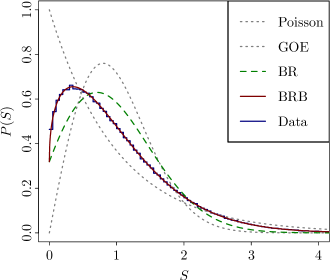
Figure 1: Nearest levels spacings distribution for $\lambda=0.15$ billiard around $k\approx 2000$. The BRB distribution fits data very well. The classical $\rho_{r}=0.175$ was used and $\beta=0.45$ was obtained from the fitting.

The open question is how does the parameter $\beta$ depend on the localization. This question was raised for the first time by Izrailev Izrailev (1988, 1989, 1990), where he numerically studied the quantum kicked rotator, which is a 1D time-periodic system. His result showed that the parameter $\beta$, which was obtained using the Izrailev distribution, is functionally related to the localization measure defined as the information entropy of the eigenstates in the angular momentum representation. His results were recently confirmed and extended, with the much greater numerical accuracy and statistical significance Manos and Robnik (2013); Batistić et al. (2013).

In this paper we show for the first time that there is indeed a functional relation between the level repulsion parameter $\beta$ and the localization measure also in autonomous quantum systems, in perfect analogy with the quantum kicked rotator. We define two different general localization measures in terms of the Husimi functions and show that they are equivalent. Our approach is quite general, but will be demonstrated in the case of the billiards as model systems.

II Localization measures

The Wigner functions, defined in the phase space $(q,p)$, have been introduced by Wigner in 1932 Wigner (1932). They are real valued, but not positive definite. Usually they oscillate around the zero value in regions which do not have much physical significance and obscure the picture, so one would prefer to smooth out such fluctutations. The Husimi functions Husimi (1940), also called Husimi quasi-probability distributions, however, are positive definite. They are defined as Gaussian smoothed Wigner functions, or equivalently, as a square of the projection of the eigenfunction of the corresponding eigenstate onto a coherent state. For definitions see e.g. reference Takahashi (1989).

We define two general localization measures in terms of the Husimi quasi-probability distribution $H(q,p)$ in a phase space, which can be computed for any quantal physical system. They are normalized, $\int dqdp\,H(q,p)=1$.

The first localization measure is the effective volume $A$ on the classical chaotic domain, covered by the Husimi function. $A$ is defined as

$$A=\frac{e^{\left<I\right>}}{\Omega_{c}}$$ (2)

where

$$I=-\int dq\,dp\,H(q,p)\log{H(q,p)}$$ (3)

is the information entropy, $\langle I\rangle$ is its average over the large number of consecutive chaotic eigenstates and $\Omega_{c}$ is the phase space volume of the chaotic domain on which $H(q,p)$ is defined. Clearly, in the case of the uniform distribution $H(q,p)=1/\Omega_{c}$, the localization measure is $A=1$, whilst in the case of the strongest localization (in a single Planck cell) $I=\log(2\pi\hbar)^{f}$, $A=(2\pi\hbar)^{f}/\Omega_{c}=1/N_{C}(E)\approx 0$, where $f$ is the number of degrees of freedom, i.e. the dimension of the configuration space, and $N_{C}(E)$ is the number of chaotic levels in the chaotic region at the energy $E$. In the semiclassical limit $2\pi\hbar\rightarrow 0$ this number is very large and thus $A\approx 0$.

For the definition of the second localization measure we first define a correlation matrix

$$C_{nm}=\frac{1}{Q_{n}\,Q_{m}}\int dq\,dp\,H_{n}(q,p)\,H_{m}(q,p)$$ (4)

where

$$Q_{n}=\sqrt{\int dq\,dp\,H_{n}^{2}(q,p)}$$ (5)

are the normalization factors and where $n$ and $m$ are just the eigenstate labels (quantum numbers). It is clear that if two Husimi functions, $H^{n}$ and $H^{m}$ do not ”live” in the same part of the phase space, their matrix element $C_{nm}$ is zero. This is possible, if the corresponding eigenstates are from the different invariant domains, or if the eigenstates are nonoverlapping on the chaotic region. The correlation matrix is therefore a useful object to study the clustering of eigenstates on the chaotic domain. Thus we define the second measure of localization $C$ as an average of $C_{nm}$ over the sufficiently large number of consecutive chaotic eigenstates

$$C=\left<C_{nm}\right>.$$ (6)

Very interestingly and surprisingly, the numerical computations, explained in the next section, show that these two localization measures are linearly proportional and thus equivalent.

III The model billiard system

Billiards are nontrivial and generic dynamical systems in which it is possible to compute a great number of high quality high lying energy levels, using many elegant numerical techniques Veble et al. (2007), especially the plane wave decomposition method Vergini and Saraceno (1995), all of them used in Batistić and Robnik (2010). We choose the family of billiards introduced by Robnik Robnik (1983, 1984), defined as the quadratic conformal map $w=z+\lambda z^{2}$ of the unit circle $|z|=1$ from the complex $z$-plane onto the physical $w$-complex plane, and study numerically a series of shapes at various $\lambda$. By varying the parameter $\lambda$ from $0$ to $1/2$ we see the transition from an integrable (circle) to the fully chaotic system Markarian (1993), which is ergodic, mixing and K. In between the system is of the mixed-type with coexisting regular and chaotic regions, a typical KAM-scenario, for $\lambda\geq 0.135$ having only one dominant chaotic region, so that smaller chaotic regions can be neglected. It has been already shown that the BRB distribution gives an excellent description of the level spacing distribution Batistić and Robnik (2010). One example is shown in figure 1. Moreover, very recently Batistić and Robnik (2013); Batistić et al. (2013) it has been explicitly demonstrated in the case of $\lambda=0.15$, with great accuracy and statistical significance ($\sim 590.000$ consecutive eigenstates), that the regular and chaotic eigenstates and the corresponding energy levels can be separated, by means of Poincaré Husimi functions, clearly yielding the Poisson statistics for the regular and Brody level spacing distribution for the chaotic eigenstates.

In order to study the localization effects and their relationship to $\beta$, we have explored a series of billiards with various values $\lambda=$ $0.135$, $0.14$, $0.145$, $0.15$, $0.155$, $0.16$, $0.165$, $0.175$, $0.18$, $0.19$, $0.2$, $0.21$, $0.22$, $0.23$, $0.24$. We have solved numerically the Helmholtz equation $\Delta\psi+k^{2}\psi=0$, with the Dirichlet boundary conditions $\psi=0$ for each $\lambda$. The size of the chaotic component $\rho_{c}$ (the relative phase space volume of the chaotic region, not to be confused with the area of the chaotic region on the Poincaré surface of section) and the degree of chaos increase monotonically with $\lambda$. The ratio $\alpha=t_{H}/t_{T}$ of the Heisenberg time $t_{H}$ and the transport time $t_{T}$ is calculated as $\alpha=2k/N_{T}$, where $N_{T}$ is the characteristic transport time in units of mean free flight time, i.e. it is the number of collisions necessary for the global classical transport. The dimensionless Heisenberg time is equal to $2k$. For example, for $\lambda=0.15$ it turns out that $N_{T}\approx 10^{5}$. If $\alpha<1$, the quantum localization occurs. See Batistić and Robnik (2013) for details. The billiards at different $\lambda$ have different transport times $N_{T}$ on the largest (dominant) chaotic component, and thus there is a different degree of localization at fixed $k$. The details of the estimates of $N_{T}$ are given in the appendix A. We have calculated the localization measures for all billiards at two different $k$, $k\approx 2000$ and $k\approx 4000$, and also the corresponding $\beta$.

We now define the localization measures in terms of the positive definite Husimi function, which is interpreted as a probability distribution of a quantum state in the phase space, and is defined below.

The classical billiard dynamics is described completely by the bounce map, using the Poincaré Birkhoff coordinates $(q,p)$. Thus it is reasonable to use the Poincaré Husimi function which is a quasi-probability distribution in the Poincaré Birkhoff phase space Bäcker et al. (2004); Batistić and Robnik (2013), defined as

$$H(q,p)=\left|\int_{\partial{\cal B}}c_{(q,p),k_{n}}(s)\,u_{n}(s)ds\right|^{2},$$ (7)

where $u_{n}(s)=\mathbf{n}(s).\nabla\psi_{n}(\mathbf{r}(s))$ is the normal derivative of the eigenfunction $\psi_{n}$ on the boundary, with ${\bf n}(s)$ being the unit outward vector to the boundary $\partial{\cal B}$ at position $s$. It is called also the boundary function, because it uniquely determines the wave function at any point inside the billiard. For details see Batistić and Robnik (2013). Here

$$c_{(q,p),k}=\sum_{m\in\mathbb{Z}}e^{ikp(s-q+mL)}\,e^{-k(s-q+mL)^{2}/2}$$ (8)

is the coherent state on the boundary (obviously periodized, thus satisfying the periodic boundary condition in $s$), centered at $(q,p)$. There is indeed no loss of information with this representation as the boundary function $u_{n}(s)$ gives the complete description of the eigenfunction in the interior of the billiard ${\cal B}$.

$H(q,p)$ has been calculated on the equidistant $400\times 400$ grid $(q_{i},p_{j})=\left(\Delta{q}/2+i\,\Delta{q},\Delta{p}/2+j\,\Delta{p}\right)$ where $\Delta{q}=L/800$ and $\Delta{p}=1/400$. The grid covers the quadrant $q\in[0,L/2]$ and $p\in[0,1]$, which remains after the reduction of the phase space due to the time reversal and the reflection symmetries. The grid points are positioned at the centers of the square cells, of the area $\Delta{q}\,\Delta{p}$. The integration method used to evaluate (7) is a simple trapeze rule with the step $ds\propto\lambda_{B}/20$, where $\lambda_{B}=2\pi/k$ is the de Broglie wavelength. Importantly, the values of the Poincaré Husimi function on the grid $H_{ij}=H(q_{i},p_{j})$ are rescaled such that their sum equals one (normalization of $H$). Two examples of the localized chaotic eigenstates are shown in figure 2.

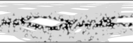
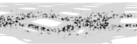
Figure 2: Poincaré Husimi functions for similar eigenstates of the $\lambda=0.15$ billiard at $k\approx 2000$ (top) and $k\approx 4000$ (bottom), showing the localization effect. The shaded area is the classical chaotic domain, which would be completely covered by the extended states in a deep semiclassical limit. Unshaded area represents the domains of regular motion.

In order to separate the regular and chaotic eigenstates we have introduced the overlap index $M$, following our previous work Batistić and Robnik (2013); Batistić et al. (2013). Each cell is ascribed the number $\gamma_{ij}$, which is either $+1$ if it belongs to the chaotic region, or $-1$ if the region is regular. These numbers are calculated classically by means of a very long chaotic orbit (about $10^{9}$ collisions). For a cell to be classified as chaotic only one visit of the chaotic orbit is sufficient. The overlap index as the classification measure is defined as the sum $M=\sum_{ij}H_{ij}\gamma_{ij}$. Ideally, if $M=+1$, the level is labeled chaotic and if $M=-1$ the level is labeled regular. Using $M$ it is possible to extract chaotic states.

We express the localization measures in terms of the discretized Husimi function. For $A$ we write

$$A=\frac{e^{\left<I\right>}}{N_{c}}$$ (9)

where

$$I=-\sum_{ij}H_{ij}\,\log{H_{ij}}$$ (10)

and $N_{c}$ is a number of cells on the classical chaotic domain. Again, in the case of uniform dsitribution $H_{ij}=1/N_{C}$ the localization measure is $A=1$, whilst in the case of the strongest localization $I=0$, and $A=1/N_{C}\approx 0$. The mean $\left<I\right>$ is obtained by averaging $I$ over a sufficiently large number of consecutive chaotic eigenstates.

The correlation matrix equals

$$C_{nm}=\frac{1}{Q_{n}\,Q_{m}}\sum_{ij}H^{n}_{ij}\,H^{m}_{ij},$$ (11)

where

$$Q_{n}=\sqrt{\sum_{ij}(H^{n}_{ij})^{2}}$$ (12)

is the normalizing factor.

For a good approximation of the localization measures $A$ and $C$ it was sufficient to separate and extract about $1.500$ consecutive chaotic eigenstates. It is very interesting and satisfying that the two localization measures are linearly equivalent as shown in figure 3. But to get a good estimate of $\beta$ we need much more levels, and the separation of eigenstates is then technically too demanding. We have instead calculated spectra on small intervals around $k\approx 2000$ and $k\approx 4000$ taking not less than $100.000$ consecutive levels (no separation) and fitted their level spacing distribution with the BRB distribution with the $\beta$ as the only fit parameter, while using the fixed classically calculated parameter $\rho_{r}$. The dependence of $\beta$ on $A$ is shown in figure 4. For aesthetic reasons we have rescaled the measure $A\rightarrow A/A_{\textrm{\small max}}$ such that it goes from 0 to 1. The maximal value of $A$, $A_{\textrm{\small max}}=0.68$, was estimated as $A_{\textrm{\small max}}=e^{I_{\textrm{\tiny max}}}/N_{c}$, where $I_{\textrm{\small max}}$ is the maximum entropy of $1500$ consecutive states of the almost fully chaotic $\lambda=0.25$ billiard. This is some kind of renormalization of $A$, such that for fully chaotic systems the procedure always yields $A=1$. Namely, in real chaotic eigenstates we never reach a perfectly uniform distribution $H(q,p)$, since they always have some oscillatory structure.

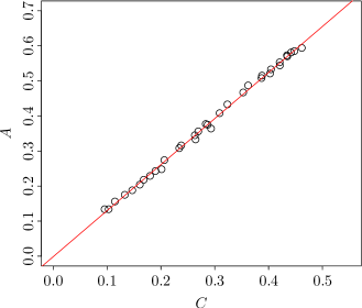
Figure 3: Linear relation between the two entirely different localization measures, namely the enrtopy measure $A$ and the correlation measure $C$, calculated for several different billiards at $k\approx 2000$ and $k\approx 4000$.

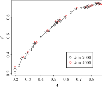
Figure 4: The central result of this letter: A clear functional relation between $\beta$ and the localization measure $A$. Arrows connect points corresponding to the same $\lambda$ at two different $k$.

We clearly see that there is a functional relationship between $A$ and $\beta$. By increasing $k$ from $2000$ to $4000$ we increase the dimensionless Heisenberg time by factor $2$, therefore the degree of localization should decrease, meaning that $A$ must increase, but precisely in such a way, that the empirical points stay on the scaling curve, as it is observed and indicated by the arrows.

Unfortunately, it is too early to propose a semiempirical functional description of the relationship we found in figure 4. In the quantum kicked rotator it is just almost linear Izrailev (1990); Manos and Robnik (2013); Batistić et al. (2013). Also, there is a great lack in theoretical understanding of its physical origin, even in the case of (the long standing research on) the quantum kicked rotator, except for the intuitive idea, that energy spectral properties should be only a function of the degree of localization, because the localization gradually decouples the energy eigenstates and levels, switching the linear level repulsion $\beta=1$ (of fully extended chaotic states) to a power law level repulsion with exponent $\beta<1$. The full physical explanation is open for the future.

IV Conclusions

Our main conclusion is that in autonomous Hamilton systems in quantum chaos the spectral level repulsion parameter of the chaotic eigenstates is functionally related to a localization measure. In our method we have defined two localization measures, one in terms of the information entropy, and the other one in terms of the correlation properties of Husimi functions. Although different by definitions, we show in the case of the billiard systems Robnik (1983, 1984), working with the Poincaré Husimi functions, that they are linearly proportional and thus equivalent. Our results are in complete analogy with the quantum kicked rotator. Further theoretical work is in progress. Beyond the billiard systems, there are many important applications in various physical systems, like e.g. in hydrogen atom in strong magnetic field Robnik (1981, 1982); Hasegawa et al. (1989); Wintgen and Friedrich (1989); Ruder et al. (1994), which is a paradigm of stationary quantum chaos, or e.g. in microwave resonators, the experiments introduced by Stöckmann around 1990 and intensely further developed since then Stöckmann (1999).

V Acknowledgement

This work was supported by the Slovenian Research Agency (ARRS).

Appendix A: Classical transport times

Here we calculate the Heisenberg time and the classical transport time for a chaotic billiard. According to the leading order of the Weyl formula, which is in fact just the simple Thomas-Fermi rule, we have for the number of levels $N(E)$ below and up to the energy $E$ of a Hamiltonian $H({\bf q},{\bf p})$

$$N(E)=\frac{1}{(2\pi\hbar)^{2}}\int_{H({\bf q},{\bf p})\leq E}d^{2}{\bf q}\;d^{2}{\bf p}.$$ (13)

Since $H={\bf p}^{2}/(2m)$, with constant zero potential energy inside ${\cal B}$, where $m$ is the mass of the billiard point particle, and $H$ is infinite on the boundary $\partial{\cal B}$, we get at once

$$N(E)=\frac{2\pi{\cal A}mE}{(2\pi\hbar)^{2}}.$$ (14)

Here ${\cal A}$ is the area of the billiard ${\cal B}$. The density of levels is $\rho(E)=1/(\Delta E)=dN(E)/dE={\cal A}m/(2\pi\hbar^{2})$ and thus the Heisenberg time is

$$t_{H}=2\pi\hbar\rho(E)=\frac{{\cal A}m}{\hbar}.$$ (15)

The classical transport time is denoted by $t_{T}$, and in units of the number of collisions $N_{T}$ can be written as

$$t_{T}=\frac{\bar{l}N_{T}}{v}=\frac{\bar{l}N_{T}}{\sqrt{2E/m}},$$ (16)

where $\bar{l}$ is the mean free path of the billiard particle and $v=\sqrt{2E/m}$ is its speed at the energy $E$. Thus for the ratio $\alpha=t_{H}/t_{T}$ we get

$$\alpha=\frac{t_{H}}{t_{T}}=\frac{{\cal A}k}{N_{T}\bar{l}}$$ (17)

where $k=\sqrt{2mE/\hbar^{2}}$. Taking into account that $\bar{l}\approx\pi{\cal A}/{\cal L}$ (this is so-called Santalo’s formula, see e.g. Santaló and Kac (2004)), we have

$$\alpha=\frac{t_{H}}{t_{T}}=\frac{{\cal L}k}{\pi N_{T}},$$ (18)

where ${\cal L}$ is the length of the perimeter $\partial{\cal B}$. This is a general formula valid for any chaotic billiard. In the case of Robnik billiards Robnik (1983, 1984) ${\cal L}\approx 2\pi$ and we arrive at the final estimate

$$\alpha=\frac{2k}{N_{T}}.$$ (19)

Thus the condition for the occurrence of dynamical localization $\alpha\leq 1$ is now expressed in the inequality

$$k\leq\frac{N_{T}}{2}.$$ (20)

Some examples of chaotic spreading of an inital ensemble of orbits placed at $p=0$ on the chaotic region are shown in figure 5, where we plot the mean square of the momentum as a function of the number of collisions, for three different values of $\lambda$.

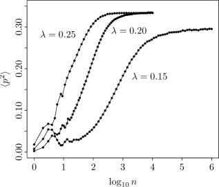
Figure 5: We show the second moment $\langle p^{2}\rangle$ averaged over an ensemble of $10^{6}$ initial conditions uniformly distributed in the chaotic component on the interval $s\in[0,{\cal L}/2]$ and $p=0$ as a function of the decadic logarithm of the number of collisions $n$. We see that the saturation value of $\langle p^{2}\rangle$ is reached at about $N_{T}=10^{5}$ collisions for $\lambda=0.15$, $N_{T}=10^{3}$ collisions for $\lambda=0.20$ and $N_{T}=10^{2}$ for $\lambda=0.25$. For $\lambda=0.15$, according to the criterion (20) at $k=2000$ and $k=4000$ we are still in the regime where the dynamical localization is expected. On the other hand, for $\lambda=0.20,0.25$ we expect extended states already at $k<2000$.

References

- Stöckmann (1999) H.-J. Stöckmann, Quantum Chaos - An Introduction (Cambridge: Cambridge University Press, 1999).
- Haake (2001) F. Haake, Quantum Signatures of Chaos (Berlin: Springer, 2001).
- Casati et al. (1979) G. Casati, B. V. Chirikov, F. M. Izrailev, and J. Ford, Lecture Notes in Physics 93, 334 (1979).
- Chirikov et al. (1981) B. V. Chirikov, F. M. Izrailev, and D. L. Shepelyansky, Sov. Sci. Rev. C 2, 209 (1981).
- Chirikov et al. (1988) B. V. Chirikov, F. M. Izrailev, and D. L. Shepelyansky, Physica D 33, 77 (1988).
- Izrailev (1990) F. M. Izrailev, Phys. Rep. 196, 299 (1990).
- Izrailev (1988) F. M. Izrailev, Phys. Lett. A 134, 13 (1988).
- Izrailev (1989) F. M. Izrailev, J. Phys. A: Math. Gen. 22, 865 (1989).
- Fishman et al. (1982) S. Fishman, D. R. Grempel, and R. E. Prange, Phys. Rev. Lett. 49, 509 (1982).
- Prosen (2000) T. Prosen, in Proc. of the Int. School in Phys. ”Enrico Fermi”, Course CXLIII, Eds. G. Casati and U. Smilansky (Amsterdam: IOS Press, 2000).
- Mehta (1991) M. L. Mehta, Random Matrices (Boston: Academic Press, 1991).
- Guhr et al. (1998) T. Guhr, A. Müller-Groeling, and H. Weidenmüller, Phys. Rep. 299, 4 (1998).
- Robnik (1998) M. Robnik, Nonl. Phen. in Compl. Syst. (Minsk) 1, 1 (1998).
- Percival (1973) I. C. Percival, J. Phys B: At. Mol. Phys. 6, L229 (1973).
- Berry and Robnik (1984) M. V. Berry and M. Robnik, J. Phys. A: Math. Gen. 17, 2413 (1984).
- Batistić and Robnik (2010) B. Batistić and M. Robnik, J. Phys. A: Math. Theor. 43, 215101 (2010).
- Batistić and Robnik (2013) B. Batistić and M. Robnik, J. Phys. A:Math. Theor. 46 (2013).
- Casati et al. (1980) G. Casati, F. Valz-Gris, and I. Guarneri, Lett. Nuovo Cimento 28, 279 (1980).
- Bohigas et al. (1984) O. Bohigas, M. J. Giannoni, and C. Schmit, Phys. Rev. Lett. 52, 1 (1984).
- Sieber and Richter (2001) M. Sieber and K. Richter, Phys. Scr. T90, 128 (2001).
- Müller et al. (2004) S. Müller, S. Heusler, P. Braun, F. Haake, and A. Altland, Phys. Rev. Lett. 93, 014103 (2004).
- Heusler et al. (2004) S. Heusler, S. Müller, P. Braun, and F. Haake, J. Phys.A: Math. Gen. 37, L31 (2004).
- Müller et al. (2005) S. Müller, S. Heusler, P. Braun, F. Haake, and A. Altland, Phys. Rev. E 72, 046207 (2005).
- Müller et al. (2009) S. Müller, S. Heusler, A. Altland, P. Braun, and F. Haake, New J. of Phys. 11, 103025 (2009).
- Gutzwiller (1980) M. C. Gutzwiller, Phys. Rev. Lett. 45, 150 (1980).
- Berry (1985) M. V. Berry, Proc. Roy. Soc. Lond. A 400, 229 (1985).
- Berry (1977) M. V. Berry, J. Phys. A: Math. Gen. 12, 2083 (1977).
- Robnik (1988) M. Robnik, in Atomic Spectra and Collisions in External Fields (New York: Plenum, 1988).
- Prosen and Robnik (1993) T. Prosen and M. Robnik, J. Phys. A: Math. Gen. 26, 2371 (1993).
- Prosen and Robnik (1994a) T. Prosen and M. Robnik, J. Phys. A: Math. Gen. 27, L459 (1994a).
- Prosen and Robnik (1994b) T. Prosen and M. Robnik, J. Phys. A: Math. Gen. 27, 8059 (1994b).
- Prosen and Robnik (1999) T. Prosen and M. Robnik, J. Phys. A: Math. Gen. 32, 1863 (1999).
- Prosen (1998) T. Prosen, J. Phys. A: Math. Gen. 31, 7023 (1998).
- Barnett and Betcke (2007) A. H. Barnett and T. Betcke, Chaos 17, 043125 (2007).
- Vidmar et al. (2007) G. Vidmar, H. J. Stöckmann, M. Robnik, U. Kuhl, R. Höhmann, and S. Grossmann, J. Phys. A: Math. Theor. 40, 13883 (2007).
- Brody (1973) T. A. Brody, Lett. Nuovo Cimento 7, 482 (1973).
- Brody et al. (1981) T. A. Brody, J. Flores, J. B. French, P. A. Mello, A. Pandey, and S. S. M. Wong, Rev. Mod. Phys. 53, 385 (1981).
- Manos and Robnik (2013) T. Manos and M. Robnik, Phys. Rev. E 87, 062905 (2013).
- Batistić et al. (2013) B. Batistić, T. Manos, and M. Robnik, EPL 102, 50008 (2013).
- Wigner (1932) E. Wigner, Phys. Rev. 40, 749 (1932).
- Husimi (1940) K. Husimi, Proc. Phys. Math. Soc. Jpn. 22, 264 (1940).
- Takahashi (1989) K. Takahashi, Prog. Theor. Phys. Suppl. (Kyoto) 98, 2109 (1989).
- Veble et al. (2007) G. Veble, T. Prosen, and M. Robnik, New J. Phys. 9, 15 (2007).
- Vergini and Saraceno (1995) E. Vergini and M. Saraceno, Phys. Rev. E 52, 2204 (1995).
- Robnik (1983) M. Robnik, J. Phys. A: Math. Gen. 16, 3971 (1983).
- Robnik (1984) M. Robnik, J. Phys. A: Math. Gen. 17, 1049 (1984).
- Markarian (1993) R. Markarian, Nonlinearity 6, 819 (1993).
- Bäcker et al. (2004) A. Bäcker, S. Fürstberger, and R. Schubert, Phys. Rev. E 70, 036204 (2004).
- Robnik (1981) M. Robnik, J. Phys. A: Math. Gen. 14, 3195 (1981).
- Robnik (1982) M. Robnik, J. Phys. Colloque C2 43, 29 (1982).
- Hasegawa et al. (1989) H. Hasegawa, M. Robnik, and G. Wunner, Prog. Theor. Phys. Suppl. (Kyoto) 98, 198 (1989).
- Wintgen and Friedrich (1989) D. Wintgen and H. Friedrich, Phys. Rep. 183, 38 (1989).
- Ruder et al. (1994) H. Ruder, G. Wunner, H. Herold, and F. Geyer, Atoms in Strong Magnetic Fields (Heidelberg: Springer, 1994).
- Santaló and Kac (2004) L. A. Santaló and M. Kac, Integral geometry and geometric probability, Cambridge mathematical library (Cambridge University Press, Cambridge, 2004).