Pioneers of Influence Propagation in Social Networks

Abstract

With the growing importance of corporate viral marketing campaigns on online social networks, the interest in studies of influence propagation through networks is higher than ever. In a viral marketing campaign, a firm initially targets a small set of pioneers and hopes that they would influence a sizeable fraction of the population by diffusion of influence through the network. In general, any marketing campaign might fail to go viral in the first try. As such, it would be useful to have some guide to evaluate the effectiveness of the campaign and judge whether it is worthy of further resources, and in case the campaign has potential, how to hit upon a good pioneer who can make the campaign go viral.

In this paper, we present a diffusion model developed by enriching the generalized random graph (a.k.a. configuration model) to provide insight into these questions. We offer the intuition behind the results on this model, rigorously proved in [6], and illustrate them here by taking examples of random networks having prototypical degree distributions — Poisson degree distribution, which is commonly used as a kind of benchmark, and Power Law degree distribution, which is normally used to approximate the real-world networks. On these networks, the members are assumed to have varying attitudes towards propagating the information. We analyze three cases, in particular — (1) Bernoulli transmissions, when a member influences each of its friend with probability $p$; (2) Node percolation, when a member influences all its friends with probability $p$ and none with probability $1-p$; (3) Coupon-collector transmissions, when a member randomly selects one of his friends $K$ times with replacement.

We assume that the configuration model is the closest approximation of a large online social network, when the information available about the network is very limited. The key insight offered by this study from a firm’s perspective is regarding how to evaluate the effectiveness of a marketing campaign and do cost-benefit analysis by collecting relevant statistical data from the pioneers it selects. The campaign evaluation criterion is informed by the observation that if the parameters of the underlying network and the campaign effectiveness are such that the campaign can indeed reach a significant fraction of the population, then the set of good pioneers also forms a significant fraction of the population. Therefore, in such a case, the firms can even adopt the naïve strategy of repeatedly picking and targeting some number of pioneers at random from the population. With this strategy, the probability of them picking a good pioneer will increase geometrically fast with the number of tries.

1 Introduction

Traditionally, firms had few avenues when trying to market their products. And the most important of these avenues — television, newspapers, billboards — are notoriously inflexible and inefficient from the firms’ point of view. Essentially, a firm has to pay to reach even those people who would never form a part of its target demographic ([14]). From the consumers’ point of view, they are continuously bombarded with advertisements of products, a vast majority of which do not interest them. In such a scenario, there is even a possibility that a significant fraction of consumers might just tune-off and become insensitive to every advertisement. The idea of direct marketing tried to overcome some of these problems by the construction of a database of the buying patterns and other relevent information of the population, and then targeting only those who are predisposed to get influenced by a particular marketing campaign ([12]). However, targeting the most responsive customers individually can be expensive and thus limits the reach of direct marketing. Moreover, it precludes the possibility of positive externalities such as a favorable shift in preferences of a demographic segment previously thought to be unresponsive.

The penetration of internet and the emergence of huge online social networks in the last decade has radically altered the way that people consume media and print, leading to an ongoing decline in importance of conventional channels and consequently, marketing through them. This radical shift has brought in its wake a host of opportunities as well as challenges for the advertisers. On the one hand, firms finally have the possibility to reach in a cost-effective way not only the past responsive customers, but indeed all the potentially responsive ones. The importance of this new marketing medium is witnessed by the fact that most of the big corporations, particularly those providing services or producing consumer goods, now have dedicated fan-pages on social networks to interact with their loyal customers. These, in turn, help the firms spread their new marketing campaign to a large fraction of the network, reliably and at a fraction of the cost incurred through traditional channels. On the other hand, new firms without a loyal fan-base have found it a hit-or-miss game to gain attention through the new medium. Even though the marketing through network is mostly a miss for these firms, but when it is a hit, it is a spectacular one. This makes it tempting for firms to keep waiting for that spectacular hit while their marketing budget inflates beyond the point of no return. The fat-tail uncertainty of viral marketing makes it inherently different from conventional marketing and calls for a fundamentally different approach to decision-making: which individuals, and how many, to initially target in the online network? What amount of resources to spend on these initially targeted pioneers? And most importantly, when to stop, admit the inefficacy of the current campaign and develop a new one?

1.1 Results

In this paper, we introduce a generalized diffusion dynamic on configuration model, which serves as a very useful approximation of an online social network, particularly when one does not have an access to a detailed information about the network structure. The diffusion dynamic that we study on this underlying random network is essentially this: any individual in the network influences a random subset of its neighbours, the distribution of which depends on the effectiveness of the marketing campaign.

We illustrate large-network-limit results on this model, rigorously proved in [6]. The empirical distribution of the number of friends that a person influences in the course of a marketing campaign is taken as a measure of the effectiveness of the campaign. We present a condition depending on network degree-distribution (the emperical distribution of the number of friends of a network member) and the effectiveness of a marketing campaign which, if satisfied, will allow, with a non-negligible probability, the campaign to go viral when started from a randomly chosen individual in the network. Given this condition, we present an estimate of the fraction of the population that is reached when the campaign does go viral. We then show that under the same condition, the fraction of good pioneers in the network, i.e., the individuals who if targeted initially will lead the campaign to go viral, is non-negligible as well, and we give an estimate of this fraction. We analyze in detail the process of influence propagation on configuration model having two types of degree-distribution: Poisson and Power Law. Three examples illustrating the dynamic of influence propagation on these two networks are considered: (1) Bernoulli transmissions; (2) Node percolation; (3) Coupon-collector transmissions.

Based on the above analysis, we offer a practical decision-making guide for marketing on online networks which we think would be particularly useful to firms with no prior access to detailed network structure. Specifically, we consider the naïve strategy of picking some number of pioneers at random from the population, spending some fixed amount of resources on each of them and waiting to see if the campaign goes viral, picking another batch if it does not. For this strategy, we suggest what statistical data the firm should collect from its pioneers, and based on these, how to estimate the effectiveness of the campaign and make a cost-benefit analysis.

1.2 Related Work

While the public imagination is captured by a new viral video of a relatively unknown artist, researchers have been trying to understand this phenomenon much before the emergence of online social networks. It was first studied in the context of the spread of epidemics on complex networks, whence the term viral marketing originates ([3], [13]). The impact of social network structure on the propagation of social and economic behavior has also been recognized ([5], [15]) and there is growing evidence of its importance ([4]).

In the context of viral marketing, broadly speaking, two approaches have developed in trying to exploit the network structure to maximize the probability of marketing campaign going viral for each dollar spent. The first approach tries to locate the most influential individuals in the network who can then be targeted to seed the campaign ([11]). This idea has been developed into a machine learning approach which relies on the availability of large databases containing detailed information regarding the network structure and the past instances of influence propagation to come up with the best predictor of the most influential individuals who should be targeted for future campaigns ([7]). Our approach, although fundamentally based on the analysis of the most influential network members, whom we call pioneers, differs in its philosophy of how to apply this to make marketing decisions. We do not rely on locating the pioneers by data-mining the network since the tastes of online network members shift at a rapid rate and the past can be an unreliable predictor for the current campaign. Moreover, the network database is not necessarily accessible to every firm. Therefore, we favor a strategy which enables one to gain exposure to positive fat-tail events while covering his/her back. However, since we suggest a way to measure the current campaign’s effectiveness based on its ongoing diffusion in the network, it can be used to develop better predictors even when the network information is freely accessible.

The second approach that has become popular in this context does not focus on locating influential network members but instead on giving incentives to members to act as a conduit for the diffusion of the campaign ([2]). Various mechanisms for determining the optimal incentives have been proposed and analyzed on random networks ([1]) as well as on a deterministic network ([9]). This approach can be particularly effective for web-based service providers, e.g., movie-renting business, where the non-monetary incentive of using the service freely or cheaply for some period of time can motivate people to proactively advertise to their friends. However, it is not always possible to come up with non-monetary expensive while offering monetary incentives is not cost-effective. In such cases, our approach can offer a more cost-effective alternative by leveraging the inherent tendency of a social network to percolate information without external incentives.

A variety of marketing strategies have been conceived combining the two broad approaches that we described above. We hope that our approach would enrich the spectrum and further help in understanding and exploiting the phenomenon of viral marketing.

2 Model and thoretical claims

In this section, we introduce our model and informally describe the results which are rigorously proved in [6].

2.1 Model

Consider that the only information available to you about an online social network is the number of friends that a subset of network members have, a realistic assumption if you are dealing with the biggest and the most important social networks out there. In such a case, the best you can do is to work with a uniform random network which agrees with the statistics that you can obtain from the available information. Such a uniform random network is obtained by constructing what is known as configuration model (CM); cf [16]. This random network is realized by attaching half-edges to each vertex corresponding to its degree (which represents here, the number of friends) and then uniformly pair-wise matching them to create edges. We assume this model of the social network throughout the paper and will use interchangeably the terms “social graph” and “random network” meaning precisely the CM. We call the vertices of this graph “nodes” or “users” and graph neighbours “friends”.

We consider a marketing campaign started from some initial target called pioneer in this network. The most natural propagation dynamic to assume in the absence of any other information is that a person influences a random subset of its friends who further propagate the campaign in the same manner. The number of friends that a person influences depends on a particular campaign. To model this dynamic, we enhance the configuration model by partitioning the half-edges into transmitter half-edges, those through which the influence can flow and receiver half-edges which can only receive influence. So, if a person A influences his friend B in the network, then in our representation, A has a transmitter half-edge matched to the transmitter or receiver half-edge of B.

Let $D$ and $D^{(t)}$ denote the empirically observed distributions of total degree and transmitter degree respectively. Empirical receiver degree distribution, $D^{(r)}$, is therefore $D-D^{(t)}$. Then we have the following large-network-limit results, rigorously proved in [6], but only informally stated here.

2.2 Theoretical claims

Claim 2.1

Starting from a randomly selected pioneer, the campaign can go viral, i.e., reach a strictly positive fraction of the population, with a strictly positive probability if and only if

$$\mathbb{E}[D^{(t)}D]>\mathbb{E}[D^{(t)}+D].$$ (1)

Note that $\mathbb{E}[D^{(t)}D]>\mathbb{E}[D^{(t)}+D]$ implies

$$\mathbb{E}[D(D-2)]>0$$ (2)

and recall that this latter condition is necessary and sufficient  for the existence of a (unique) connected component of the underlying social graph, called big component, encompassing a strictly positive fraction of its population; cf [10]. Obviously, our campaign can go viral only within this big component.

Call good pioneers the pioneers from which the campaign can go viral.

Claim 2.2

If (1) is satisfied then the population reached is, more or less, the same irrespective of the good pioneer chosen initially.

Let $C^{*}$ denote the population reached by the campaign when started from a good pioneer and $\overline{C}^{*}$ the set of good pioneers.

Claim 2.3

If (1) is satisfied then the set of good pioneers $\overline{C}^{*}$ also forms a strictly positive fraction of the population.

The next claim gives the estimates on the size of $C^{*}$ and $\overline{C}^{*}$. Let

$$H(x):=\mathbb{E}[D]x^{2}-\mathbb{E}[D^{(r)}]x-\mathbb{E}[D^{(t)}x^{D}]$$ (3)

and

$$\overline{H}(x):=\mathbb{E}[D]x^{2}-\mathbb{E}[D^{(t)}x^{D^{(t)}}]-\mathbb{E}[D^{(r)}x^{D^{(t)}}]x.$$ (4)

If condition (1) is satisfied then $H(x)$ and $\overline{H}(x)$ have unique zeros in $(0,1)$. Call them $\xi$ and $\overline{\xi}$ respectively. Denote also by $G_{D}(x)=\mathbb{E}[x^{D}]$ and $G_{D^{(t)}}(x)=\mathbb{E}[x^{D^{(t)}}]$ the probability generating function (pgf) of $D$ and $D^{(t)}$, respectively.

Claim 2.4

If (1) is satisfied and $n$ denotes the size of network population, then for $n$ large,

$$\frac{\left|C^{*}\right|}{n}\approx 1-G_{D}(\xi)=:\alpha>0$$ (5)

and

$$\frac{\left|\overline{C}^{*}\right|}{n}\approx 1-G_{D^{(t)}}(\bar{\xi})=:\overline{\alpha}>0.$$ (6)

Note that $\overline{\alpha}$ can be interpreted as the probability that the campaign goes viral when started from a randomly chosen pioneer.

In the Appendix we sketch the main arguments allowing to prove the above claims; see [6] for formal statements and proofs. Recall also from [10] that under assumption (2) the size $|C_{0}|$ of the big network component $C_{0}$ satisfies for $n$ large

$$\frac{\left|C_{0}\right|}{n}\approx 1-G_{D}(\xi_{0})=:\alpha_{0}>0\,,$$ (7)

where $\xi_{0}$ is the unique zero of

$$H_{0}(x):=\mathbb{E}[D]x^{2}-xG^{\prime}_{D}(x)$$

in $(0,1)$, with $G^{\prime}_{D}(x)$ denoting the derivative of the pgf of $D$.

3 Examples

Let us consider the results of Section 2 in the context of a few illustrative network examples.

3.1 Bernoulli transmissions

Let us assume some arbitrary distribution of the degree $D$ satisfying (2) (to guarantee the existence of the big component of the social graph). Suppose that each user decides independently for each of its friends with probability $p\in[0,1]$ whether to transmit the influence to him or not. We call this model CM with Bernoulli transmissions and $p$ the transmission probability. Note that given the total degree $D$, the transmitter degree $D^{t}$ is Binomial$(D,p)$ random variable.

Fact 3.1

In the CM with a general degree distribution $D$ satisfying (2) and Bernoulli transmissions, the campaign can go viral if and only if the transmission probability $p$ satisfies

$$p>\frac{\mathbb{E}[D]}{\mathbb{E}[D^{2}]-\mathbb{E}[D]}\,.$$ (8)

In this latter case the fraction of the influenced population and the fraction of good pioneers are asymptotically equal to each other $|C^{*}|/n\approx|\bar{C}^{*}|/n=:\alpha$, for large $n$, and satisfy

$$\alpha=1-G_{D}(\xi)\,,$$ (9)

where $\xi$ is the unique zero of the function

$$\mathbb{E}[D]((x-1)/p+1)-G^{\prime}_{D}(x)$$

in $(0,1)$.

Proof 3.1.

Bernoulli transmissions with (3) and (4) imply $H(x)=\mathbb{E}[D]x^{2}-(1-p)\mathbb{E}[D]x-pxG^{\prime}_{D}(x)$ and $\overline{H}(x)=\mathbb{E}[D]x^{2}-G^{\prime}_{D}(1-p(1-x))$. Moreover $\overline{G}_{D^{(t)}}(x)=G_{D}(1-p(1-x))$. Dividing $H(x)$ by $px$ and substituting $y:=1-p(1-x)$ in $\overline{H}(x)$ and $\overline{G}_{D^{(t)}}(x)$ completes the proof.

Consider two specific network degree examples.

Example 3.2 (Poisson degree).

When $D$ has Poisson distribution of parameter $\lambda$ (in which case the CM is asymptotically equivalent to the Erdös-Rényi model) the condition (8) reduces to

$$\lambda p>1$$

and the fraction of the influenced population and good pioneers (9) is equal to

$$\alpha=(1-\xi)/p\,,$$

where $\xi$ is the unique zero of the function

$$(x-1)/p+1-\exp(\lambda(x-1)$$

in $(0,1)$ .

More commonly observed degree-distributions in social networks have power-law tails.

Example 3.3 (Power-Law (“zipf”) degree).

Assume $D$ having distribution

$$\mathbb{P}\{D=k\}=k^{-\beta}/\zeta(\beta)\quad k=1,2,\ldots\,,$$

with $\beta>2$, where $\zeta(\beta)$ is the zeta function. Recall that the pgf of $D$ is equal to $G_{D}(x)=\text{Li}_{\beta}(x)/\zeta(\beta)$, where $\text{Li}_{\beta}(x)=\sum_{k=1}^{\infty}k^{-\beta}x^{k}$ is the so-called poly-logarithmic function. Condition (2) for the existence of the big component is equivalent to

$$\zeta(\beta-2)-2\zeta(\beta-1)>0\,,$$

which is approximately $\beta<3.48$. Condition (8) reduces to

$$p>\zeta(\beta-1)/(\zeta(\beta-2)-\zeta(\beta-1))$$

and the fraction of the influenced population and good pioneers (9) is equal to

$$\alpha=1-\text{Li}_{\beta}(\xi)\,,$$

where $\xi$ is the unique zero of the function

$$x\zeta(\beta-1)((x-1)/p+1)-\text{Li}_{\beta-1}(x)$$

in $(0,1)$.

Recall from Fact 3.1, that Bernoulli transmissions lead to the model where the fraction of the influenced population and the fraction of good pioneers are asymptotically equal to each other. In what follows we present two scenarios where the set of good pioneers and the influenced population have different size.

3.2 Enthusiastic and apathetic users or node percolation

Consider CM with a general degree distribution $D$ satisfying (1), whose nodes either transmit the influence to all their friends (these are “enthusiastic” nodes) or do not transmit to any of their friends (“apathetic” ones). Let $p$ denote the fraction of nodes in the network which are enthusiastic. Note that this model corresponds to the node-percolation  on the CM. Thus, in this model, given $D$, $D^{(t)}=D$ with probability $p$ and $D^{(t)}=0$ with probability $1-p$.

Fact 2.

Consider node-percolation on the CM with a general degree distribution $D$ satisfying (2). The campaign can go viral if and only if the fraction $p$ of enthusiastic users satisfies condition (3.1); the same as for the Bernoulli model. Moreover, in this case, the fraction $\alpha$ of reached population is also the same as in the network with Bernoulli transmissions, i.e., equal to (9) with $\xi$ as in Fact 3.1. However, the fraction $\overline{\alpha}$ of good pioneers is equal to $\overline{\alpha}=p\alpha$.

The proof follows easily from the general results of Section 2.2. Note that the campaign on the network with enthusiastic and apathetic users can reach the same population as in the Bernoulli transmissions, however there are less good pioneers.

3.3 Absentminded users or coupon-collector transmissions

Consider again CM with a general degree distribution $D$ satisfying (1). Suppose that each user is willing (or allowed) to transmit $K$ messages of influence. In this regard, it randomly selects $K$ times one of his friends with replacement (as if he were forgetting his previous choices). An equivalent dynamic of the influence propagation can be formulated as follows: every influenced user, at all times, keeps choosing one of its friends uniformly at random and transmits the influence to him; it stops forwarding the influence after $K$ transmissions.

In this model the transmission degree $D^{(t)}$ correspond to the number of collected coupons in the classical coupon collector problem with the number of coupons being the vertex degree $D$ and the number of trials $K$. The conditional distribution of $D^{(t)}$ given $D$ can be expressed as follows:

$$\mathbb{P}\{\,D^{(t)}=k\,|\,D\,\}=\frac{D!}{(D-k)!D^{-K}}\Bigl{\{}{K\atop k}\Bigr{\}}\,,$$

where $\{{K\atop k}\}=1/k!\sum_{i=0}^{K}(-1)^{i}{k\choose i}(k-i)^{K}$ is the Stirling number of the second kind.

Calculating the pgf for this distribution is tedious and we do not present analytical results regarding this model but only simulations and estimation. As we shall see in Section 3.4, in this model the influenced population is smaller than the population of good pioneers.

3.4 Numerical examples

We will present now a few numerical examples of networks and diffusion models presented above.

3.4.1 Simulations

In all our examples we simulate the enhanced configuration model on $N=1000$ nodes assuming some particular node degree $D$ distribution and influence propagation mechanism modeled by the conditional distribution of the transmitter degree $D^{(t)}$. More precisely, we sample the individual node degrees and transmitter degrees $(D_{i},D_{i}^{(t)})$ $i=1\,...\,N$ independently from the joint distribution of $(D,D^{(t)})$ and use these values to construct an instance of our enhanced CM by uniform pairwise matching of the half-edges. We calculate the relative size of the influenced population and the set of good pioneers through the exploration of the influenced components for all nodes.  In fact, relative sizes of the populations reached from different pioneers concentrate very clearly, as shown on Figure 1, which illustrates the statement of Claim 2.1.

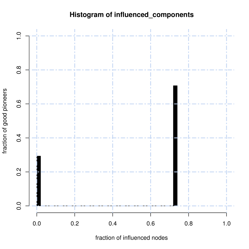
Figure 1: Concentration of the relative sizes of populations reached from different pioneers. CM with Poisson degree of mean $\lambda=2$ and Bernoulli transmissions with $p=0.8$.

3.4.2 Estimation

We adopt also the following “semi-analytic” approach: Using the sample $(D_{i},D_{i}^{(t)})$, $i=1,\ldots,N$ used to construct the CM, we consider estimators

$$\hat{G}_{D}(x) :=\frac{1}{N}\sum_{i=1}^{N}x^{D_{i}}$$ (10)

$$\hat{G}_{D}^{(t)}(x) :=\frac{1}{N}\sum_{i=1}^{N}x^{D_{i}^{(t)}}$$ (11)

$$\hat{H}(x) :=\frac{1}{N}\sum_{i=1}^{N}\Bigl{(}D_{i}x^{2}-(D_{i}-D_{i}^{(t)})x-D_{i}^{(t)}x^{D_{i}}\Bigr{)}$$ (12)

$$\hat{\overline{H}}(x) :=\sum_{i=1}^{N}\Bigl{(}D_{i}x^{2}-D_{i}^{(t)}x^{D_{i}^{(t)}}-(D_{i}-D_{i}^{(t)})x^{D_{i}^{(t)}+1}\Bigr{)}\,$$ (13)

of the functions $G_{D}(x)$, $G_{D^{(t)}}(x)$, $H(x)$ and $\overline{H}(x)$, respectively. We calculate estimators $\hat{\alpha}$ and $\hat{\overline{\alpha}}$ of the fraction of the influenced population $\alpha$ and of good pioneers $\overline{\alpha}$ using Claim 5 and the estimated functions $\hat{G}_{D}(x)$, $\hat{G}_{D^{(t)}}(x)$, $\hat{H}(x)$ and $\hat{\overline{H}}(x)$. (That is, we find numerically zeros $\hat{\xi}$ and $\hat{\overline{\xi}}$ of $\hat{H}(x)$ and $\hat{\overline{H}}(x)$, respectively, and plug them into (5) and (6), with $\hat{G}_{D}(x)$ and $\hat{G}_{D^{(t)}}(x)$ replacing $G_{D}(x)$ and $G_{D^{(t)}}(x)$.)

Note that in the semi-analytic approach we do not need to know/construct the realization of the underlying model. This observation is a basis of a campaign evaluation method that we propose in Section 4. In fact, in reality one usually does not have the complete insight into the network structure and needs to rely on statistics collected from the initially contacted pioneers.

3.4.3 Analytic evaluation

Finally, for all models, except the “coupon-collector” one of Section 3.3, we calculate numerically the values of $\alpha$ and $\overline{\alpha}$ using the explicit forms of all the involved functions. (For the coupon-collector model we obtained the “true” values of $\alpha$ and $\overline{\alpha}$ from a sample of $(D_{i},D_{i}^{(t)})$ of a larger size $N$.)

When comparing these analytic solutions to the simulation and semi-analytic estimates we see that in some cases $N=1000$ is not big enough to match the theoretical values. One can easily consider larger samples, however we decided to stay with $N=1000$ to show how the quality of the estimation varies over different model assumptions. Also, $N=1000$ seems to be near the lower range of the number of initial pioneers one needs to contact to produce a reasonable prognosis for the development of the campaign.

3.4.4 Case study

Figures 2 and 3 present Bernoulli influence propagation on the CM with Poisson and Power-Law degree distribution of mean $\mathbb{E}[D]=2,\,4,\,6$. Bernoulli transmissions imply the set of good pioneers and influenced population of the same size. The Power-Law degree with $\beta<3$ leads to positive fraction of good pioneers and influenced component for all $p>0$, while for the Poisson degree distribution one observes the phase transition at $p=1/\lambda$. That is, the fractions of good pioneers and the influenced component are strictly positive if and only if $p>1/\lambda$.

Figure 4 shows again the model with Bernoulli transmissions on CM with Poisson and Power-Law degree distribution, this time however for $\mathbb{E}[D]\approx 1.35$ for which both models exhibit the phase transition in $p$.

A general observation is that the Power-Law degree distribution gives smaller critical values of $p$ for the existence of a positive fraction of influenced population and good pioneers, however for these the size of these sets increase with the transmission probability $p$ more slowly in the Bernoulli model. Obviously the values of $\alpha=\overline{\alpha}$ at $p=1$ correspond to the size of the biggest connected component of the underlying CM.

Figure 5 shows the node percolation (or “apathetic and enthusiastic users) on CM with Poisson and Power-Law degree distribution of mean $\mathbb{E}[D]\approx 2$. Note that the influenced components have the same size as for Bernoulli transmissions, however good components are smaller. The critical values of $p$ for the phase transition are also the same as for Bernoulli transitions. Note that estimation of the node percolation model is more difficult than the Bernoulli transmissions because of higher variance of the estimators.

Finally, Figure 6 shows that the coupon collector dynamics (“absentminded users”) on CM produces bigger sets of good pioneers than the influenced population.

4 Application to Viral Campaign Evaluation

What does the analysis presented up to now suggest in terms of strategy for a firm which is just about to start a new marketing campaign on an online social network without having any prior information about the network structure?

If the fraction of good pioneers in the network is non-negligible, the firm has a strictly positive probability of picking a good pioneer even when it picks a pioneer uniformly at random from the network. Now when is the fraction of good pioneers non-negligible? Since the firm has no prior information about the network structure and the campaign effectiveness, the best it can do is to collect information from its pioneers regarding the number of friends that they have (total degree) and the number of friends they influence in this campaign (transmitter degree), and then assume that the network is a uniform random network having the sampled total degree and transmitter degree distributions. The collected information, denote it by $(D_{i},D_{i}^{(t)})$, $i=1,\ldots,N$, allows to estimate various quantities relevant to the potential development of the ongoing campaign, as we did in 3.4.

More precisely the results presented in Section 2.2 suggest the following approach.

Network fragmentation

The first and foremost question is whether the network is not too fragmented to allow for viral marketing. This is related to condition (2). In order to answer this question one considers the following estimator of $\mathbb{E}[D^{2}-2D]$

$$\frac{1}{N}\sum_{i=1}^{N}\Bigl{(}D_{i}^{2}-2D_{i}\Bigr{)}\,.$$

If the value of this estimator is not sharply larger than zero then the firm must assume that the network is too fragmented to allow for viral marketing. Natural confidence intervals can be considered in this context too. Evidently, the confidence increase as the firm picks more pioneers and collects more data.

Effectiveness of the campaign

If one estimates that the network is not too fragmented, then the firm can evaluate the effectiveness of the ongoing campaign. It is related to condition (1). Again one considers the natural estimate of $\mathbb{E}[DD^{(t)}-D^{(t)}-D]$

$$\frac{1}{N}\sum_{i=1}^{N}\Bigl{(}D_{i}D_{i}^{(t)}-D_{i}-D_{i}^{(t)}\Bigr{)}\,.$$

If the value of this estimator is sharply larger than zero then the firm can assume that there is a realistic chance of picking a good pioneer via random sampling and make the campaign go viral. Otherwise, the previous phase of the campaign can be considered as non-efficient.

Cost-benefit analysis

If the firm deems the campaign to be effective, it can then, exactly as we did in 3.4.2, come up with the estimates of the relative fractions of good pioneers and population vulnerable to influnce, and do a cost-benefit analysis. What we have described is an outline which can be used by the firms to come up with a rational methodology for making decisions in the context of viral marketing.

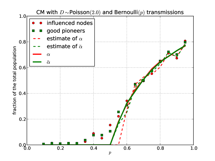
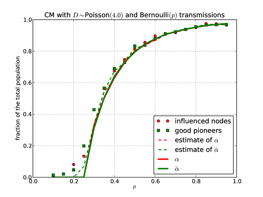
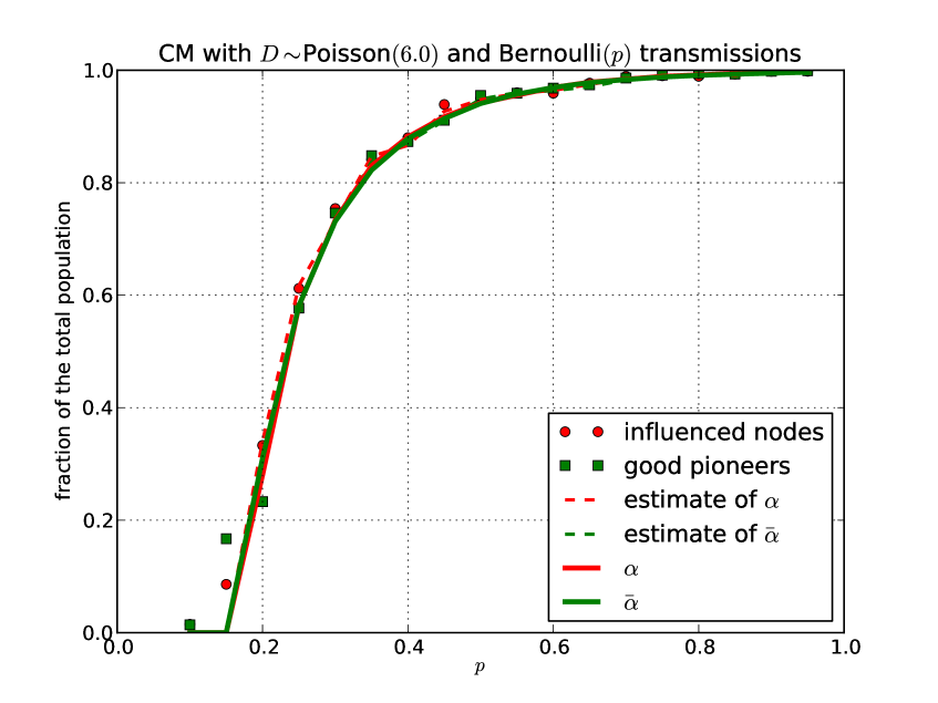
Figure 2: CM with Poisson degree of mean $\lambda=2,\,4,\,6$ and Bernoulli transmissions with probability $p$. The set of good pioneers and the influenced population are of the same size. Their fraction is strictly positive for $p>1/\lambda$.

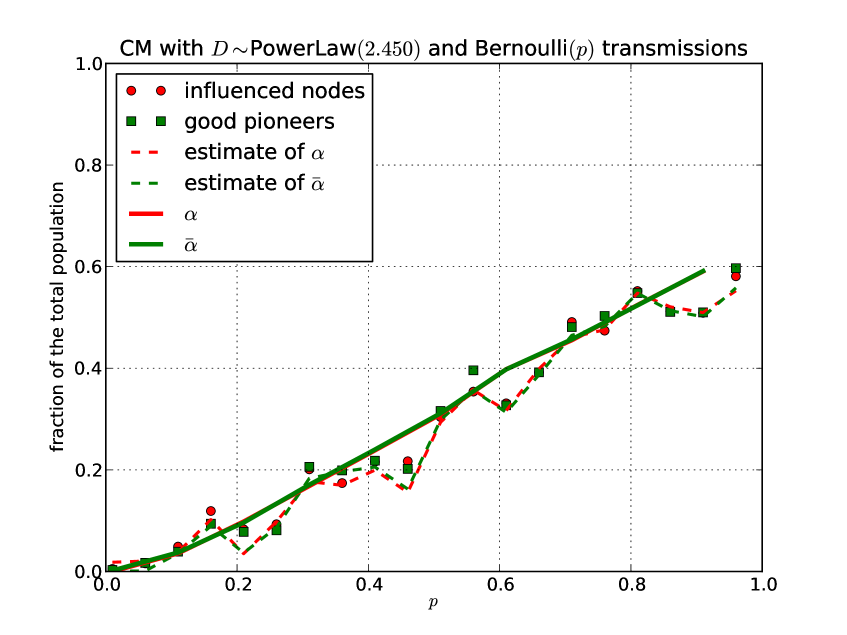
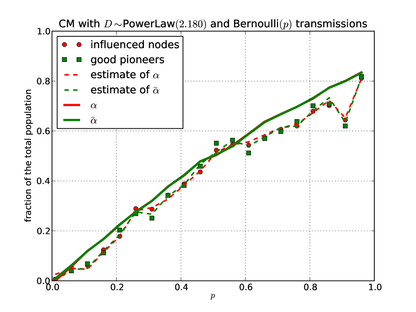
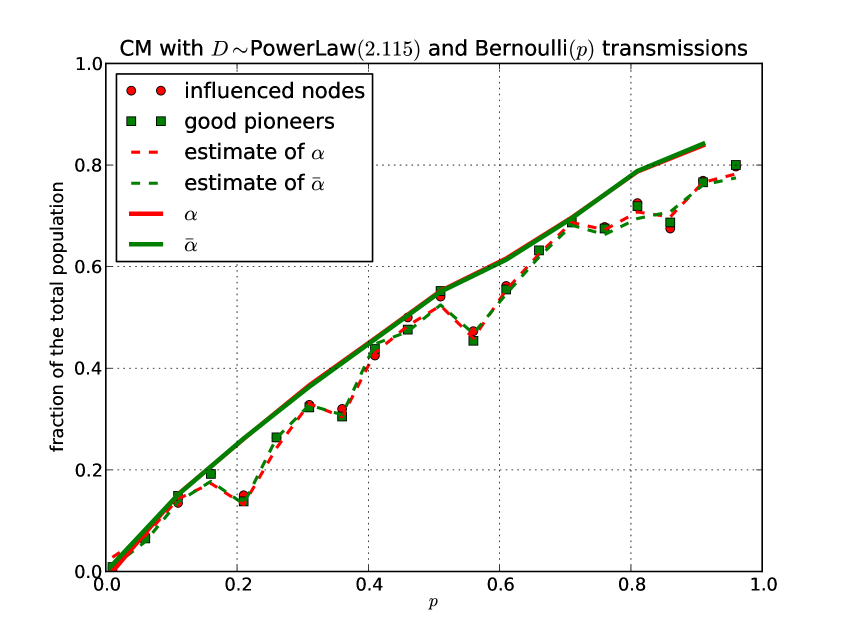
Figure 3: CM with Power-Law degree of parameter $\beta=2.450,\,2.180,\,2.115$ (corresponding to $\mathbb{E}[D]\approx 2,\,4,\,6$ and Bernoulli transmissions with probability $p$. The set of good pioneers and the influenced population are of the same size. Their fraction is strictly positive for all $p>0$ whenever $\beta\leq 3$.

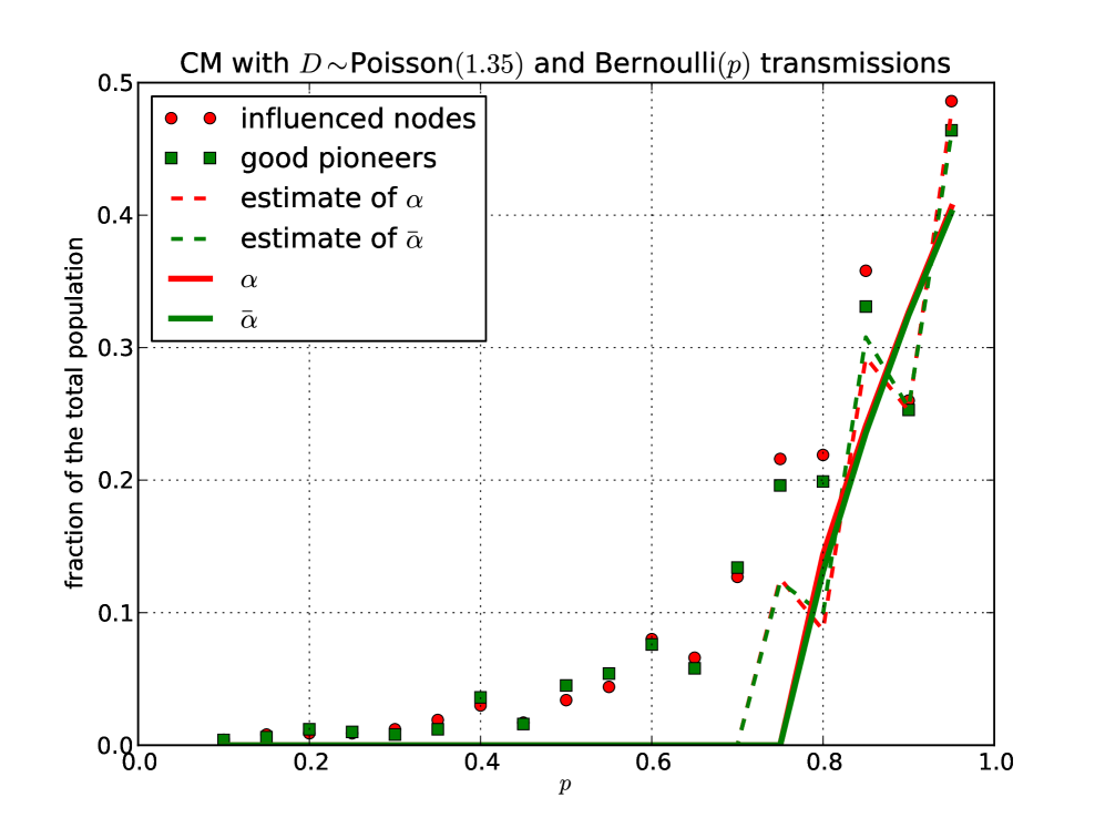
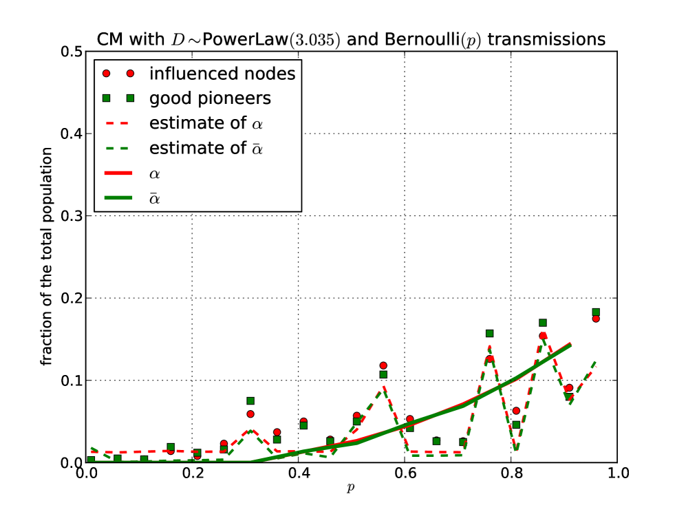
Figure 4: CM with Poisson and Power-Law degree of mean $\mathbb{E}[D]\approx 1.35$ ($\lambda=1.35$ and $\beta=3.035$) and Bernoulli transmissions. The set of good pioneers and the influenced population are of the same size for each model. One observes the phase transition in both models, at $p=1/\lambda$ and $p=\zeta(\beta-1)/(\zeta(\beta-2)-\zeta(\beta-1)$, respectively.

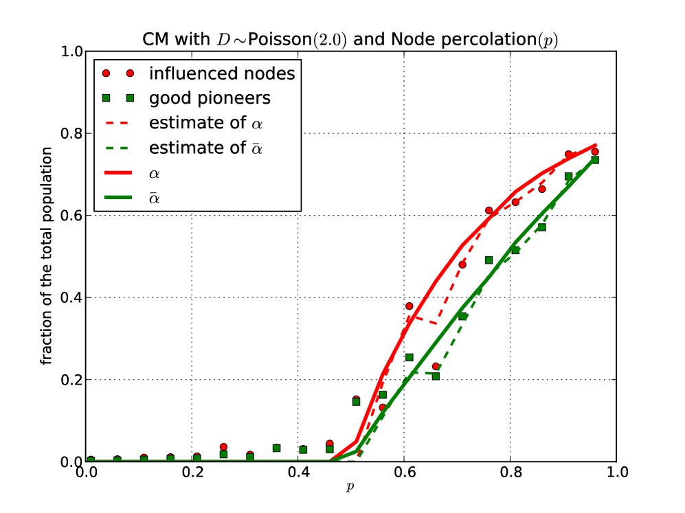
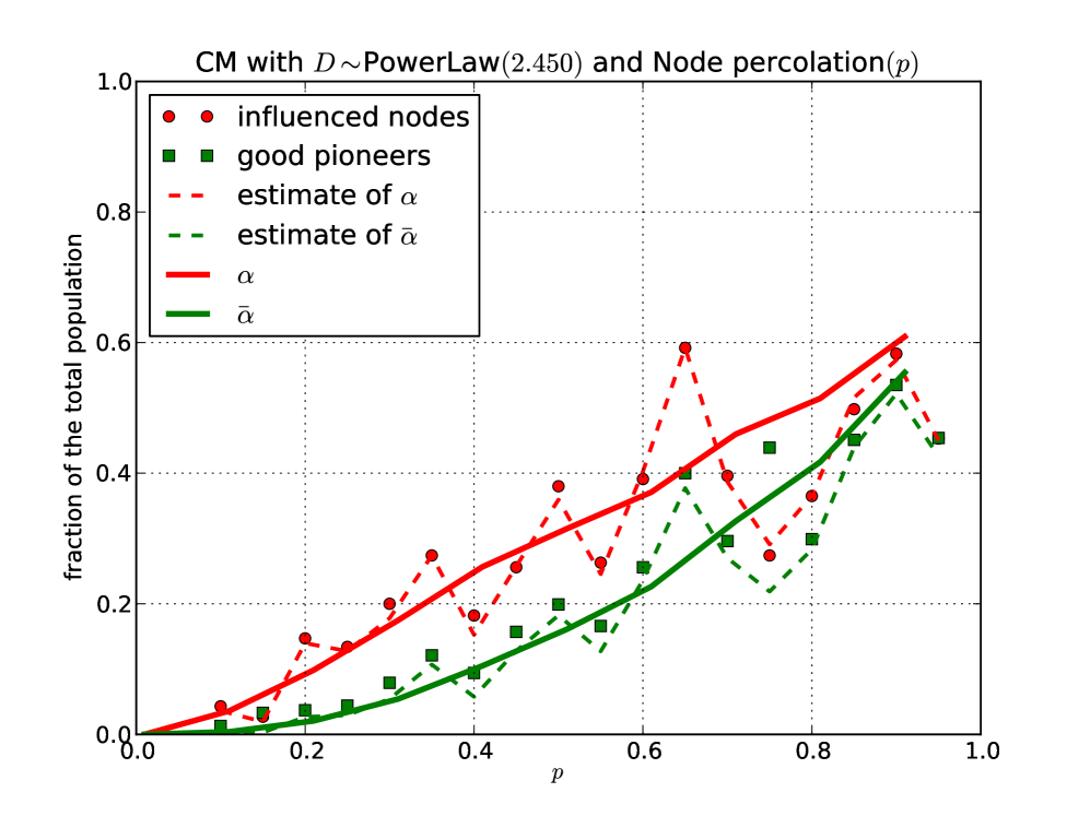
Figure 5: Node percolation (“apathetic and enthusiastic users”) on CM with Poisson and Power-Law degree of mean $\mathbb{E}[D]\approx 2$ ($\lambda=2$ and $\beta=2.45$). The influenced component and the critical values for $p$ are equal to these for the CM with Bernoulli transmissions. The set of good pioneers is smaller than the influenced population. We do not observe the phase transition for the Power-Law model since $\beta<3$.

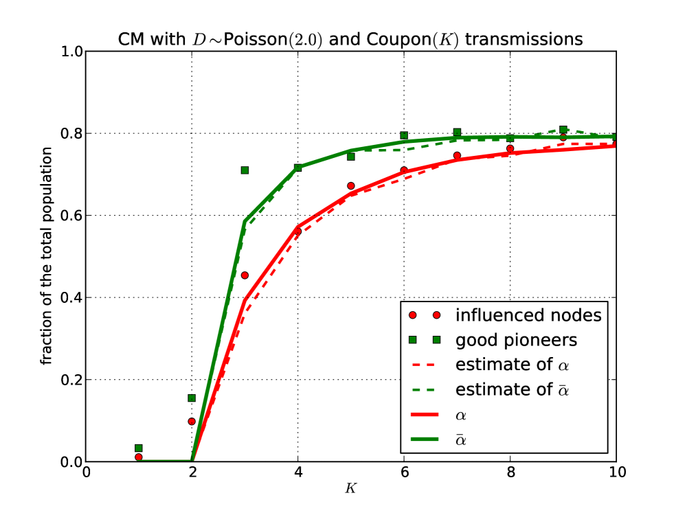
Figure 6: Coupon collector dynamics “absentminded users”) on CM with Poisson and Power-Law degree of mean $\mathbb{E}[D]\approx 2$ ($\lambda=2$ and $\beta=2.45$). The set of good pioneers is bigger than the influenced population.

5 Conclusion and Future Work

Diffusion studies on networks generally tend to focus on the component of population which is vulnerable to influence, the component that can be reached starting from an initial target. In this work, we focus on the other side of coin, i.e., the subset of population, called good pioneers, from which an initial target must be picked so that a large fraction of the population is influenced.

Our analysis of the set of good pioneers is based on a new approach proposed in [6], consisting of identifying this subset as the big component of a reverse dynamic in which an “acknowledgement” message is sent in the reversed direction on every edge thus allowing to trace all the possible sources of influence of a given vertex.

Based on the recent graph-theoretical results obtained through this approach regarding the existence and the size of both subsets: of good pioneers and vulnerable population, we propose a simple yet useful methodology for the analysis of an ongoing viral marketing campaign from the statistical data gathered at its early stage. It allows to verify whether the network is not too fragmented, check the effectiveness of the previous phase of the campaign, and gives tools for making rational economic decisions regarding its future development.

Among many interesting questions raised by the present work, let us mention the relationship between connectedness of the sub-graph induced by good pioneers and the measures of centrality for viral marketing.

In what follows we briefly present the main arguments leading to the results presented in Section 2.2. See [6] for the details.

Appendix A Influence diffusion analysis

A standard technique for the analysis of diffusion of information on the CM involves the simultaneous exploration of the model and the propagation of the influence. This exploration-and-propagation process can be approximated at two different “scales”: A branching process can be used to approximate the initial phase of the process. In fact, the CM is locally “tree-like” and probability of non-extinction of this tree should be related to the probability of choosing a good pioneer for the influence propagation. A fluid limit analysis can be used to describe the evolution of the process up to the time when the exploration of a big component is completed and to characterize the size of this component. The latter approach, recently proposed in [10], is adopted in [6] to prove the results presented in Section 2.2.

A fundamental difference with respect to the study of the big component of the classical CM stems from the directional character of our propagation dynamic: the edges matching a transmitter and a receiver half-edge can relay the influence from the transmitter half-edge to the receiver one, but not the other way around. This means that the good pioneers do not need to belong to the big (influenced) component, and vice versa.

In this context, a reverse dynamic is introduced in [6], in which a message (think of an “acknowledgement”) can be sent in the reversed direction on every edge (from an arbitrary half-edge to the receiver one), which traces all the possible sources of influence of a given vertex. This reversed dynamic can be studied using the same fluid-limit approach as the original one, leading to the proof of uniqueness of the big component of the reversed process and the characterization of its size. It is shown in [6] that this reverse-dynamic approach precisely coincides with the probability of the non-extinction of the branching process approximating the initial phase of the original (forward) exploration process. That is (under some additional technical assumptions, which we expect can be relaxed), the big component of the reverse process coincides with the set of good pioneers.

In what follows we briefly present the details of both dynamics as well as the branching process approximation.

A.1 Analysis of the forward-propagation process

Throughout the construction and propagation process, we keep track of what we call active transmitter half-edges. To begin with, all the vertices and the attached half-edges are sleeping but once influenced, a vertex and its half-edges become active. Both sleeping and active half-edges at any time constitute what we call living half-edges and when two half-edges are matched to reveal an edge along which the flow of influence has occurred, the half-edges are pronounced dead. Half-edges are further classified according to their ability or inability to transmit information as transmitters and receivers respectively. We initially give all the half-edges i.i.d. random maximal lifetimes with exponential (mean one) distribution, then go through the following algorithm.

1. If there is no active half-edge (as in the beginning), select a sleeping vertex and declare it active, along with all its half-edges. For definiteness, we choose the vertex uniformly at random among all sleeping vertices. If there is no sleeping vertex left, the process stops.

2. Pick an active transmitter half-edge and kill it.

3. Wait until the next living half-edge dies (spontaneously, due to the expiration of its exponential life-time). This is joined to the one killed in previous step to form an edge of the graph along which information has been transmitted. If the vertex it belongs to is sleeping, we change its status to active, along with all of its half-edges. Repeat from the first step.

Every time C2.2 is performed, we choose a vertex and trace the flow of influence from here onwards. Just before C2.2 is performed again, when the number of active transmitter half-edges goes to $0$, we’ve explored the extent of the graph component that the chosen vertex can influence, that had not been previously influenced.

In a typical evolution of the exploration process for large $n$ (number of nodes), the number of active transmitter half-edges visits $0$ some number of times at an early stage of the exploration (these times correspond to the completion of “small” influenced components) before finally it takes off and stays strictly positive for a long period. The fist visit to 0 after this long period corresponds to the completion of a big influenced component. In the “fluid-limit” scaling of the process (when the number of nodes goes to infinity) trajectories of the fraction of active transmitter half-edges converge to the deterministic function $H(e^{-t})$, where $H$ is given by (3). The smallest strictly positive time $t_{0}>0$ for which $H(e^{-t_{0}})=0$ approximates the time to the completion of a big influenced component. Also, the fraction of all discovered nodes up to time $t<t_{0}$ converges to $1-G_{D}(e^{-t})$. It can be shown that the total size of all the small components discovered before the big one is negligible. Hence the fraction of nodes influenced in the first big component is approximately $1-G_{D}(e^{-t_{0}})$, which is the first statement of Claim 2.4. Uniqueness of such a big component can also be concluded form the fluid limit approximation.

A.2 Analysis of the reverse-propagation process

One introduces the following dynamic to trace the possible sources of influence of a randomly chosen vertex. As in the forward process, we initially give all the half-edges i.i.d. random maximal lifetimes with exponential (mean one) distribution and then go through the following algorithm.

1. If there is no active half-edge (as in the beginning), select a sleeping vertex and declare it active, along with all its half-edges. For definiteness, we choose the vertex uniformly at random among all sleeping vertices. If there is no sleeping vertex left, the process stops.

2. Pick an active half-edge and kill it.

3. Wait until the next transmitter half-edge dies (spontaneously). This is joined to the one killed in previous step to form an edge of the graph. If the vertex it belongs to is sleeping, we change its status to active, along with all of its half-edges. Repeat from the first step.

The analysis of this process goes along the same lines as that of the forward one, with $H(x)$ and $G_{D}(x)$ replaced by $\overline{H}(x)$ and $G_{D^{(t)}}(x)$, respectively.

Additional work is needed (cf [6] to formally relate the big component of the dual process to the set of good pioneers. The branching approximation described in what follows confirms this formal approach.

A.3 Branching-process approximation of the probability of choosing a good pioneer

In this approach one approximates the exploration of the original process at an early stage (before loops appear) by a Galton-Watson branching process, and conjectures that the probability of the extinction of this process is equal to the probability of choosing a good pioneer. Using the well known result for the Galton-Watson branching process, cf e.g. [8], this probability can be shown equal to the right-hand-side of (6).

More precisely, if we start the exploration with a uniformly chosen pioneer, its degree distribution follows $(D^{(r)},D^{(t)})$ with total degree, $D=D^{(r)}+D^{(t)}$. However, since the probability of getting influenced is proportional to one’s total degree, the degrees of the friends of this pioneer won’t follow this joint distribution. Their joint receiver-and-transmitter degree distribution, denoted by $(\widetilde{D}^{(r)},\widetilde{D}^{(t)})$, is given by

$$\mathbb{P}\{\,\widetilde{D}^{(r)}=v,\widetilde{D}^{(t)}=w\,\}=\frac{\left(v+1\right){p}_{v+1,w}+\left(w+1\right){p}_{v,w+1}}{\mathbb{E}[D]}.$$ (14)

The same (modified) distribution characterizes the nodes in the subsequent generations of the branching process. The well known condition for the non-extinction of the branching process which diverges from the first-generation,

$$\mathbb{E}[{\widetilde{D}}^{(t)}]>1,$$

can be shown to agree with (1). Further, if this condition is satisfied, the extinction probability $\widetilde{p}_{ext}$ of this branching process can be shown to be equal to the smallest zero of $\overline{H}(x)$ (as defined in (4)) in the interval $(0,1)$. Finally, the non-extinction probability of the whole process started at the initial pioneer is equal $1-\mathbb{E}\left[({\widetilde{p}_{ext}})^{{D}^{\left(t\right)}}\right]$, which agrees with the right-hand-side of (6).

References

- [1] Hamed Amini, Moez Draief, and Marc Lelarge. Marketing in a random network. In Eitan Altman and Augustin Chaintreau, editors, Network Control and Optimization, volume 5425 of Lecture Notes in Computer Science, pages 17–25. Springer Berlin Heidelberg, 2009.
- [2] David Arthur, Rajeev Motwani, Aneesh Sharma, and Ying Xu. Pricing strategies for viral marketing on social networks. In Proceedings of the 5th International Workshop on Internet and Network Economics, WINE ’09, pages 101–112, Berlin, Heidelberg, 2009. Springer-Verlag.
- [3] N.T.J. Bailey. The Mathematical Theory of Infectious Diseases. Books on cognate subjects. Griffin, 1975.
- [4] Abhijit Banerjee, Arun G. Chandrasekhar, Esther Duflo, and Matthew O. Jackson. The diffusion of microfinance. Science, 341(6144), 2013.
- [5] Abhijit V Banerjee. A simple model of herd behavior. The Quarterly Journal of Economics, 107(3):797–817, August 1992.
- [6] Bartłomiej Błaszczyszyn and Kumar Gaurav. Viral marketing on configuration model. arxiv 1309.5779, 2013. submitted.
- [7] Pedro Domingos and Matt Richardson. Mining the network value of customers. In In Proceedings of the Seventh International Conference on Knowledge Discovery and Data Mining, pages 57–66. ACM Press, 2002.
- [8] Moez Draief and Laurent Massoulie. Epidemics and Rumors in Complex Networks, volume 369. Cambridge University Press, 2010.
- [9] Paul Dütting, Monika Henzinger, and Ingmar Weber. How much is your personal recommendation worth? In WWW ’10: Proceedings of the 19th international conference on World wide web, pages 1085–1086, New York, NY, USA, 2010. ACM.
- [10] Svante Janson and Malwina J. Luczak. A new approach to the giant component problem. Random Structures and Algorithms, 34(2):197–216, 2008.
- [11] David Kempe, Jon Kleinberg, and Éva Tardos. Maximizing the spread of influence through a social network. In Proceedings of the ninth ACM SIGKDD international conference on Knowledge discovery and data mining, KDD ’03, pages 137–146, New York, NY, USA, 2003. ACM.
- [12] Charles Ling, , Charles X. Ling, and Chenghui Li. Data mining for direct marketing: Problems and solutions. In In Proceedings of the Fourth International Conference on Knowledge Discovery and Data Mining (KDD-98, pages 73–79. AAAI Press, 1998.
- [13] M. E. J. Newman. Spread of epidemic disease on networks. Phys. Rev. E, 66:016128, Jul 2002.
- [14] S. Rapp and T. Collins. Maxi-marketing: The New Direction in Advertising, Promotion, and Marketing Strategy. 1989.
- [15] David Hirshleifer Sushil Bikhchandani and Ivo Welch. A theory of fads, fashion, custom, and cultural change as informational cascades. Journal of Political Economy, 100(5):992–1026, 1992.
- [16] Remco Van Der Hofstad. Random graphs and complex networks. 2009. Available on http://www.win.tue.nl/rhofstad/NotesRGCN.pdf.