A SUPER-JUPITER ORBITING A LATE-TYPE STAR: A REFINED ANALYSIS OF MICROLENSING EVENT OGLE-2012-BLG-0406.

Abstract

We present a detailed analysis of survey and follow-up observations of microlensing event OGLE-2012-BLG-0406 based on data obtained from 10 different observatories. Intensive coverage of the lightcurve, especially the perturbation part, allowed us to accurately measure the parallax effect and lens orbital motion. Combining our measurement of the lens parallax with the angular Einstein radius determined from finite-source effects, we estimate the physical parameters of the lens system. We find that the event was caused by a $2.73\pm 0.43\ M_{\rm J}$ planet orbiting a $0.44\pm 0.07\ M_{\odot}$ early M-type star. The distance to the lens is $4.97\pm 0.29$ kpc and the projected separation between the host star and its planet at the time of the event is $3.45\pm 0.26$ AU. We find that the additional coverage provided by follow-up observations, especially during the planetary perturbation, leads to a more accurate determination of the physical parameters of the lens.

1. Introduction

Radial velocity and transit surveys, which primarily target main-sequence stars, have already discovered hundreds of giant planets and are now beginning to explore the reservoir of lower mass planets with orbit sizes extending to a few astronomical units (AU). These planets mostly lie well inside the snow line of their host stars. Meanwhile, direct imaging with large aperture telescopes has been discovering giant planets tens to hundreds of AUs away from their stars (Kalas et al., 2005). The region of sensitivity of microlensing lies somewhere in between and extends to low-mass exoplanets lying beyond the snow-line of their low-mass host stars, between $\sim$1 and 10 AU (Tsapras et al., 2003; Gaudi, 2012). Although there is already strong evidence that cold sub-Jovian planets are more common than originally thought around low-mass stars (Gould et al., 2006; Sumi et al., 2010; Kains et al., 2013; Batalha et al., 2013), cold super-Jupiters orbiting K or M-dwarfs were believed to be a rarer class of objects (Laughlin et al., 2004; Miguel et al., 2011; Cassan et al., 2012).

Both gravitational instability and core accretion models of planetary formation have a hard time generating these planets, although it is possible to produce them given appropriate initial conditions. The main argument against core accretion is that it takes too long to produce a massive planet but this crucially depends on the core mass and the opacity of the planet envelope during gas accretion. In the case of gravitational instability, a massive protoplanetary disc would probably have too high an opacity to fragment locally at distances of a few AU.

The radial velocity method has been remarkably successful in tabulating the part of the distribution that lies within the snow-line but discoveries of super-Jupiters beyond the snow-line of M-dwarfs have been comparatively few (Johnson et al., 2010; Montet et al., 2013). Since microlensing is most sensitive to planets that are further away from their host stars, typically M and K dwarfs, the two techniques are complementary (Gaudi, 2012).

Three brown dwarf and nineteen planet microlensing discoveries have been published to date, including the discoveries of two multiple-planet systems (Gaudi et al., 2008; Han et al., 2013). It is also worth noting that unbound objects of planetary mass have also been reported (Sumi et al., 2011).

Microlensing involves the chance alignment along an observer’s line of sight of a foreground object (lens) and a background star (source). This results in a characteristic variation of the brightness of the background source as it is being gravitationally lensed. As seen from the Earth, the brightness of the source increases as it approaches the lens, reaching a maximum value at the time of closest approach. The brightness then decreases again as the source moves away from the lens.

In microlensing events, planets orbiting the lens star can reveal their presence through distortions in the otherwise smoothly varying standard single lens lightcurve. Together, the host star and planet constitute a binary lens. Binary lenses have a magnification pattern that is more complex than the single lens case due to the presence of extended caustics that represent the positions on the source plane at which the lensing magnification diverges. Distortions in the lightcurve arise when the trajectory of the source star approaches (or crosses) the caustics (Mao and Paczyński, 1991). Recent reviews of the method can be found in Dominik (2010) and Gaudi (2011).

Upgrades to the OGLE (Udalski, 2003) survey observing setup and MOA (Sumi et al., 2003) microlensing survey telescope in the past couple of years brought greater precision and enhanced observing cadence, resulting in an increased rate of exoplanet discoveries. For example, OGLE has regularly been monitoring the field of the OGLE-2012-BLG-0406 event since March 2010 with a cadence of 55 minutes. When a microlensing alert was issued notifying the astronomical community that event OGLE-2012-BLG-0406 was exhibiting anomalous behavior, intense follow-up observations from multiple observatories around the world were initiated in order to better characterize the deviation. This event was first analyzed by Poleski et al. (2013) using exclusively the OGLE-IV survey photometry. That study concluded that the event was caused by a planetary system consisting of a 3.9$\pm$1.2 $M_{\rm J}$ planet orbiting a low mass late K/early M dwarf.

In this paper we present the analysis of the event based on the combined data obtained from 10 different telescopes, spread out in longitude, providing dense and continuous coverage of the lightcurve.

The paper is structured as follows: Details of the discovery of this event, follow-up observations and image analysis procedures are described in Section 2. Section 3 presents the methodology of modeling the features of the lightcurve. We provide a summary and conclude in Section 4.

Table 1Observations

group	telescope	passband	data points
OGLE	1.3m Warsaw Telescope, Las Campanas Observatory (LCO), Chile	$I$	3013
RoboNet	2.0m Faulkes North Telescope (FTN), Haleakala, Hawaii, USA	$I$	83
RoboNet	2.0m Faulkes South Telescope (FTS), Siding Spring Observatory (SSO), Australia	$I$	121
RoboNet	2.0m Liverpool Telescope (LT), La Palma, Spain	$I$	131
MiNDSTEp	1.5m Danish Telescope, La Silla, Chile	$I$	473
MOA	0.6m Boller & Chivens (B&C), Mt. John, New Zealand	$I$	1856
$\mu$FUN	1.3m SMARTS, Cerro Tololo Inter-American Observatory (CTIO), Chile	$V$, $I$	16, 81
PLANET	1.0m Elizabeth Telescope, South African Astronomical Observatory (SAAO), South Africa	$I$	226
PLANET	1.0m Canopus Telescope, Mt. Canopus Observatory, Tasmania, Australia	$I$	210
WISE	1.0m Wise Telescope, Wise Observatory, Israel	$I$	180

2. Observations and data

Microlensing event OGLE-2012-BLG-0406 was discovered at equatorial coordinates $\alpha=17^{\rm h}53^{\rm m}18.17^{\rm s}$, $\delta=-30\arcdeg 28\arcmin 16.2\arcsec$ (J2000.0) by the OGLE-IV survey and announced by their Early Warning System (EWS) on the 6^th of April 2012. The event had a baseline $I$-band magnitude of 16.35 and was gradually increasing in brightness. The predicted maximum magnification at the time of announcement was low, therefore the event was considered a low-priority target for most follow-up teams who preferentially observe high-magnification events as they are associated with a higher probability of detecting planets (Griest and Safizadeh, 1998).

OGLE observations of the event were carried out with the 1.3-m Warsaw telescope at the Las Campanas Observatory, Chile, equipped with the 32 chip mosaic camera. The event’s field was visited every 55 minutes providing very dense and precise coverage of the entire light curve from the baseline, back to the baseline. For more details on the OGLE data and coverage see Poleski et al. (2013).

An assessment of data acquired by the OGLE team until the 1^st of July (08:47 UT, HJD$\sim$2456109.87) which was carried out by the SIGNALMEN anomaly detector (Dominik et al., 2007) on the 2^nd of July (02:19 UT) concluded that a microlensing anomaly, i.e. a deviation from the standard bell-shaped Paczyński curve (Paczyński, 1986), was in progress. This was electronically communicated via the ARTEMiS (Automated Robotic Terrestrial Exoplanet Microlensing Search) system (Dominik et al., 2008) to trigger prompt observations by both the RoboNet-II collaboration (Tsapras et al., 2009) and the MiNDSTEp consortium (Dominik, 2010). RoboNet’s web-PLOP system (Horne et al., 2009) reacted to the trigger by scheduling observations already from the 2^nd of July (02:30 UT), just 11 minutes after the SIGNALMEN assessment started. However, the first RoboNet observations did not occur before the 4^th of July (15:26 UT), when the event was observed with the FTS. This delayed response was due to the telescopes being offline for engineering work and bad weather at the observing sites. It fell to the Danish 1.54m at ESO La Silla to provide the first data point following the anomaly alert (2^nd of July, 03:42 UT) as part of the MiNDSTEp efforts. The alert also triggered automated anomaly modeling by RTModel (Bozza, 2010), which by the 2^nd of July (04:22 UT) delivered a rather broad variety of solutions in the stellar binary or planetary range, reflecting the fact that the true nature was not well-constrained by the data available at that time. This process chain did not involve any human interaction at all.

The first human involvement was an e-mail circulated to all microlensing teams by V. Bozza on the 2^nd of July (07:26 UT) informing the community about the ongoing anomaly and modeling results. Including OGLE data from a subsequent night, the apparent anomaly was also independently spotted by E. Bachelet (e-mail by D.P. Bennett of 3^rd July, 13:42 UT), and subsequently PLANET team (Beaulieu et al., 2006) SAAO data as well as $\mu$FUN (Gould et al., 2006) SMARTS (CTIO) data were acquired the coming night, which along with the RoboNet FTS data cover the main peak of the anomaly. It should be noted that the observers at CTIO decided to follow the event even while the moon was full in order to obtain crucial data. A model circulated by T. Sumi on the 5^th of July (00:38 UT) did not distinguish between the various solutions.

However, when the rapidly changing features of the anomaly were independently assessed by the Chungbuk National University group (CBNU, C. Han), the community was informed on the 5^th of July (10:43 UT) that the anomaly is very likely due to the presence of a planetary companion. An independent modeling run by V. Bozza’s automatic software (5^th of July, 10:55 UT) confirmed the result. While the OGLE collaboration (A. Udalski) notified observers on the 5^th of July that a caustic exit was occurring, a geometry leading to a further small peak successively emerged from the models. D.P. Bennett circulated a model using updated data on the 6^th of July (00:14 UT) which highlighted the presence of a second prominent feature expected to occur $\sim$10^th of July. Another modeling run performed at CBNU on the 7^th of July (02:39 UT) also identified this feature and estimated that the secondary peak would occur on the 11^th of July.

Follow-up teams continued to monitor the progress of the event intensively until the beginning of September, well after the planetary deviation had ceased, and provided dense coverage of the main peak of the event. A preliminary model using available OGLE and follow-up data at the time, circulated on the 31^st of October (C. Han, J.-Y. Choi), classified the companion to the lens as a super-Jupiter. Poleski et al. (2013) presented an analysis of this event using reprocessed survey data exclusively. In this paper we present a refined analysis using survey and follow-up data together.

The groups that contributed to the observations of this event, along with the telescopes used, are listed in Table 1. Most observations were obtained in the $I$-band and some images were also taken in other bands in order to create a color-magnitude diagram and classify the source star. We note that there are also observations obtained from the MOA 1.8m survey telescope which we did not include in our modeling because the target was very close to the edge of the CCD. We also do not include data from the $\mu$FUN Auckland 0.4m, PEST 0.3m, Possum 0.36m and Turitea 0.36m telescopes due to poor observing conditions at site.

Extracting accurate photometry from observations of crowded fields, such as the Galactic Bulge, is a challenging process. Each image contains thousands of stars whose stellar point-spread functions (PSFs) often overlap so aperture and PSF-fitting photometry can at best offer limited precision. In order to optimize the photometry it is necessary to use difference imaging (DI) techniques (Alard and Lupton, 1998). For any particular telescope/camera combination, DI uses a reference image of the event taken under optimal seeing conditions which is then degraded to match the seeing conditions of every other image of the event taken from that telescope. The degraded reference image is then subtracted from the matching image to produce a residual (or difference) image. Stars that have not varied in brightness in the time interval between the two images will cancel, leaving no systematic residuals on the difference image but variable stars will leave either a positive or negative residual.

DI is the preferred method of photometric analysis among microlensing groups and each group has developed custom pipelines to reduce their observations. OGLE and MOA images were reduced using the pipelines described in Udalski (2003) and Bond et al. (2001) respectively. PLANET, $\mu$FUN, and WISE images were processed using variants of the PySIS (Albrow et al., 2009) pipeline, whereas RoboNet and MiNDSTEp observations were analyzed using customized versions of the DanDIA package (Bramich, 2008). Once the source star returned to its baseline magnitude, each data set was reprocessed to optimize photometric precision. These photometrically optimized data sets were used as input for our modeling run.

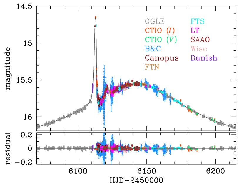
Figure 1.— Lightcurve of OGLE-2012-BLG-0406 showing our best-fit binary-lens model including parallax and orbital motion. The legend on the right of the figure lists the contributing telescopes. All data were taken in the $I$-band, except where otherwise indicated.

3. Modeling

Figure 1 shows the lightcurve of OGLE-2012-BLG-406. The lightcurve displays two main features that deviate significantly from the standard Paczyński curve. The first feature, which peaked at HJD $\sim$ 2456112 (3^rd of July), is produced by the source trajectory grazing the cusp of a caustic. The brightness then quickly drops as the source moves away from the cusp (Schneider & Weiss, 1992; Zakharov, 1995), increases again for a brief period as it passes close to another cusp at HJD $\sim$ 2456121 (12^th of July), and eventually returns to the standard shape as the source moves further away from the caustic structure. The anomalous behavior, when both features are considered, lasts for a total of $\sim$ 15 days, while the full duration of the event is $\gtrsim$120 days. These are typical lightcurve features expected from lensing phenomena involving planetary lenses.

Table 2Lensing Parameters

parameters	standard	parallax		orbit		orbit+parallax
		$u_{0}>0$	$u_{0}<0$	$u_{0}>0$	$u_{0}<0$	$u_{0}>0$	$u_{0}<0$
$\chi^{2}$/dof	6921.019/6383	6850.358/6381	6677.685/6381	6408.371/6381	6408.255/6381	6357.680/6379	6381.358/6379
$t_{0}$ (HJD’)	6141.63 $\pm$ 0.04	6141.70 $\pm$ 0.05	6141.66 $\pm$ 0.05	6141.24 $\pm$ 0.05	6141.28 $\pm$ 0.04	6141.33 $\pm$ 0.05	6141.19 $\pm$ 0.06
$u_{0}$	0.532 $\pm$ 0.001	0.527 $\pm$ 0.001	-0.520 $\pm$ 0.001	0.500 $\pm$ 0.002	-0.499 $\pm$ 0.002	0.496 $\pm$ 0.002	-0.497 $\pm$ 0.002
$t_{\rm E}$ (days)	62.37 $\pm$ 0.06	63.75 $\pm$ 0.18	69.39 $\pm$ 0.32	65.33 $\pm$ 0.20	65.53 $\pm$ 0.15	64.77 $\pm$ 0.19	61.91 $\pm$ 0.42
$s$	1.346 $\pm$ 0.001	1.345 $\pm$ 0.001	1.341 $\pm$ 0.001	1.300 $\pm$ 0.002	1.301 $\pm$ 0.001	1.301 $\pm$ 0.002	1.296 $\pm$ 0.002
$q$ ($10^{-3}$)	5.33 $\pm$ 0.04	5.07 $\pm$ 0.03	4.45 $\pm$ 0.04	6.97 $\pm$ 0.27	6.63 $\pm$ 0.05	5.92 $\pm$ 0.11	6.82 $\pm$ 0.19
$\alpha$	0.852 $\pm$ 0.001	0.864 $\pm$ 0.002	-0.906 $\pm$ 0.002	0.861 $\pm$ 0.002	-0.859 $\pm$ 0.001	0.837 $\pm$ 0.002	-0.810 $\pm$ 0.005
$\rho_{\ast}$ ($10^{-2}$)	1.103 $\pm$ 0.008	1.053 $\pm$ 0.007	0.968 $\pm$ 0.009	1.233 $\pm$ 0.031	1.194 $\pm$ 0.011	1.111 $\pm$ 0.014	1.207 $\pm$ 0.023
$\pi_{{\rm E},N}$	–	0.118 $\pm$ 0.011	-0.414 $\pm$ 0.016	–	–	-0.143 $\pm$ 0.018	0.358 $\pm$ 0.042
$\pi_{{\rm E},E}$	–	-0.033 $\pm$ 0.007	-0.069 $\pm$ 0.009	–	–	0.047 $\pm$ 0.007	0.008 $\pm$ 0.006
$ds/dt$ (yr-1)	–	–	–	0.765 $\pm$ 0.046	0.727 $\pm$ 0.017	0.669 $\pm$ 0.028	0.802 $\pm$ 0.033
$d\alpha/dt$ (yr-1)	–	–	–	1.284 $\pm$ 0.159	-1.108 $\pm$ 0.019	0.497 $\pm$ 0.059	-0.732 $\pm$ 0.085

Note. — HJD’=HJD-2450000.

We begin our analysis by exploring a standard set of solutions that involve modeling the event as a static binary lens. The Paczyński curve representing the evolution of the event for most of its duration is described by three parameters: the time of closest approach between the projected position of the source on the lens plane and the position of the lens photocenter, $t_{0}$, the minimum impact parameter of the source, $u_{0}$, expressed in units of the angular Einstein radius of the lens ($\theta_{\rm E}$), and the duration of time, $t_{\rm E}$ (the Einstein time-scale), required for the source to cross $\theta_{\rm E}$. The binary nature of the lens requires the introduction of three extra parameters: The mass ratio $q$ between the two components of the lens, their projected separation $s$, expressed in units of $\theta_{\rm E}$, and the source trajectory angle $\alpha$ with respect to the axis defined by the two components of the lens. A seventh parameter, $\rho_{\ast}$, representing the source radius normalized by the angular Einstein radius is also required to account for finite-source effects that are important when the source trajectory approaches or crosses a caustic (Ingrosso et al., 2009).

The magnification pattern produced by binary lenses is very sensitive to variations in $s,q$, which are the parameters that affect the shape and orientation of the caustics, and $\alpha$, the source trajectory angle. Even small changes in these parameters can produce extreme changes in magnification as they may result in the trajectory of the source approaching or crossing a caustic (Dong et al., 2006, 2009). On the other hand, changes in the other parameters cause the overall magnification pattern to vary smoothly.

To assess how the magnification pattern depends on the parameters, we start the modeling run by performing a hybrid search in parameter space whereby we explore a grid of $s,q,\alpha$ values and optimize $t_{0},u_{0},t_{\rm E}$ and $\rho_{\ast}$ at each grid point by $\chi^{2}$ minimization using Markov Chain Monte Carlo (MCMC). Our grid limits are set at $-1\leq\log s\leq 1$, $-5\leq\log q\leq 1$, and $0\leq\alpha<2\pi$, which are wide enough to guarantee that all local minima in parameter space have been identified. An initial MCMC run provides a map of the topology of the $\chi^{2}$ surface, which is subsequently further refined by gradually narrowing down the grid parameter search space (Shin et al., 2012a; Street et al., 2013). Once we know the approximate locations of the local minima, we perform a $\chi^{2}$ optimization using all seven parameters at each of those locations in order to determine the refined position of the minimum. From this set of local minima, we identify the location of the global minimum and check for the possible existence of degenerate solutions. We find no other solutions.

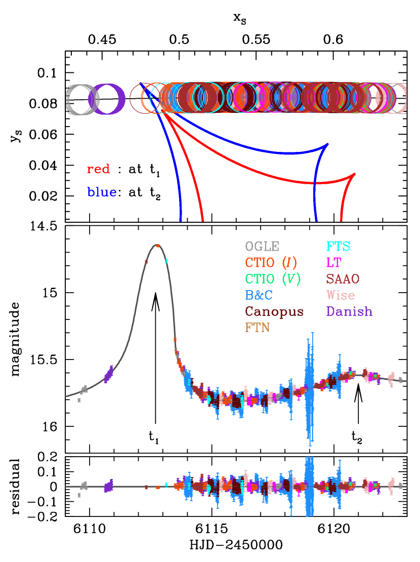
Figure 2.— The bottom panel zooms-in on the anomalous region of the lightcurve presented in Figure 1. At the top panel we display the source trajectory, color coded for the individual contributions of each observatory, and caustic structure at two different times corresponding to the first and second peaks of the anomaly. All scales are normalized by $\theta_{\rm E}$, and the size of the circles corresponds to the size of the source. The first peak deviates the strongest. This is a result of the trajectory of the source grazing the cusp of the caustic at $t_{1}$ (HJD$\sim$2456112), shown in red. The second deviation at $t_{2}$ (HJD$\sim$2456121) is significantly weaker and is due to the source trajectory passing close to another cusp of the caustic, shown in blue. The differences in the shape of the caustic shown at $t_{1}$ and $t_{2}$ are due to the orbital motion of the lens-planet system.

Since our analysis relies on data sets obtained from different telescopes and instruments which use different estimates for the reported photometric precision, we normalize the flux uncertainties of each data set by adjusting them as $e_{i}=f_{i}(\sigma_{0}^{2}+\sigma_{i}^{2})^{1/2}$, where $f_{i}$ is a scale factor, $\sigma_{0}$ are the originally reported uncertainties and $\sigma_{i}$ is an additive uncertainty term for each data set $i$. The rescaling ensures that $\chi^{2}$ per degree of freedom ($\chi^{2}$/dof) for each data set relative to the model becomes unity. Data points with very large uncertainties and obvious outliers are also removed in the process.

In computing finite-source magnifications, we take into account the limb-darkening of the source by modeling the surface brightness as $S_{\lambda}(\vartheta)\propto 1-\Gamma_{\lambda}(1-1.5\cos\vartheta)$ (Albrow et al., 2001), where $\vartheta$ is the angle between the line of sight toward the source star and the normal to the source surface, and $\Gamma_{\lambda}$ is the limb-darkening coefficient in passband $\lambda$. We adopt $\Gamma_{V}=0.74$ and $\Gamma_{I}=0.53$ from the Claret (2000) tables. These values are based on our classification of the stellar type of the source, as subsequently described.

The residuals contained additional smooth structure that the static binary model did not account for. This indicated the need to consider additional second-order effects. The event lasted for $\gtrsim 120$ days, so the positional change of the observer caused by the orbital motion of the Earth around the Sun may have affected the lensing magnification. This introduces subtle long-term perturbations in the event lightcurve by causing the apparent lens-source motion to deviate from a rectilinear trajectory (Gould, 1992; Alcock et al., 1995). Modeling this parallax effect requires the introduction of two extra parameters, $\pi_{{\rm E},N}$ and $\pi_{{\rm E},E}$, representing the components of the parallax vector $\mbox{\boldmath$\pi$}_{\rm E}$ projected on the sky along the north and east equatorial axes respectively. When parallax effects are included in the model, we use the geocentric formalism of Gould et al. (2004) which ensures that the parameters $t_{0}$, $u_{0}$ and $t_{\rm E}$ will be almost the same as when the event is fitted without parallax.

An additional effect that needs to be considered is the orbital motion of the lens system. The lens orbital motion causes the shape of the caustics to vary with time. To a first order approximation, the orbital effect can be modeled by introducing two extra parameters that represent the rate of change of the normalized separation between the two lensing components $ds/dt$ and the rate of change of the source trajectory angle relative to the caustics $d\alpha/dt$ (Albrow et al., 2000).

We conduct further modeling considering each of the higher-order effects separately and also model their combined effect. Furthermore, for each run considering a higher-order effect, we test models with $u_{0}>0$ and $u_{0}<0$ that form a pair of degenerate solutions resulting from the mirror-image symmetry of the source trajectory with respect to the binary-lens axis. For each model, we repeat our calculations starting from different initial positions in parameter space to verify that the fits converge to our previous solution and that there are no other possible minima.

Table 2 lists the optimized parameters for the models we considered. We find that higher-order effects contribute strongly to the shape of the lightcurve. The model including the parallax effect provides a better fit than the standard model by $\Delta\chi^{2}=243.3$. The orbital effect also improves the fit by $\Delta\chi^{2}=512.8$. The combination of both parallax and orbital effects improves the fit by $\Delta\chi^{2}=563.3$. Due to the $u_{0}>0$ and $u_{0}<0$ degeneracy, there are two solutions for the orbital motion + parallax model which have similar $\chi^{2}$ values. Models involving the xallarap effect (source orbital motion) were also considered but they did not outperform equivalent models involving only parallax.

In Figure 1, we present the best-fit model lightcurve superposed on the observed data. Figure 2 displays an enlarged view of the perturbation region of the lightcurve along with the source trajectory with respect to the caustic. The follow-up observations cover critical features of the perturbation regions that were not covered by the survey data. We note that the caustic varies with time and thus we present the shape of the caustic at the times of the first ($t_{1}$=HJD$\sim$2456112) and second perturbations ($t_{2}$=HJD$\sim$2456121). The source trajectory grazes the caustic structure at $t_{1}$ causing a substantial increase in magnification. As the caustic structure and trajectory evolve with time, the trajectory approaches another cusp at $t_{2}$, but does not cross it. This second approach causes an increase in magnification which is appreciably lower than that of the first encounter at $t_{1}$. The source trajectory is curved due to the combination of the parallax and orbital effects.

The mass and distance to the lens are determined by

$$M_{\rm tot}={\theta_{\rm E}\over\kappa\pi_{\rm E}};\qquad D_{\rm L}={{\rm AU}\over\pi_{\rm E}\theta_{\rm E}+\pi_{\rm S}},$$ (1)

where $\kappa=4G/(c^{2}{\rm AU})$ and $\pi_{\rm S}$ is the parallax of the source star (Gould, 1992). To determine these physical quantities we require the values of $\pi_{\rm E}$ and $\theta_{\rm E}$. Modeling the event returns the value of $\pi_{\rm E}$, whereas $\theta_{\rm E}=\theta_{\ast}/\rho_{\ast}$ depends on the angular radius of the source star, $\theta_{\ast}$, and the normalized source radius, $\rho_{\ast}$, which is also returned from modeling (see Table 2). Therefore, determining $\theta_{\rm E}$ requires an estimate of $\theta_{\ast}$.

To estimate the angular source radius, we use the standard method described in Yoo et al. (2004). In this procedure we first measure the dereddened color and brightness of the source star by using the centroid of the giant clump as a reference because its dereddened magnitude $I_{0,c}=14.45$ (Nataf et al., 2013) and color $(V-I)_{0,c}=1.06$ (Bensby et al., 2011) are already known. For this calibration, we use a color-magnitude diagram obtained from CTIO observations in the $I$ and $V$ bands. We then convert the $V-I$ source color to $V-K$ using the color-color relations from Bessell and Brett (1988) and the source radius is obtained from the $\theta_{\ast}$-$(V-K)$ relations of Kervella et al. (2004). We derive the dereddened magnitude and color of the source star as $I_{0}=14.62$ and $(V-I)_{0}=1.12$ respectively. This confirms that the source star is an early K-type giant. The estimated angular source radius is $\theta_{\ast}=5.94\pm 0.51$ $\mu$as. Combining this with our evaluation of $\rho_{\ast}$, we obtain $\theta_{\rm E}=0.53\pm 0.05$ mas for the angular Einstein radius of the lens.

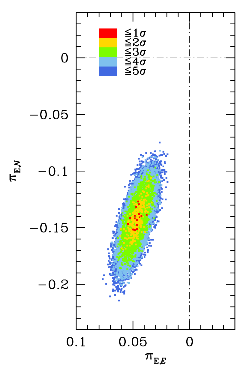
Figure 3.— $\Delta\chi^{2}$ contours for the parallax parameters derived from our MCMC fits for the best binary-lens model including orbital motion and the parallax effect.

Our analysis is consistent with the results of Poleski et al. (2013). We confirm that the lens is a planetary system composed of a giant planet orbiting a low-mass star and we report the refined parameters of the system. Poleski et al. (2013) reported that there existed a pair of degenerate solutions with $u_{0}>0$ and $u_{0}<0$, although the positive $u_{0}$ solution is slightly preferred with $\Delta\chi^{2}=13.6$. We find a consistent result that the positive $u_{0}$ solution is preferred but the degeneracy is better discriminated by $\Delta\chi^{2}=23.7$.

The error contours of the parallax parameters for the best-fit model are presented in Figure 3. The uncertainty of each parameter is determined from the distribution of MCMC chain, and the reported uncertainty corresponds to the standard deviation of the distribution. We list the physical parameters of the system in Table 3 and their posterior probability distributions are shown in Figure 4.

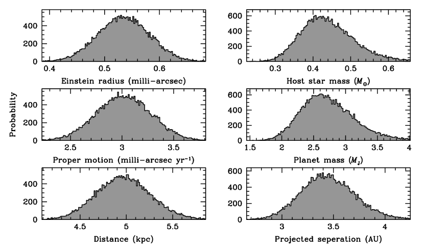
Figure 4.— The physical parameter uncertainties pertaining to the lens as derived from the MCMC runs optimizing our binary-lens model including parallax and orbital motion for the $u_{0}>0$ trajectory.

The lens lies $D_{\rm L}=4.97\pm 0.29$ kpc away in the direction of the Galactic Bulge. The more massive component of the lens has mass $M_{\star}=0.44\pm 0.07$ $M_{\odot}$ so it is an early M-type dwarf star and its companion is a super-Jupiter planet with a mass $M_{\rm p}=2.73\pm 0.43$ $M_{\rm J}$. The projected separation between the two components of the lens is $d_{\perp}=3.45\pm 0.26$ AU. The geocentric relative proper motion between the lens and the source is $\mu_{\rm Geo}=\theta_{\rm E}/t_{\rm E}=3.02\pm 0.26$ milli-arcsec yr^-1. In the Heliocentric frame, the proper motion is $\mbox{\boldmath$\mu$}_{\rm Helio}=(\mu_{N},\mu_{E})=(-2.91\pm 0.26,1.31\pm 0.16)$ milli-arcsec yr^-1.

Table 3Physical Parameters

parameters	quantity
Mass of the host star ($M_{\star}$)	0.44 $\pm$ 0.07 $M_{\odot}$
Mass of the planet ($M_{\rm p}$)	2.73 $\pm$ 0.43 $M_{\rm J}$
Distance to the lens ($D_{\rm L}$)	4.97 $\pm$ 0.29 kpc
Projected star-planet separation ($d_{\perp}$)	3.45 $\pm$ 0.26 AU
Einstein radius ($\theta_{\rm E}$)	0.53 $\pm$ 0.05 milli-arcsec
Geocentric proper motion ($\mu_{\rm Geo}$)	3.02 $\pm$ 0.26 milli-arcsec yr-1

We note that the derived physical lens parameters are somewhat different from those of Poleski et al. (2013). Specifically, the mass of the host star derived in Poleski et al. (2013) is 0.59 $M_{\odot}$, which is $\sim$ 34% greater than our estimate. Half of this difference comes from the slightly larger Einstein radius obtained by Poleski et al. (2013) from the OGLE-IV photometry and the remaining part from the slightly larger $\pi_{{\rm E},N}$ component of the parallax obtained from modeling the survey and follow-up photometry as presented in this paper. It should be noted that the parameters derived by both our and thePoleski et al. (2013) models are consistent within the 1-$\sigma$ level.

To further check the consistency between our model and that of Poleski et al. (2013), we conducted additional modeling based on different combinations of data sets. We first test a model based on OGLE data exclusively in order to see whether we can retrieve the physical parameters reported in Poleski et al. (2013). From this modeling, we derive physical parameters consistent with those of Poleski et al. (2013), indicating that the differences are due to the additional coverage provided by the follow-up observations. We conducted another modeling run using OGLE observations but also included CTIO, FTS and SAAO data, i.e. those datasets covering the anomalous peak. This modeling run resulted in physical parameters that are consistent with the values extracted from fitting all combined data together, as reported in this paper. This indicates that the differences between Poleski et al. (2013) and this analysis, although consistent within the 1-$\sigma$ level, come mainly from follow-up data that provide better coverage of the perturbation. Therefore, using survey and follow-up data together, we arrive at a more accurate determination of the $\rho$ and $\pi_{{\rm E},N}$ parameters, which leads to a refinement of the physical parameters of the planetary system.

4. Conclusions

Microlensing event OGLE-2012-BLG-0406 was intensively observed by survey and follow-up groups using 10 different telescopes around the world. Anomalous deviations observed in the lightcurve were recognized to be due to the presence of a planetary companion even before the event reached its central peak. The anomalous behavior was first identified and assessed automatically via software agents. Most follow-up teams responded to these alerts by adjusting their observing strategies accordingly. This highlights the importance of circulating early models to the astronomical community that help to identify important targets for follow-up observations (Shin et al., 2012b). There are $\sim$100 follow-up alerts circulated annually, $\sim$10% of which turn out to be planet candidates.

Our analysis of the combined data is consistent with the results of Poleski et al. (2013) and we report the refined parameters of the system. We find that this refinement is mainly due to follow-up observations over the anomaly. The primary lens with mass $M_{\star}=0.44\pm 0.07$ $M_{\odot}$ is orbited by a planetary companion with mass $M_{\rm p}=2.73\pm 0.43$ $M_{\rm J}$ at a projected separation of $d_{\perp}=3.45\pm 0.26$ AU. The distance to the system is $D_{\rm L}=4.97\pm 0.29$ kpc in the direction of the Galactic Bulge.

This is the fourth cold super-Jupiter planet around a low-mass star discovered by microlensing (Dong et al., 2009; Batista et al., 2011; Yee et al., 2012) and the first such system whose characteristics were derived solely from microlensing data, without considering any external information.

Microlensing is currently the only way to obtain high precision mass measurements for this type of system. Radial velocity, in addition to the ${m\sin{\rm i}}$ degeneracy, at present does not have long enough data streams to measure the parameters of such systems. However, recently Montet et al. (2013) have developed a promising new method to discover them using a combination of radial velocity and direct imaging. They identify long term trends in radial velocity data and use adaptive optics imaging to rule out the possibility that these are due to stars. This means that the trends are either due to large planets or brown dwarfs. This approach does not yield precise characterization but provides important statistical information. Their results are consistent with gravitational microlensing estimates of planet abundance in that region of parameter space.

The precise mechanism of how such large planets form and evolve around low mass stars is still an open question. Radial velocity and transit surveys have been finding massive gas-giant planets around FGK-stars for years (Batalha et al., 2013) but these stars have protoplanetary disks that are sufficiently massive to allow the formation of super-Jupiter planets. On the other hand, protoplanetary disks around M-dwarfs have masses of only a few Jupiter mass so massive gas giants should be relatively hard to produce (Apai, 2013).

Recent observational studies have revealed that protoplanetary disks are as common around low mass stars as higher-mass stars (Williams & Cieza, 2011), arguing for the same formation processes. In addition, there is mounting evidence, but not yet conclusive, that disks last much longer around low-mass stars (Apai, 2013). Longer disk lifetimes may be conducive to the formation of super-Jupiters. The microlensing discoveries suggest that giant planets around low-mass stars may be as common as around higher-mass stars but may not undergo significant migration (Gould et al., 2010).

Simulations using the core accretion formalism can produce such planets within reasonable disk lifetimes of a few Myr (Mordasini et al., 2012) provided the core mass is sufficiently large or the opacity of the planet envelope during gas accretion is decreased by assuming that the dust grains have grown to larger sizes than the typical interstellar values (R. Nelson, private communication). Furthermore, gravitational instability models of planet formation can also potentially produce such objects when the opacity of the protoplanetary disk is low enough to allow local fragmentation at greater distances from the host star, and subsequently migrating the planet to distances of a few AU.

It is worth noting that highly magnified microlensing events involving extended stellar sources may produce appreciable polarization signals (Ingrosso et al., 2012). If such signals are observed during a microlensing event, they can be combined with photometric observations to place further constraints on the lensing geometry and physical properties of the lens.

References

- Alard and Lupton (1998) Alard, C. & Lupton, R. H. 1998, ApJ, 503, 325
- Albrow et al. (2001) Albrow, M. D., An, J., Beaulieu, J.-P., et al. 2001, ApJ, 549, 759
- Albrow et al. (2000) Albrow, M. D., Beaulieu, J.-P., Caldwell, J. A. R., et al. 2000, ApJ, 534, 894
- Albrow et al. (2009) Albrow, M. D., Horne, K., Bramich, D. M., et al. 2009, MNRAS, 397, 2099
- Alcock et al. (1995) Alcock, C., Allsman, R. A., Alves, D., et al. 1995, ApJ, 454, 125
- Apai (2013) Apai, D., 2013, Astronomische Nachrichten, 334, 57
- Batalha et al. (2013) Batalha, N. M., Rowe, J. F., Bryson, S. T., et al. 2013, ApJS, 204, 24
- Batista et al. (2011) Batista, V., Gould, A., Dieters, S., et al. 2011, A&A, 529, 102
- Beaulieu et al. (2006) Beaulieu, J.-P., Bennett, D. P., Fouqué, P., et al. 2006, Nature, 439, 437
- Bensby et al. (2011) Bensby, T., Adén, D., Meléndez, J., et al. 2011, A&A, 533, A134
- Bessell and Brett (1988) Bessell, M. S. & Brett, J. M. 1988, PASP, 100, 1134
- Bond et al. (2001) Bond, I. A., Abe, F., Dodd, R. J., et al. 2001, MNRAS, 327, 868
- Bozza (2010) Bozza, V. 2010, MNRAS, 408, 2188
- Bramich (2008) Bramich, D. M. 2008, MNRAS, 386, L77
- Cassan et al. (2012) Cassan, A., Kubas, D., Beaulieu, J.-P., et al. 2012, Nature, 481, 167
- Claret (2000) Claret, A. 2000, A&A, 363, 1081
- Kim et al. (2009) Kim, D., & Han, C., & Park, B.-J. 2009, JKAS, 42, 39
- Dominik (2010) Dominik, M. 2010, Generay Relativity and Gravitation, 42, 9
- Dominik et al. (2008) Dominik, M., Horne, K., Allan, A., et al. 2008, Astronomische Nachrichten, 329, 248
- Dominik (2010) Dominik, M., Jørgensen, U. G., Rattenbury, N. J., et al. 2010, Astronomische Nachrichten, 331, 671
- Dominik et al. (2007) Dominik, M., Rattenbury, N.J., Allan, A., et al. 2007, MNRAS, 380, 792
- Dong et al. (2009) Dong, S., Bond, I. A., Gould, A., et al. 2009, ApJ, 698, 1826
- Dong et al. (2006) Dong, S., DePoy, D. L., Gaudi, B. S., et al. 2006, ApJ, 642, 842
- Dong et al. (2009) Dong, S., Gould, A., Udalski, A., et al. 2009, ApJ, 695, 970
- Gaudi (2011) Gaudi, B. S. 2011, Exoplanets (book), 79
- Gaudi (2012) Gaudi, B. S. 2012, ARA&A, 50, 411
- Gaudi et al. (2008) Gaudi, B. S., Bennett, D. P., Udalski, A., et al. 2008, Science, 319, 927
- Gould (1992) Gould, A. 1992, ApJ, 392, 442
- Gould et al. (2004) Gould, A. 2004, ApJ, 606, 319
- Gould et al. (2006) Gould, A., Udalski, A., An, D., et al. 2006, ApJ, 644, L37
- Gould et al. (2010) Gould, A., Dong, S., Gaudi, B. S., et al 2010, ApJ, 720, 1073
- Griest and Safizadeh (1998) Griest, K., & Safizadeh, N. 1998, ApJ, 500, 37
- Han et al. (2013) Han, C., Udalski, A., Choi, J.-Y., et al. 2013, ApJ, 762, 28
- Horne et al. (2009) Horne, K., Snodgrass, C., Tsapras, Y., 2009, MNRAS, 396, 2087
- Ingrosso et al. (2012) Ingrosso, G., Novati, S. Calchi, de Paolis, F., et al. 2012, MNRAS, 426, 1496
- Ingrosso et al. (2009) Ingrosso, G., Novati, S. Calchi, de Paolis, F., et al. 2009, MNRAS, 399, 219
- Johnson et al. (2010) Johnson, J. A., Howard, A. W., Marcy, G. W., et al. 2010, PASP, 122, 149
- Kains et al. (2013) Kains, N., Street, R. A., Choi, J.-Y., et al. 2013, A&A, 552, 70
- Kalas et al. (2005) Kalas, P. Graham, J. R., Clampin, M. 2005, Nature, 435, 1067
- Kervella et al. (2004) Kervella, P., Bersier, D. Mourard, D. et al. 2004, A&A, 428, 587
- Laughlin et al. (2004) Laughlin, G., Bodenheimer, P., Adams, F. C. 2004, ApJ, 612, 73
- Lecar et al. (2006) Lecar, M., Podolak, M., Sasselov, D., Chiang, E. 2006, ApJ, 640, 1115
- Mao and Paczyński (1991) Mao, S., & Paczyński, B. 1991, ApJ, 374, L37
- Miguel et al. (2011) Miguel, Y., Guilera, O. M., Brunini, A., 2011, MNRAS, 417, 314
- Montet et al. (2013) Montet, B. T., Crepp, J. R., Johnson, J. A., et al. 2013, ApJ, submitted
- Mordasini et al. (2012) Mordasini, C., Alibert, Y., Benz, W., et al. 2012, A&A, 547, 112
- Nataf et al. (2013) Nataf, D. M., Gould, A., Fouqué, P., et al. 2013, ApJ, 769, 88
- Paczyński (1986) Paczyński, B. 1986, ApJ, 304, 1
- Poleski et al. (2013) Poleski, R., Udalski, A., Dong, S., et al. 2013, ApJ, submitted
- Schneider & Weiss (1992) Schneider, P. & Weiss, A. 1992, A&A, 260, 1
- Shin et al. (2012a) Shin, I.-G., Choi, J.-Y., Park, S.-Y., et al. 2012, ApJ, 746, 127
- Shin et al. (2012b) Shin, I.-G., Han, C., Gould, A., et al. 2012, ApJ, 760, 116
- Street et al. (2013) Street, R., Choi, J.-Y., Tsapras, Y., et al. 2013, ApJ, 763, 67
- Sumi et al. (2003) Sumi, T., Abe, F., Bond, I. A., et al. 2003, ApJ, 591, 204
- Sumi et al. (2010) Sumi, T., Bennett, D. P., Bond, I. A., et al. 2010, ApJ, 710, 1641
- Sumi et al. (2011) Sumi, T., Kamiya, K., Bennett, D. P., et al. 2011, Nature, 473, 349
- Tsapras et al. (2003) Tsapras, Y., Horne, K., Kane, S., et al. 2003, MNRAS, 343, 1131
- Tsapras et al. (2009) Tsapras, Y., Street, R., Horne, K., et al. 2009, Astronomische Nachrichten, 330, 4
- Udalski (2003) Udalski, A. 2003, Acta Astron., 53, 291
- Williams & Cieza (2011) Williams, P. W., Cieza, A. L., 2011, ARA&A, 49, 67
- Yee et al. (2012) Yee, J., Shvartzvald, Y., Gal-Yam, A., et al. 2012, ApJ, 775, 102
- Yoo et al. (2004) Yoo, J., DePoy, D. L., Gal-Yam, A., et al. 2004, ApJ, 603, 139
- Zakharov (1995) Zakharov, A. F. 1995, A&A, 293, 1