Towards understanding thermal jet quenching via lattice simulations

Abstract:

After reviewing how simulations employing classical lattice gauge theory permit to test a conjectured Euclideanization property of a light-cone Wilson loop in a thermal non-Abelian plasma, we show how Euclidean data can in turn be used to estimate the transverse collision kernel, $C(k_{\perp})$, characterizing the broadening of a high-energy jet. First results, based on data produced recently by Panero et al, suggest that $C(k_{\perp})$ is enhanced over the known NLO result in a soft regime $k_{\perp}<$ a few $T$. The shape of $k_{\perp}^{3}C(k_{\perp})$ is consistent with a Gaussian at small $k_{\perp}$.

1 Motivation

Among the main observables measured in heavy ion collision experiments are “hard probes”, i.e. particle-like objects having an energy much larger than the temperature. Hard probes can either be colour-neutral, such as photons, or coloured, such as jets. In the case of photons, the probe escapes the thermal medium unaltered, and its average production rate reflects directly the physics of the production mechanism. In the case of jets, in contrast, the probe experiences a complicated evolution, with the jet losing its virtuality to radiation, its energy and longitudinal momentum to radiation and collisions with the medium, but simultaneously gaining transverse momentum from collisions, leading to broadening. These phenomena may collectively be referred to as jet quenching; for reviews, see e.g. refs. [1]–[7].

One quantity characterizing many of the mentioned processes is the so-called transverse collision kernel, denoted by $C(k_{\perp})$. Its appearance in the context of jet broadening is sketched in sec. 2, whereas a recent discussion of its role in photon production can be found in ref. [8]. The focus of the present study is a non-perturbative estimate of $C(k_{\perp})$ with the help of lattice gauge theory, following ideas put forward by Caron-Huot in the context of an NLO computation [9].

2 Momentum broadening and the light-cone Wilson Loop

Let $P(k_{\perp},L)$ be a probability distribution, normalized as $\int\frac{{\rm d}^{2}{\bf k}_{\perp}}{(2\pi)^{2}}P(k_{\perp},L)=1$, of transverse momenta of a jet, once it has traversed a path of length $L\gg 1/\pi T$ within a medium of temperature $T$. The classical nature of $P$ could originate from decoherence due to many collisions. Energy and longitudinal momenta are assumed hard, $k_{0},k_{\parallel}\gg\pi T$, with $\pi T$ denoting a typical energy scale of a relativistic plasma, but virtuality is small and will be neglected in the following.

Considering a jet seeded by a quark, $P(k_{\perp},L)$ is given by a Fourier transform of a light-cone Wilson loop in the fundamental representation (our discussion follows appendix D of ref. [6]):

$$P(x_{\perp},L)\;=\;\frac{1}{N_{\rm c}}{\rm Tr\,}\langle\mathcal{W}_{\mbox{\tiny\rm{F}}}(x_{\perp},L,t)\rangle\;,\quad P(k_{\perp},L)\;=\;\int\!{\rm d}^{2}{\bf x}_{\perp}\,e^{-i{\bf k}_{\perp}\cdot{\bf x}_{\perp}}\,P(x_{\perp},L)\;,$$ (1)

where $t$ denotes time. Along the light-cone, $t=L$, so normally one argument is suppressed. In the case of a jet seeded by a gluon, the Wilson loop is in the adjoint representation. $P(x_{\perp},L)$ evolves as

$$\frac{{\rm d}P(x_{\perp},L)}{{\rm d}L}=-V(x_{\perp})\,P(x_{\perp},L)\;,$$ (2)

where $V(x_{\perp})$ may be called a dipole cross section (we refer to it as a transverse potential). The transverse collision kernel, $C(k_{\perp})$, contains the same information as $V(x_{\perp})$ but in Fourier space:

$$V(x_{\perp})=\int\!\frac{{\rm d}^{2}{\bf k}_{\perp}}{(2\pi)^{2}}\Bigl{(}1-e^{i{\bf k}_{\perp}\cdot{\bf x}_{\perp}}\Bigr{)}\,C(k_{\perp})\;.$$ (3)

Consequently, the probability distribution of the transverse momenta obeys

$$\frac{{\rm d}P(k_{\perp},L)}{{\rm d}L}=\int\!\frac{{\rm d}^{2}{\bf q}_{\perp}}{(2\pi)^{2}}\;C(q_{\perp})\;[P(k_{\perp}-q_{\perp},L)-P(k_{\perp},L)]\;.$$ (4)

In the following we refer to the extent of the Wilson loop by $t$ rather than $L$.

The goal is thus to extract the damping rate of a real-time Wilson loop, eq. (2). A direct determination with Euclidean lattice QCD is probably beyond reach because two analytic continuations are needed [10]. On the other hand it has been argued [9] that for $k_{\perp}\ll\pi T$ the dominant contribution to the collision kernel resides in soft thermal modes, which are not sensitive to the velocity of the seeding parton. A possible strategy is to tilt the seeding parton beyond the light cone into the space-like domain upon which the associated Wilson loop becomes amenable to Euclidean methods. As a first step, we test this argument by making use of classical lattice gauge theory, which correctly represents the physics of the soft gauge fields [11, 12]. A great advantage is that classical simulations are carried out directly in real time, avoiding any analytic continuation.

3 Classical lattice gauge theory

The Hamiltonian formalism [13] of classical lattice gauge theory is naturally formulated in a fixed temporal gauge $A^{0}=0$. Then its degrees of freedom, colour-electric fields $E_{j}=E^{a}_{j}T^{a}\in$ su(3) and spatial links $U_{j}\in$ SU(3), live on three-dimensional time slices. The theory is parametrized by a single dimensionless number $\beta_{\mbox{\tiny\rm{G}}}\equiv 2N_{\rm c}/(g^{2}Ta)$ with $N_{\rm c}$ the number of colours, $g^{2}\equiv 4\pi\alpha_{s}$ a renormalized gauge coupling, and $a$ the lattice spacing, respectively. The Hamiltonian reads

$$H_{\mbox{\scriptsize cl}}=\sum_{\bf x}\Big{\{}\sum_{i=1}^{3}{\rm Tr\,}[E_{i}^{2}({\bf x})]+\frac{1}{2N_{\rm c}}\sum_{i,j=1}^{3}{\rm Tr\,}[1-P_{ij}({\bf x})]\Big{\}}\;,$$ (5)

where $P_{ij}$ denotes a plaquette in the $(i,j)$-plane. The associated local Gauss constraint $G({\bf x})=\sum_{i}[E_{i}({\bf x})-U^{\dagger}_{i}({\bf x}-\hat{i})E_{i}({\bf x}-\hat{i})U_{i}({\bf x}-\hat{i})]$ singles out the physically admissible $G({\bf x})=0$ configurations. The classical equations of motion read

$$a\partial_{t}U_{j}({\bf x},t)=i(2N_{\rm c})^{\frac{1}{2}}E_{j}({\bf x},t)U_{j}({\bf x},t)\;,$$ (6)

$$a\partial_{t}E_{i}^{b}({\bf x},t)=-\Big{(}\frac{2}{N_{\rm c}}\Big{)}^{\frac{1}{2}}{\mathop{\mbox{Im}}{\rm Tr\,}}\Big{[}T^{b}U_{i}({\bf x},t)\sum_{|j|\neq i}S^{\dagger}_{ij}({\bf x},t)\Big{]}\;,$$ (7)

where $S_{ij}$ denotes the staple in a $(i,j)$-plane which closes to a plaquette when multiplied by $U_{i}^{\dagger}$.

Initial conditions are generated with the weight $P[U,E]\propto e^{-\beta_{\mbox{\tiny\rm{G}}}H_{\mbox{\scriptsize cl}}}\Pi_{\bf x}\delta(G({\bf x}))$, by making use of an algorithm described in ref. [14]. Subsequently $U$ and $E$ are evolved in a forward Euler leap-frog scheme with temporal lattice spacing $a_{t}=a/100$, based on eqs. (6), (7). At each integer step in time $t=na/v$ a copy of the gauge links is saved and a light-cone Wilson line is constructed by appropriate averages of links above and below the actual path as shown in fig. 1(left). Monitoring the large-time behaviour of the Wilson loop, a transverse potential is subsequently extracted from the exponential damping as in eq. (2) (now with $L\to t$),

$$V(x_{\perp})\equiv-\lim_{t\to\infty}\frac{\partial_{t}P(x_{\perp},t)}{P(x_{\perp},t)}\;.$$ (8)

The potential here is a function of $x_{\perp}$ as well as the velocity $v$, as illustrated in fig. 1(left). (In ref. [10] the same object was denoted by $-\mathop{\mbox{Im}}V$, motivated by the time evolution $\sim e^{-iEt}$.)

Figure 1: Left: A tilted lattice Wilson loop in Minkowskian spacetime. Right: The transverse potential in the adjoint representation (darker symbols) for different velocities at $\beta_{\mbox{\tiny\rm{G}}}=64$ and $N/\beta_{\mbox{\tiny\rm{G}}}=1.22$, scaled by $4/9$. The results for the fundamental Wilson loop [10] at $N/\beta_{\mbox{\tiny\rm{G}}}=1.5$ are given with the lighter symbols.

As an example of results that can be obtained, the transverse potential extracted from simulations with $\beta_{\mbox{\tiny\rm{G}}}=64$ on a $N^{3}=78^{3}$ (adjoint rep., scaled with $C_{\mbox{\tiny\rm{F}}}/C_{\mbox{\tiny\rm{A}}}=4/9$) and $N^{3}=96^{3}$ (fundamental rep.) lattice is shown in fig. 1(right) as a function of $x_{\perp}$. For extracting the damping rate from eq. (8), a fitting range is needed that allows for a compromise between signal strength on one hand and an asymptotic exponential behavior of the Wilson loop on the other. Once a range is chosen, a single exponential fit is deployed to measure the value of $V(x_{\perp})$, with systematic errors estimated from the variation of the results when moving the fitting range to later times.

A central argument in the analysis of ref. [9] is that the contribution to the thermal light-cone Wilson loop from soft (colour-electric and colour-magnetic) gauge fields should not be sensitive to crossing the light cone. This argument can be tested through our simulations: results for several $v$ are plotted in fig. 1(right). Quantitative changes are observed as $v$ increases, but there does not appear to be any qualitative transition in the dynamics for $v>1$.

To summarize, classical lattice gauge theory simulations support the theoretical arguments given in ref. [9] and give direct physical insight of the behaviour of relevant observables in Minkowskian spacetime, without complications related to analytic continuation. For quantitative results, however, the Euclidean results of ref. [15] are to be used, because within classical lattice gauge theory the Debye mass parameter cannot be tuned to a physical regularization independent value; it rather changes rapidly with the lattice spacing.

4 How to extract the transverse collision kernel

Suppose now that $V(x_{\perp})$ has been computed non-perturbatively at distances $x_{\perp}\mathop{\raise 1.29167pt\hbox{$>$\kern-7.5pt\raise-4.73611pt\hbox{$\sim$}}}1/(gT)$ with simulations like those in ref. [15] and that a continuum limit has been taken. We may then try to invert the relation between the potential and the transverse collision kernel, eq. (3), in order to estimate $C(k_{\perp})$ in the infrared domain $k_{\perp}\mathop{\raise 1.29167pt\hbox{$<$\kern-7.5pt\raise-4.73611pt\hbox{$\sim$}}}gT$, in which perturbation theory is slowly convergent [9] (for $k_{\perp}\mathop{\raise 1.29167pt\hbox{$<$\kern-7.5pt\raise-4.73611pt\hbox{$\sim$}}}g^{2}T/\pi$ the problem becomes genuinely non-perturbative [16]). We start by showing how the inversion can be carried out in principle.

In the presence of an ultraviolet regularization, such as a lattice cutoff, the first factor on the right-hand side of eq. (3) normalizes the potential to zero at vanishing distance. Omitting this overall normalization for the moment (it will be imposed in a different fashion in a moment), eq. (3) can formally be inverted through a Fourier transform:

$$C(k_{\perp})=-\int\!{\rm d}^{2}{\bf x}_{\perp}\,e^{-i{\bf k}_{\perp}\cdot{\bf x}_{\perp}}V(x_{\perp})=-2\pi\int_{0}^{\infty}\!{\rm d}x_{\perp}\,x_{\perp}\,J_{0}(k_{\perp}x_{\perp})\,V(x_{\perp})\;,$$ (9)

where the angular integral was carried out, and $J_{0}$ is a Bessel function. The asymptotics of $J_{0}$,

$$J_{0}(k_{\perp}x_{\perp})\;\stackrel{{\scriptstyle k_{\perp}x_{\perp}\gg 1}}{{\approx}}\;\sqrt{\frac{2}{\pi k_{\perp}x_{\perp}}}\,\cos\Bigl{(}k_{\perp}x_{\perp}-\frac{\pi}{4}\Bigr{)}\;,$$ (10)

implies however that the integral is typically not absolutely convergent at large $x_{\perp}$. For example, the non-perturbative asymptotics originating from three-dimensional pure Yang-Mills theory obeys the string-theory predicted asymptotics [17]

$$V(x_{\perp})\;\stackrel{{\scriptstyle g^{2}Tx_{\perp}\gg 1}}{{\approx}}\;\sigma x_{\perp}+\mu+\frac{\gamma}{x_{\perp}}\;.$$ (11)

All of these terms decay too slowly for eq. (9) to be absolutely integrable. (The coefficient $\mu$ is related to the overall normalization, as alluded to above.)

It is possible, however, to subtract the problematic terms and carry out the inverse transform on a faster decaying remainder. Concretely, making use a dimensionally regularized Fourier transform,

$$\mathcal{F}\biggl{[}\frac{1}{k_{\perp}^{\nu}}\biggr{]}\;\equiv\;\int\!\frac{{\rm d}^{2-2\epsilon}{\bf k}_{\perp}}{(2\pi)^{2-2\epsilon}}\frac{e^{i{\bf k}_{\perp}\cdot{\bf x}_{\perp}}}{k_{\perp}^{\nu}}\;=\;\frac{\Gamma(1-\epsilon-\frac{\nu}{2})}{\Gamma(\frac{\nu}{2})}\frac{1}{2^{\nu}\pi^{1-\epsilon}x_{\perp}^{2-2\epsilon-\nu}}\;,$$ (12)

which implies $\mathcal{F}[1/k_{\perp}]=1/(2\pi x_{\perp})$ as well as $\mathcal{F}[1/k_{\perp}^{3}]=-x_{\perp}/(2\pi)$, and tuning $\sigma,\mu,\gamma$ such that

$$\lim_{x_{\perp}\to\infty}x_{\perp}\biggl{\{}V(x_{\perp})-\biggl{[}\sigma x_{\perp}+\mu+\frac{\gamma}{x_{\perp}}\biggr{]}\biggr{\}}=0\;,$$ (13)

we obtain a subtracted version of the (inverse) Fourier transform:

$$\frac{C(k_{\perp})}{2\pi}\;=\;\frac{\sigma}{k_{\perp}^{3}}-\frac{\gamma}{k_{\perp}}+\int_{0}^{\infty}\!{\rm d}x_{\perp}\,x_{\perp}\,J_{0}(k_{\perp}x_{\perp})\biggl{[}\sigma x_{\perp}+\mu+\frac{\gamma}{x_{\perp}}-V(x_{\perp})\biggr{]}\;,\quad k_{\perp}>0\;.$$ (14)

The integral here is convergent in a confining theory (provided that the potential does not diverge too fast at short distances, which is not the case).

5 A first numerical test

In a practical setting, where $V(x_{\perp})$ contains errors and is only known in a finite interval, it is not clear a priori whether eq. (14) can yield useful results. The reason is that $J_{0}$ is oscillatory, so a kind of sign problem (significance loss) takes place. Nevertheless the problem is less serious at small $k_{\perp}$, precisely the domain of most interest, so it appears worthwhile to carry out a test.

For the test, we make use of the data of ref. [15]. As an example, we consider the so-called “cold” set ($T\approx 400$ MeV) at the lattice couplings $\beta_{\mbox{\tiny\rm{G}}}=14,16,18$; these $\beta_{\mbox{\tiny\rm{G}}}$-values are chosen as a compromise for which data extend both to short and large distances. The central values at distances $r>r_{0}$, where $r_{0}\approx 2.2/g_{\mbox{\tiny\rm{E}}}^{2}$ is the Sommer scale, are used in a $\chi^{2}$-minimization to determine the parameters of eq. (13). (For $\beta_{\mbox{\tiny\rm{G}}}=14$ this corresponds to the 6 largest distances; for $\beta_{\mbox{\tiny\rm{G}}}=16$ to 5; for $\beta_{\mbox{\tiny\rm{G}}}=18$ to 4.) Note that such a fit, at finite distances and $\beta_{\mbox{\tiny\rm{G}}}$ and with the colour-electric “decorations” present in the Wilson loop, does not necessarily reproduce the pure Yang-Mills values [17], for instance we find $\gamma>0$. Having fixed the parameters, eq. (14) is subsequently estimated through

$$\frac{C(k_{\perp})}{2\pi}\;\simeq\;\frac{\sigma}{k_{\perp}^{3}}-\frac{\gamma}{k_{\perp}}+{\frac{1}{2}\,}\sum_{i=1}^{i_{\mbox{\tiny\rm{max}}}}\bigl{[}x_{\perp,i}-x_{\perp,i-1}\bigr{]}\bigl{[}\phi(x_{\perp,i})+\phi(x_{\perp,i-1})\bigr{]}\;,$$ (15)

where $i$ numerates the distances at which data is available, $x_{\perp,0}\equiv 0$, and $\phi$ denotes the integrand:

$$\phi(x_{\perp}) \equiv x_{\perp}\,J_{0}(k_{\perp}x_{\perp})\biggl{[}\sigma x_{\perp}+\mu+\frac{\gamma}{x_{\perp}}-V(x_{\perp})\biggr{]}\;,\quad x_{\perp}>0\;,$$ (16)

$$\phi(0) \equiv \gamma\;.$$ (17)

The definition in eq. (17) originates from $J_{0}(0)=1$ and the observation that $V(x_{\perp})$ diverges more slowly than $1/x_{\perp}$ at short distances. In order to produce an error band, we have generated $\sim 100$ mock configurations with the given central values and errors from ref. [15], treating the errors at various $x_{\perp,i}$ as independent from each other. Equation (15) is evaluated for each configuration, and subsequently the central values and their variances are determined as usual.

   

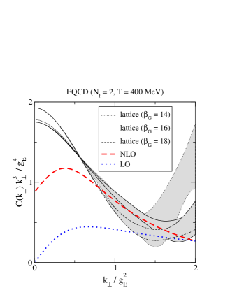
Figure 2: Left: The transverse collision kernel extracted from eq. (15) by making use of lattice data from ref. [15], compared with the NLO result from ref. [9]. The error band originates from simulated statistics as described in the text. For numerical values of $g_{\mbox{\tiny\rm{E}}}^{2}\sim g^{2}T$ see ref. [18]. Right: A rough estimate of $P(k_{\perp},L)$ from eqs. (1), (2), for the data set with $\beta_{\mbox{\tiny\rm{G}}}=16$ (the results are again increasingly unreliable as $k_{\perp}$ grows).

The result of this procedure is shown in fig. 2, together with the NLO result from ref. [9]. A significant enhancement can be observed for $k_{\perp}<g_{\mbox{\tiny\rm{E}}}^{2}$, where $g_{\mbox{\tiny\rm{E}}}^{2}\sim g^{2}T$ is the effective coupling of the dimensionally reduced “EQCD” effective theory. As $k_{\perp}$ increases a significance loss becomes visible; nevertheless, it seems conceivable that contact to perturbation theory can eventually be made for $k_{\perp}\mathop{\raise 1.29167pt\hbox{$>$\kern-7.5pt\raise-4.73611pt\hbox{$\sim$}}}m_{\mbox{\tiny\rm{E}}}$. It should be noted that at the temperature considered the Debye mass parameter $m_{\mbox{\tiny\rm{E}}}$ (i.e. the electric scale) and the gauge coupling $g_{\mbox{\tiny\rm{E}}}^{2}$ (i.e. the magnetic scale) are close to each other: ref. [15] made use of $m_{\mbox{\tiny\rm{E}}}=\sqrt{0.448306}g_{\mbox{\tiny\rm{E}}}^{2}\approx 0.67g_{\mbox{\tiny\rm{E}}}^{2}$.

According to fig. 2, $k_{\perp}^{3}C(k_{\perp})$ is not unlike a Gaussian at small $k_{\perp}$, with a height and curvature given by the fit parameters $2\pi\sigma,4\pi\gamma$, respectively. The stability of these results with respect to adding data at smaller and larger distances needs, however, to be carefully investigated.

6 Conclusions

We have provided evidence that the remarkable proposal of ref. [9], namely that purely Euclidean techniques allow to infer interesting real-time information in a certain “soft” regime, appears to stand firm. For definite numerical conclusions it will be important to improve on the determination of the transverse collision kernel, $C(k_{\perp})$, sketched in fig. 2, by taking the continuum limit with the data of ref. [15] and exploring the systematic uncertainties related to eq. (15).

This work was supported in part by SNF under grant 200021-140234.

References

- [1] R. Baier, D. Schiff and B.G. Zakharov, Ann. Rev. Nucl. Part. Sci. 50 (2000) 37 [hep-ph/0002198].
- [2] J. Casalderrey-Solana and C.A. Salgado, Acta Phys. Polon. B 38 (2007) 3731 [0712.3443].
- [3] U.A. Wiedemann, 0908.2306.
- [4] A. Majumder and M. van Leeuwen, Prog. Part. Nucl. Phys. A 66 (2011) 41 [1002.2206].
- [5] N. Armesto et al., Phys. Rev. C 86 (2012) 064904 [1106.1106].
- [6] F. D’Eramo, M. Lekaveckas, H. Liu and K. Rajagopal, JHEP 05 (2013) 031 [1211.1922].
- [7] Y. Mehtar-Tani, J.G. Milhano and K. Tywoniuk, Int. J. Mod. Phys. A 28 (2013) 1340013 [1302.2579].
- [8] J. Ghiglieri et al, JHEP 05 (2013) 010 [1302.5970].
- [9] S. Caron-Huot, Phys. Rev. D 79 (2009) 065039 [0811.1603].
- [10] M. Laine and A. Rothkopf, JHEP 07 (2013) 082 [1304.4443].
- [11] D.Y. Grigoriev and V.A. Rubakov, Nucl. Phys. B 299 (1988) 67.
- [12] D. Bödeker, L.D. McLerran and A. Smilga, Phys. Rev. D 52 (1995) 4675 [hep-th/9504123].
- [13] J.B. Kogut and L. Susskind, Phys. Rev. D 11 (1975) 395.
- [14] M. Laine, O. Philipsen and M. Tassler, JHEP 09 (2007) 066 [0707.2458].
- [15] M. Panero, K. Rummukainen and A. Schäfer, 1307.5850.
- [16] M. Laine, Eur. Phys. J. C 72 (2012) 2233 [1208.5707].
- [17] M. Lüscher and P. Weisz, JHEP 07 (2002) 049 [hep-lat/0207003].
- [18] M. Laine and Y. Schröder, JHEP 03 (2005) 067 [hep-ph/0503061].