Stochastic stability of Lyapunov exponents and Oseledets splittings for semi-invertible matrix cocycles

Abstract.

We establish (i) stability of Lyapunov exponents and (ii) convergence in probability of Oseledets spaces for semi-invertible matrix cocycles, subjected to small random perturbations. The first part extends results of Ledrappier and Young [15] to the semi-invertible setting. The second part relies on the study of evolution of subspaces in the Grassmannian, where the analysis developed is likely to be of wider interest.

1. Introduction

The landmark Oseledets Multiplicative Ergodic Theorem (MET) plays a central role in modern dynamical systems, providing a basis for the study of non-uniformly hyperbolic dynamical systems. Oseledets’ theorem has been extended in many ways beyond the original context of products of finite-dimensional matrices, for instance to certain classes of operators on Banach spaces and more abstractly to non-expanding maps of non-positively curved spaces.

The original Oseledets theorem [17] was formulated in both an invertible version (both the base dynamics and the matrices are assumed to be invertible) and a non-invertible version (neither the base dynamics nor the matrices are assumed to be invertible). The conclusion in the non-invertible case is much weaker than in the invertible case: in the invertible version, the theorem gives a splitting (that is, a direct sum decomposition) of $\mathbb{R}^{d}$ into equivariant subspaces, each with a characteristic exponent that is used to order the splitting components from largest to smallest expansion rate; whereas in the non-invertible version, the theorem gives an equivariant filtration (that is, a decreasing nested sequence of subspaces) of $\mathbb{R}^{d}$.

In various combinations, the current authors and collaborators have been working on extensions of the MET to what we have called the semi-invertible setting [9, 10, 14]. This refers to the assumption that one has an invertible underlying base dynamical system (also known as driving or forcing), but that the matrices or operators that are composed may fail to be invertible. In this setting, our theorems yield an equivariant splitting as in the invertible case of the MET, rather than the equivariant filtration that the previous theorems would have given.

We are interested in applications where the operators are Perron-Frobenius operators of dynamical systems acting on suitable Banach spaces. Here, the ‘suitable’ Banach spaces are spaces that are mapped into themselves by the Perron-Frobenius operator, and on which the Perron-Frobenius operator is quasi-compact. These Banach spaces have been widely studied in the case of a single dynamical system.

An Ansatz that first appeared in a paper of Dellnitz, Froyland and Sertl [3] in the context of Perron-Frobenius operators of a single dynamical system is the following:

Ansatz.

The peripheral spectrum (that is, spectrum of the Perron-Frobenius operator outside the essential spectral radius) corresponds to global features of the system (such as bottlenecks or almost-invariant regions) whereas the essential spectrum corresponds to local features of the system, such as rates of expansion.

In a series of papers, they take this idea further by showing that level sets of eigenfunctions with eigenvalues peripheral to the essential spectral radius can be used to locate almost-invariant sets in the dynamical system [4, 7, 5, 13]. Figure 1 gives a schematic illustration of such a system: The left and right halves are almost-invariant under the dynamics, but the bottleneck joining them allows small but non-negligible interaction between them.

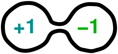
(a)	(b)

Figure 1. (a) Schematic representation of a dynamical system with almost-invariant regions. (b) Approximate values of eigenfunction corresponding to the bottleneck.

While this Ansatz was initially made in the context of a single dynamical system, it seems to apply equally in the case of random dynamical systems [11, 12, 6], and this is the central motivation for our research in this area. It is well known that Perron-Frobenius operators of non-invertible maps are essentially never invertible, but it is often reasonable to assume that the base dynamics are invertible. Indeed, even if the driving system is non-invertible, one can make use of canonical mathematical techniques to extend it to an invertible one. Hence, we naturally find ourselves in the semi-invertible category. The principal object that we are interested in understanding is the second Oseledets subspace (or more generally the first few Oseledets subspaces).

The significance of our extensions to the MET is that the second subspace that we obtain is low-dimensional (typically one-dimensional) instead of $(d-1)$-dimensional, which is what would come from the standard non-invertible MET. In numerical applications, where $d$ may be $10^{5}$ or greater, one cannot expect to say anything reasonable about level sets of functions belonging to a high-dimensional subspace, whereas using the semi-invertible version of the theorem, we are once again in a position to make sense of the level sets.

In practice, of course, one cannot numerically study the action of Perron-Frobenius operators on infinite-dimensional Banach spaces. Nor can one find a finite-dimensional subspace preserved by the operators. A remarkably fruitful approach is the so-called Ulam method. Here, the state space is cut into small reasonably regular pieces and a single dynamical system is treated as a Markov chain, by applying the dynamical system and then randomizing over the cell in which the point lands. This also makes sense for random dynamical systems.

In [8], we showed that applying the Ulam method to certain random dynamical systems, the top Oseledets space of the truncated system converges in probability to the true top Oseledets space of the random dynamical system as the size of the partition is shrunk to 0. The top Oseledets space is known to correspond to the random absolutely continuous invariant measure of the system. It is natural to ask whether the subsequent Oseledets spaces for the truncated systems converge to the corresponding Oseledets spaces for the full system. We are not yet able to answer this, although the current paper represents a substantial step in this direction.

In [8], we viewed the Ulam projections of the Perron-Frobenius operator as perturbations of the original operator, and showed that the top Oseledets space was robust to the kind of projections that were being considered. In this paper, we prove convergence the of subsequent Oseledets spaces under certain perturbations, but do this in the context of matrices instead of infinite-dimensional operators.

In general, Lyapunov exponents and Oseledets subspaces are known to be highly sensitive to perturbations. A mechanism responsible for this is attributed to Mañé; see also [2]. Ledrappier and Young considered the case of perturbations of random products of uniformly invertible matrices [15]. This followed related work of Young in the two-dimensional setting [18]. In view of the sensitivity results, it was necessary to restrict the class of perturbations that they considered, and they dealt with the situation where the distribution of the perturbation of the matrix at time 0 was absolutely continuous (with control on the density) conditioned on all previous perturbations. The simplest instance of this is the case where the matrices to be multiplied are subjected to additive i.i.d. absolutely continuous noise. In this situation, they showed that the perturbed exponents converge almost surely to the true exponents as the noise is shrunk to 0. While they did not directly address the Oseledets subspaces, work of Ochs shows that convergence of the Lyapunov exponents implies convergence in probability of the Oseledets subspaces [16].

In this paper, we deal with the case of uniform i.i.d. additive noise in the matrices, but make no assumption on invertibility. The conclusions that we obtain are the same as may be obtained in the invertible case. Our argument first demonstrates stability of the Lyapunov exponents, and then shows stability of the Oseledets subspaces. The first part is closely based on Ledrappier and Young’s approach, although we need to do some non-trivial extra work to deal with the lack of uniform invertibility (in Ledrappier-Young’s argument, in one step, there is an upper bound to the amount of damage that can be done to the exponents, whereas in the non-invertible case there is no such bound). The second part of the argument is completely new. The methods of Ochs cannot be made to work here because they are based on finding the space with the smallest exponent and then using tensor products to move up the ladder. In the case where the smallest exponent is $-\infty$, when one takes tensor products, all products with this subspace have exponent $-\infty$ so there is no distinguished second-smallest subspace. To get around this problem, we use the Grassmannian in place of the exterior algebra. We study evolution of subspaces in the Grassmannian, and show that this is controlled by fractional linear transformations. An important role is played by a higher-dimensional analogue of the cross ratio.

We are hopeful that the techniques that we introduce to control evolution of these Oseledets subspaces under the matrices may be applied much more widely.

1.1. Statements of the main results

If $\sigma\colon(\Omega,\mathbb{P})\to(\Omega,\mathbb{P})$ is a measure-preserving transformation of a probability space and $A\colon\Omega\to M_{d\times d}(\mathbb{R})$ is a measurable matrix-valued function, we let $A^{(n)}_{\omega}$ denote the product $A(\sigma^{n-1}\omega)A(\sigma^{n-2}\omega)\cdots A(\omega)$. We call the tuple $(\Omega,\mathbb{P},\sigma,A)$ a matrix cocycle.

Let $U=\{A\in M_{d\times d}(\mathbb{R})\colon\|A\|\leq 1\}$ (here and throughout the paper, the norm of a matrix is its operator norm). Let $\bar{\Omega}=\Omega\times U^{\mathbb{Z}}$. We write $\bar{\omega}=(\omega,\Delta)$ for a typical element of $\bar{\Omega}$. If $\Omega$ is equipped with the measure $\mathbb{P}$, we equip $\bar{\Omega}$ with the measure $\bar{\mathbb{P}}=\mathbb{P}\times\lambda^{\mathbb{Z}}$, where $\lambda$ is the uniform measure on $U$ and $\lambda^{\mathbb{Z}}$ is the product measure. We fix an $\epsilon>0$. Then for an element $\bar{\omega}\in\bar{\Omega}$, the corresponding sequence of matrices is $(A^{\epsilon}_{n}(\bar{\omega}))_{n\in\mathbb{Z}}=(A(\sigma^{n}\omega)+\epsilon\Delta_{n})_{n\in\mathbb{Z}}$. This paper is concerned with a comparison of the properties of the matrix cocycle $(\Omega,\mathbb{P},\sigma,A)$ with those of the matrix cocycle $(\bar{\Omega},\bar{\mathbb{P}},\bar{\sigma},A^{\epsilon})$ as $\epsilon\to 0$.

The main result of this paper is the following.

Theorem 1.

Let $\sigma$ be an ergodic measure-preserving transformation of $(\Omega,\mathbb{P})$ and let $A\colon\Omega\to M_{d\times d}(\mathbb{R})$ be a measurable map such that $\int\log^{+}\|A(\omega)\|\,d\mathbb{P}(\omega)<\infty$.

Let the Lyapunov exponents of the matrix cocycle be $\lambda_{1}>\ldots>\lambda_{p}\geq-\infty$ with multiplicities $d_{1},d_{2},\ldots,d_{p}$ and let the corresponding Oseledets decomposition be $\mathbb{R}^{d}=Y_{1}(\omega)\oplus\ldots\oplus Y_{p}(\omega)$.

Let $D_{0}=0$, $D_{i}=d_{1}+\ldots+d_{i}$ and let the Lyapunov exponents (with multiplicity) be $\infty>\mu_{1}\geq\mu_{2}\geq\ldots\geq\mu_{d}\geq-\infty$, so that $\mu_{i}=\lambda_{k}$ if $D_{k-1}<i\leq D_{k}$.

1. (Convergence of Lyapunov exponents) Let the Lyapunov exponents of the perturbed matrix cocycle $(\bar{\Omega},\bar{P},\bar{\sigma},A^{\epsilon})$ (with multiplicity) be $\mu_{1}^{\epsilon}\geq\mu_{2}^{\epsilon}\geq\ldots\geq\mu_{d}^{\epsilon}$. Then $\mu_{i}^{\epsilon}\to\mu_{i}$ for each $i$ as $\epsilon\to 0$.

2. (Convergence in probability of Oseledets spaces) Let $\tau=\frac{1}{12}\min_{1\leq i<j}(\lambda_{i}-\lambda_{i+1})$. Let $\epsilon_{0}$ be such that $|\mu_{i}^{\epsilon}-\mu_{i}|<\tau$ for each $i$ for all $\epsilon\leq\epsilon_{0}$. For $\epsilon<\epsilon_{0}$, let $Y^{\epsilon}_{i}(\omega)$ denote the sum of the Lyapunov subspaces having exponents in the range $(\lambda_{i}-\tau,\lambda_{i}+\tau)$. Then $Y^{\epsilon}_{i}(\bar{\omega})$ converges in probability to $Y_{i}(\omega)$ as $\epsilon\to 0$.

1.2. Outline of the paper

Section 2 introduces terminology, background results and a collection of lemmas that will be used in the proof of the main result. Theorem 1(I) is established in Section 3, and part (II) is proven in Section 4.

2. Preliminaries

For two subspaces, $U$ and $V$, of $\mathbb{R}^{d}$ of the same dimension, we define $\angle(U,V)=d_{H}(U\cap B,V\cap B)$, where $d_{H}$ denotes Hausdorff distance and $B$ is the unit ball. For two subspaces $U$ and $W$ of complementary dimensions, we define $\perp(U,W)=(1/\sqrt{2})\inf_{\{u\in U\cap S,\,w\in W\cap S\}}\|u-w\|$, where $S$ denotes the unit sphere. Thus $\perp(U,W)$ is a measure of complementarity of subspaces, taking values between 0 and 1, with 0 indicating that the spaces intersect and 1 indicating that the spaces are orthogonal complements. Note that $\perp(U,V)\geq\perp(U,W)-\angle(W,V)$.

Let $s_{j}(A)$ denote the $j$th singular value of the matrix $A$ and let $\Xi^{j}(A)$ denote $\log s_{1}(A)+\ldots+\log s_{j}(A)$. Note that $\Xi^{j}(A)=\log\|\Lambda^{j}A\|$, so that $\Xi^{j}(AB)\leq\Xi^{j}(A)+\Xi^{j}(B)$.

The structure of the proof of the main theorem closely follows that of Ledrappier and Young, in which the orbit of $\omega$ is divided into blocks of length $\approx|\log\epsilon|$. These are classified as good if a number of conditions hold (separation of Lyapunov spaces, closeness of averages to integrals etc.) and bad otherwise. The crucial modifications that we make are in estimations for the bad blocks. In the case of [15], the matrices (and hence their perturbations) have uniformly bounded inverses, so that for bad blocks one can give uniform lower bounds on the contribution to the singular value. By contrast, here, there is no uniform lower bound. Upper bounds are straightforward, so all of the work is concerned with establishing lower bounds for the exponents. Absent the invertibility, a similar argument would yield (random) bounds of order $\log\epsilon$, which turn out to be too weak to give the lower bounds that we need.

Given a matrix $A$ with the property that $s_{j+1}(A)<s_{j}(A)$, we define $E_{j}(A)$ to be the space spanned by the $(j+1)$st to $d$th singular vectors and $F_{j}(A)$ to be the space spanned by the images of the 1st to $j$th singular vectors under $A$. If one has a matrix cocycle with base space $\Omega$ and matrices $A_{\omega}$, we use the very similar notation $E_{j}(\omega)$ and $F_{j}(\omega)$ to refer to the Oseledets subspaces. The convention will be that if the argument is a matrix, then they refer to the span of the bottom singular vectors or the images of the top singular vectors, while if the argument is a point of the base space, they refer to spaces appearing in the Oseledets theorem. These spaces are obtained simply as limits of spans of singular vectors, as explained in Lemma 2 below, justifying the notation.

Lemma 2 (Singular Vectors of blocks of the unperturbed system).

Suppose that the unperturbed system has exponents satisfying $\lambda_{j}>\lambda_{j+1}$.

Then for almost every $\omega$, $E_{j}(A^{(n)}_{\omega})\to E_{j}(\omega)$ and $F_{j}(A^{(n)}_{\sigma^{-n}\omega})\to F_{j}(\omega)$ as $n\to\infty$.

Proof.

The statement that $E_{j}(A^{(n)}_{\omega})\to E_{j}(\omega)$ follows from the proof of Oseledets’ theorem given in [1]. The singular value decomposition ensures that $F_{j}(A^{(n)}_{\sigma^{-n}\omega})=\Big{(}E_{j}(A^{(n)\,*}_{\sigma^{-n}\omega})\Big{)}^{\perp}$, where $A^{*}$ denotes the adjoint of $A$.

On the other hand, a similar statement is true for the spaces $E^{*}_{j}(\omega)$ and $F_{j}(\omega)$. More precisely, we claim that if we let $E^{*}_{j}(\omega)$ be the Oseledets spaces for the dual cocycle with base $\sigma^{-1}$ and generator $G(\omega)={A(\sigma^{-1}\omega)}^{*}$, then $F_{j}(\omega)=(E^{*}_{j}(\omega))^{\perp}$. Applying Oseledets’ theorem to the dual cocycle, we obtain $E_{j}(A^{(n)\,*}_{\sigma^{-n}\omega})\to E^{*}_{j}(\omega)$.

To prove the claim, suppose for a contradiction that there exist $f(\omega)\in F_{j}(\omega)$ and $e^{*}(\omega)\in E^{*}_{j}(\omega)$ of unit length such that $\langle f(\omega),e^{*}(\omega)\rangle\neq 0$. By invertibility of $A^{(n)}_{\sigma^{-n}\omega}$ as a map from $F_{j}(\sigma^{-n}\omega)$ to $F_{j}(\omega)$ there exist for all $n$, unit vectors $f^{(-n)}(\omega)\in F_{j}(\sigma^{-n}\omega)$ such that $A^{(n)}_{\sigma^{-n}\omega}f^{(-n)}(\omega)$ is a multiple of $f(\omega)$. Then,

(1) $$\langle A^{(n)}_{\sigma^{-n}\omega}f^{(-n)}(\omega),e^{*}(\omega)\rangle=\langle f^{(-n)}(\omega),A^{(n)\,*}_{\sigma^{-n}\omega}e^{*}(\omega)\rangle.$$

The right hand side grows at a rate slower than $\lambda_{j}$. The left hand side grows at a rate at least $\lambda_{j}$, by [9, Eq. (18)]. This yields a contradiction, so $F_{j}(\omega)\subset\big{(}E^{*}_{j}(\omega)\big{)}^{\perp}$. Since the dimensions agree, they coincide.

Now the statement that $F_{j}(A^{(n)}_{\sigma^{-n}\omega})\to F_{j}(\omega)$ follows directly from the fact that $E_{j}(A^{(n)\,*}_{\sigma^{-n}\omega})\to E^{*}_{j}(\omega)$, and continuity of $V\mapsto V^{\perp}$.

∎

Lemma 3.

[Lemmas 3.3, 3.6 & 4.3, [15]] For any $\delta>0$, there exists a $K$ such that if (i) the ratio of the $j$th to $(j+1)$st singular values of a matrix $A$ exceeds $K$; (ii) the $j$th singular value exceeds $K$; and (iii) $\|B-A\|\leq 1$, then the following hold:

1. $\angle(F_{j}(A),F_{j}(B))$ and $\angle(E_{j}(A),E_{j}(B))$ are less than $\delta/3$;

2. $\frac{1}{3}\leq s_{i}(A)/s_{i}(B)\leq 3$ for each $i\leq j$;

3. If $V$ is any subspace of dimension $j$ such that $\perp(V,E_{j}(A))>\delta/6$, then $\angle(BV,F_{j}(A))<\delta/3$;

4. If $V$ is a subspace of dimension $j$ and $\perp(V,E_{j}(A))>\delta$, then $|\det(A|V)|\geq(D\delta)^{j}\exp\Xi_{j}(A)$, where $D$ is an absolute constant.

Lemma 4.

Let $\sigma$ be an ergodic measure-preserving transformation of $(\Omega,\mathbb{P})$ and let $A\colon\Omega\to M_{d\times d}(\mathbb{R})$ be a measurable map such that $\log^{+}\|A(\omega)\|$ is integrable. There exists $C$ such that for all $\eta_{0}>0$, there exists $\epsilon_{0}$ such that for all $\epsilon<\epsilon_{0}$, there exists $G\subseteq\Omega$ of measure at least $1-\eta_{0}$ such that for all $\omega\in G$, and all $(\Delta_{n})\in U^{\mathbb{Z}}$

$$\|{A^{\epsilon}}^{(N)}_{(\omega,(\Delta_{n}))}-A^{(N)}_{\omega}\|\leq 1,$$

where $N=\lfloor C|\log\epsilon|\rfloor$.

Proof.

Let $g(\omega)=\log^{+}(\|A_{\omega}\|+1)$ and let $C>0$ satisfy $\int g(\omega)\,d\mathbb{P}(\omega)<1/C$. Notice that provided $\epsilon<1$ (and using the fact that the perturbations have norm bounded by $\epsilon$), $\log^{+}\|A_{\bar{\omega}}^{\epsilon}\|\leq g(\omega)$, and

$$\|{A^{\epsilon}}^{(N)}_{\bar{\omega}}-A^{(N)}_{\omega}\| \leq\sum_{i=0}^{N-1}\|{A^{\epsilon}}^{(N-i-1)}_{\bar{\sigma}^{i}\bar{\omega}}(A^{\epsilon}_{\bar{\sigma}^{i}\bar{\omega}}-A_{\sigma^{i}\omega})A^{(i)}_{\omega}\|$$

$$\leq N\epsilon\exp(g(\omega)+\ldots+g(\sigma^{N-1}\omega)).$$

There exists $n_{0}$ such that for $N\geq n_{0}$, $N\epsilon\exp(g(\omega)+\ldots+g(\sigma^{N-1}\omega))\leq\epsilon\exp(N/C)$ on a set of measure at least $1-\eta_{0}$. In particular, provided $\lfloor C|\log\epsilon_{0}|\rfloor>n_{0}$, taking $N=\lfloor C|\log\epsilon|\rfloor$, the conclusion follows.

∎

Lemma 5.

Let $\sigma$ be an ergodic measure-preserving transformation of $(\Omega,\mathbb{P})$ and let $A\colon\Omega\to M_{d\times d}(\mathbb{R})$ be a measurable map such that $\int\log^{+}\|A(\omega)\|\,\mathbb{P}(\omega)<\infty$. Let the Lyapunov exponents (with multiplicity) be $\infty>\mu_{1}\geq\ldots\geq\mu_{d}\geq-\infty$. Suppose further that $\mu_{j}>\max(0,\mu_{j+1})$.

Let $\eta_{0}>0$ and $\delta_{1}>0$ be given. Then there exist $n_{0}>0$, $\kappa>0$ and $\delta\leq\min(\delta_{1},\kappa)$ such that: for all $n\geq n_{0}$, there exists a set $G\subseteq\Omega$ with $\mathbb{P}(G)>1-\eta_{0}$ such that for $\omega\in G$, we have

1. $\perp(E_{j}(\omega),F_{j}(\omega))>10\kappa$;

2. $\angle(F_{j}(A^{(n)}_{\omega}),F_{j}(\sigma^{n}\omega))<\delta$;

3. $\angle(E_{j}(A^{(n)}_{\omega}),E_{j}(\omega))<\delta$;

4. $s_{j}(A^{(n)}_{\omega})/s_{j+1}(A^{(n)}_{\omega})>K(\delta)$ and $s_{j}(A^{(n)}_{\omega})>K(\delta)$, where $K(\delta)$ is as given in Lemma 3.

Proof.

From the proof of Oseledets’ theorem, we know $\perp(E_{j}(\omega),F_{j}(\omega))$ is a positive measurable function. Hence there exists $\kappa>0$ such that (a) occurs on a set of measure at least $1-\eta_{0}/4$. Let $\delta=\min(\delta_{1},\kappa)$.

From the proof of Oseledets’ theorem, there exists an $n_{1}>0$ such that for all $n\geq n_{1}$, $\angle(F_{j}(A^{(n)}_{\sigma^{-n}\omega}),F_{j}(\omega))<\delta$ and $\angle(E_{j}(A^{(n)}_{\omega}),E_{j}(\omega))<\delta$ hold on sets of measure at least $1-\eta_{0}/4$. Hence there is a set of measure at least $1-\eta_{0}/4$ where (c) holds. Similarly, using shift-invariance, there is a set of measure at least $1-\eta_{0}/4$ where (b) holds.

Since $\frac{1}{n}\log s_{j}(A^{(n)}_{\omega})\to\mu_{j}$ and $\frac{1}{n}\log s_{j+1}(A^{(n)}_{\omega})\to\mu_{j+1}$, (d) holds on a set of measure at least $1-\eta_{0}/4$ for all $n\geq n_{2}$ for some $n_{2}>0$. Now let $n\geq n_{0}=\max(n_{1},n_{2})$. Intersecting the above sets gives a set $G$ satisfying the conclusions of the lemma. ∎

3. Convergence of Lyapunov exponents

Proof of Theorem 1(I).

Most of the work in this part is concerned with showing the inequality

(2) $$\liminf_{\epsilon\to 0}(\mu_{1}^{\epsilon}+\ldots+\mu_{D_{i}}^{\epsilon})\geq\mu_{1}+\ldots+\mu_{D_{i}}\text{, for any $1\leq i\leq p$}.$$

We also prove

(3) $$\limsup_{\epsilon\to 0}(\mu_{1}^{\epsilon}+\ldots+\mu_{j}^{\epsilon})\leq\mu_{1}+\ldots+\mu_{j}\text{ for any $1\leq j\leq d$}$$

which is fairly straightforward using sub-additivity. These facts, combined with the fact that the $\mu_{i}^{\epsilon}$ and $\mu_{i}$ are decreasing in $i$ are sufficient to establish the claim that $\mu_{i}^{\epsilon}\to\mu_{i}$ for each $i$.

To see this, suppose that (2) and (3) hold. Let $h_{j}=\mu_{1}+\ldots+\mu_{j}$ and let $H_{j}(\epsilon)=\mu_{1}^{\epsilon}+\ldots+\mu_{j}^{\epsilon}$. By (2) and (3), we have $\lim_{\epsilon\to 0}H_{D_{i}}(\epsilon)=h_{D_{i}}$. If $\lambda_{i+1}=-\infty$, we see $\lim_{\epsilon\to 0}\mu_{j}^{\epsilon}=-\infty$ for all $j>D_{i}$ from (3). Hence we may assume that $\lambda_{i+1}>-\infty$. Since the exponents are arranged in decreasing order, $(H_{j}(\epsilon))_{j=1}^{d}$ is a ‘concave’ sequence for each $\epsilon$ (that is $H_{j+1}(\epsilon)-H_{j}(\epsilon)\leq H_{j}(\epsilon)-H_{j-1}(\epsilon)$ for each $j$ in range), as is $(h_{j})_{j=1}^{d}$. However, $h_{j}$ is an arithmetic progression for $j$ in the range $D_{i}$ to $D_{i+1}-1$. Since a concave function is bounded below by its secant, we deduce $\liminf_{\epsilon\to 0}H_{j}(\epsilon)\geq h_{j}$ for $D_{i}\leq j<D_{i+1}$. Hence we see $H_{j}(\epsilon)\to h_{j}$ as $\epsilon\to 0$ for each $j$, from which the statement follows.

To show (3), let $\chi>0$ and let $1\leq j\leq d$. By the sub-additive ergodic theorem, there exists an $N>0$ such that $\int\Xi_{j}(A^{(N)}_{\omega})\,d\mathbb{P}<h_{j}+\chi/2$. Now for sufficiently small $\epsilon>0$, $\Xi_{j}({A^{\epsilon}}^{(N)}_{\bar{\omega}})<\Xi_{j}(A^{(N)}_{\omega})+\chi/2$ for all $\bar{\omega}\in\bar{\Omega}$. In particular, this shows that $H_{j}(\epsilon)<h_{j}+\chi$ for all sufficiently small $\epsilon$ as required. Notice that this part of the argument is completely general, whereas the lower bound depends on the particular properties of the matrix perturbations.

We now focus on proving (2). Let $j=D_{i}$, noting that by the above, we may assume that $\lambda_{i}>-\infty$. By multiplying the entire family of matrices by a positive constant, we may assume that $\mu_{j}=\lambda_{i}\geq 0$.

Let $\chi>0$ be arbitrary. Let $D$ be the absolute constant occurring in the statement of Lemma 3, $C$ be as in the statement of Lemma 4 and $K$ be the constant occurring in the statement of Lemma 10. Define a constant $\eta>0$ by

(4) $$\eta=\min\left(\frac{\chi}{4\times 1.28d^{2}j},\frac{\chi C}{8K}\right).$$

Let $n_{0}$, $\kappa$ and $\delta$ be the quantities given by Lemma 5 using $\delta_{1}=\frac{1}{2}$ and $\eta_{0}=\eta/2$. Since $\int\log\|A_{\omega}\|\,d\mathbb{P}(\omega)<\infty$, it follows that $\int\Xi_{j}^{+}(A_{\omega})\,d\mathbb{P}(\omega)<\infty$.

Let $N(\epsilon)=\lfloor C|\log\epsilon|\rfloor$, where $C$ is as above. The fact that $N$ scales like $|\log\epsilon|$ will be of crucial importance later. Let $\epsilon_{0}$ be the quantity appearing in Lemma 4 with $\eta_{0}$ taken to be $\eta/2$.

Let $\epsilon$ be sufficiently small that

(5) $$\begin{split}N(\epsilon)&>\frac{4j\log(3/(\delta D))}{\chi},\\ \frac{|\log\epsilon|}{N(\epsilon)}&<2/C,\\ N(\epsilon)&>\frac{8}{\chi}\int\Xi_{j}^{+}(A_{\omega})\,d\mathbb{P}(\omega),\\ \epsilon&<\epsilon_{0}.\end{split}$$

Let $G$ be the intersection of the good set given by Lemma 4 with the good set given by Lemma 5 with $n$ taken to be $N=N(\epsilon)$, so that $\mathbb{P}(G)>1-\eta$. If $\omega\in G$, we say the matrix product $A_{\sigma^{N-1}\omega}\cdots A_{\omega}$ is a good block.

Now we divide everything into blocks of length $N$ and estimate the sum of the logarithms of the first $j$ singular values of the $\epsilon$-perturbed cocycle.

We will bound from above the difference between the sum of the logs of the first $j$ singular values in the unperturbed system and this sum in the perturbed version. We informally speak of the costs due to various contributions. That is, estimates of various contributions to an upper bound for the difference (unperturbed)$-$(perturbed). These costs are estimated in the following parts.

1. To deal with the concatenation of good blocks, we give an upper bound for the difference (sum of individual block exponents)$-$(exponent of concatenated block). This is estimated using Lemma 3. Over the whole block there is a cost of at most $\log(3/D\delta)$, so a cost per index of $O(1/|\log\epsilon|)$.

2. Reduction of singular values within bad blocks. There is an expected cost of at worst $1.28d^{2}j$ per index in a bad block from (8).

3. Reduction of singular values at the first and last matrix of a string of bad blocks. Here, there is an upper bound in expected cost of approximately $|\log\epsilon|$ per bad block. Here is where it is crucial that the blocks are of length $O(|\log\epsilon|)$. The upper bound for the cost averages out at $O(1)$ per index in each bad block. The argument is saved by the fact that most blocks are good blocks.

The sum of the costs is $O(\eta)+O(1/|\log\epsilon|)$ per index ($\eta$ being the frequency of bad blocks), which will allow us to derive (2). Let us proceed with the details.

Step 1.

A lower bound for $\Xi_{j}$ for concatenations of good blocks.

Suppose $k<l$ and $\sigma^{kN}\omega,\sigma^{(k+1)N}\omega,\ldots,\sigma^{(l-1)N}\omega\in G$. Let $B_{n}=A^{(N)}_{\sigma^{nN}\omega}$ and $\tilde{B}_{n}={A^{\epsilon}}^{(N)}_{\sigma^{nN}\omega}$ We then claim that

(6) $$\begin{split}\Xi_{j}(\tilde{B}_{l-1}\cdots\tilde{B}_{k})&\geq\sum_{i=k}^{l-1}\Xi_{j}(B_{i})+(l-k)j\log\delta-(l-k)j\log(3/D)\\ &\geq\Xi_{j}(B_{l-1}\cdots B_{k})+(l-k)j\log(D\delta/3),\end{split}$$

where $D$ is the absolute constant appearing in Lemma 3.

This is proved inductively using Lemma 3. Recall that $\|B_{n}-\tilde{B}_{n}\|\leq 1$. We let $\tilde{V}_{k}=V_{k}=E_{j}(B_{k})^{\perp}$ and define $V_{n+1}=B_{n}V_{n}$ and $\tilde{V}_{n+1}=\tilde{B}_{n}\tilde{V}_{n}$.

We claim that the following hold:

1. $\angle(V_{n},\tilde{V}_{n})<\delta$ for each $n$;

2. $\perp(V_{n},E_{j}(B_{n}))>\delta$ and $\perp(\tilde{V}_{n},E_{j}(\tilde{B}_{n}))>\delta$ for each $n$.

Item (i) and the first part of (ii) hold immediately for the case $n=k$. The second part of (ii) holds because $\tilde{V}_{k}=V_{k}=E_{j}(B_{k})^{\perp}$ and $\angle(E_{j}(B_{k}),E_{j}(\tilde{B}_{k}))<\delta$ by Lemma 3.

Given that (i) and (ii) hold for $n=m$ and that $B_{m}$ is a good block, Lemma 3 implies that $\angle(V_{m+1},F_{j}(B_{m}))<\delta/3$, $\angle(\tilde{V}_{m+1},F_{j}(\tilde{B}_{m}))<\delta/3$ and $\angle(F_{j}(B_{m}),F_{j}(\tilde{B}_{m}))<\delta/3$, so that $\angle(\tilde{V}_{m+1},V_{m+1})<\delta$, yielding (i) for $n=m+1$.

Finally, by the induction hypothesis and Lemma 3, we have $\angle(F_{j}(\sigma^{(m+1)N}\omega),F_{j}(B_{m}))<\delta$, and by Lemma 5, $\perp(F_{j}(\sigma^{(m+1)N}\omega),E_{j}(\sigma^{(m+1)N}\omega))>10\delta$. Thus, we obtain (ii) for $n=m+1$.

Hence using Lemma 3(d), we see that $\text{det}(\tilde{B}_{n}|_{\tilde{V}_{n}})\geq(D\delta)^{j}\det(\tilde{B}_{n}|_{E_{j}(\tilde{B}_{n})^{\perp}})=(D\delta)^{j}e^{\Xi_{j}(\tilde{B}_{n})}\geq(D\delta/3)^{j}e^{\Xi_{j}(B_{n})}$.

Since $\Xi_{j}(\tilde{B}_{l-1}\cdots\tilde{B}_{k})\geq\prod_{i=k}^{l-1}\det(\tilde{B}_{i}|\tilde{V}_{i})$, multiplying the inequalities and taking logarithms gives the result.

Step 2.

A lower bound for $\Xi_{j}$ for concatenations of arbitrary blocks.

Let $A_{1},\ldots,A_{n}$ be an arbitrary sequence of matrices. We write

(7) $$g^{\epsilon}(A_{1},\ldots,A_{n},\Delta_{1},\ldots,\Delta_{n})=\Xi_{j}(A^{\epsilon}_{n}\ldots A^{\epsilon}_{1})-\Xi_{j}(A_{n}\ldots A_{1})$$

and prove that $(g^{\epsilon})^{-}$ is integrable in $\Delta_{1},\ldots,\Delta_{n}$ and that

(8) $$\int g^{\epsilon}(A_{1},\ldots,A_{n},\Delta_{1},\ldots,\Delta_{n})\,d\lambda^{n}(\Delta_{1},\ldots,\Delta_{n})\geq-1.28d^{2}nj$$

for all $A_{1},\ldots,A_{n}$.

Lemma 6.

There exists $B\approx-1.28$ such that for all $z\in\mathbb{C}$, and all $l\geq 0$

$$\int_{0}^{1}t^{l}\log|1-tz|\,dt\geq B.$$

Proof.

Let us show there exists a lower bound; its precise value is irrelevant for our purposes. Since for every $z\in\mathbb{C},t\in[0,1]$, we have that $|1-tz|\geq|1-tRe(z)|\geq\big{|}1-t|Re(z)|\big{|}$, it suffices to show the lemma holds for $z\in\mathbb{R}^{+}\cup\{0\}$. For $z=0$ the integral is 0. Let us assume $z\in\mathbb{R}^{+}$, and let $\log^{-}x:=\min(0,\log x)$. Then,

$$\int_{0}^{1}t^{l}\log|1-tz|\,dt \geq\int_{0}^{1}t^{l}\log^{-}|1-tz|\,dt\geq\int_{0}^{1}\log^{-}|1-tz|\,dt$$

$$=\frac{1}{z}\int_{0}^{z}\log^{-}|1-y|\,dy\geq\inf_{z\in(0,2]}\frac{1}{z}\int_{0}^{z}\log^{-}|1-y|\,dy.$$

The function $g(z):=\frac{1}{z}\int_{0}^{z}\log^{-}|1-y|\,dy$ for $z\neq 0$ and $g(0):=0$ is continuous on $\mathbb{R}^{+}$, and hence bounded on $[0,2]$. The statement follows. ∎

Lemma 7.

Let $B$ be as in Lemma 6 and $p$ be a polynomial. Then, for all $l\geq 0$,

$$\int_{0}^{1}t^{l}(\log|p(t)|-\log|p(0)|)\,dt\geq B\cdot\deg(p).$$

Proof.

If $p(0)=0$, then the result is clear. Otherwise, we consider the polynomial $f(t)=p(t)/p(0)$ and demonstrate that $\int_{0}^{1}t^{l}\log|f(t)|\,dt\geq B\cdot\text{deg}(f)$.

To see this, notice that $f(t)$ may be expressed as $\prod_{i=1}^{\text{deg}(f)}(1-tz_{i})$, where $\{z_{i}^{-1}\}_{i=1}^{\text{deg}(f)}$ is the set of roots of $f$, and hence $p$, with multiplicity. Applying Lemma 6 then gives the result. ∎

Lemma 8.

Let $B$ be the constant from the statement of Lemma 6. Let $P(t)$ be a degree $j$ matrix-valued polynomial. That is, $P(t)$ may be expressed as $\sum_{k=0}^{j}A_{k}t^{k}$ for some collection of $d\times d$ matrices $A_{k}$. Then, for all $l\geq 0$,

$$\int_{0}^{1}t^{l}(\log\|P(t)\|-\log\|P(0)\|)\,dt\geq B\cdot\deg(P).$$

Proof.

If $P(0)$ is the zero matrix, the result is trivial. Otherwise, there exist unit vectors $\mathbf{e}$ and $\mathbf{f}$ such that $P(0)\mathbf{e}=\|P(0)\|\mathbf{f}$.

If we set $p(t)=\langle P(t)\mathbf{e},\mathbf{f}\rangle$, then we have $p(0)=\|P(0)\|$ and $\|P(t)\|\geq|p(t)|$, so the result follows from Lemma 7. ∎

Lemma 9.

Let $B\approx-1.28$ be the constant from the statement of Lemma 6. Let $L$, $M$, $A$ and $R$ be arbitrary $d\times d$ matrices. Then

$$\int_{0}^{1}t^{l}\left(\log\|\Lambda^{j}(L(A+tM)R)\|-\log\|\Lambda^{j}(LAR)\|\right)\,dt\geq jB.$$

Proof.

Notice that $\Lambda^{j}(L(A+tM)R)$ is a polynomial family of operators on $\Lambda^{j}\mathbb{R}^{d}$. Taking the standard orthogonal basis of $\Lambda^{j}\mathbb{R}^{d}$, let $P(t)$ be the matrix of $\Lambda^{j}(L(A+tM)R)$. The result then follows by applying Lemma 8. ∎

We obtain (8) by a telescoping argument:

$$\Xi_{j}(A_{n}\ldots A_{1})-\Xi_{j}(A_{n}^{\epsilon}\ldots A_{1}^{\epsilon})$$

$$=\sum_{k=1}^{n}\left(\Xi_{j}(A_{n}^{\epsilon}\ldots A_{k+1}^{\epsilon}A_{k}\ldots A_{1})-\Xi_{j}(A_{n}^{\epsilon}\ldots A_{k}^{\epsilon}A_{k-1}\ldots A_{1})\right)$$

Recall that $\Xi_{j}(A)=\log\|\Lambda^{j}A\|$. We estimate the integral of the $k$th term in the sum. Let $L=A_{n}^{\epsilon}\ldots A_{k+1}^{\epsilon}$ and $R=A_{k-1}\ldots A_{1}$. Regarding $\Delta_{k+1},\ldots,\Delta_{n}$ as fixed, we need to estimate:

$$\int_{\mathbf{B}}\left(\log\|\Lambda^{j}(LA_{k}R)\|-\log\|\Lambda^{j}(L(A_{k}+\epsilon\Delta)R)\|\right)\,d\lambda(\Delta),$$

where $\mathbf{B}=\{M\colon\|M\|\leq 1\}$. We then disintegrate the measure $\lambda$ radially, so that $d\lambda=d^{2}t^{d^{2}-1}\,dt\cdot d(\partial\lambda)(H)$ where $\Delta=tH$, $H$ takes values in $\partial\mathbf{B}$ and $\partial\lambda$ is the boundary measure. For a fixed $H$, the quantity to estimate is

$$\int_{0}^{1}\left(\log\|\Lambda^{j}(LA_{k}R)\|-\log\|\Lambda^{j}(L(A_{k}+\epsilon tH)R)\|\right)t^{d^{2}-1}\,dt.$$

Since this quantity is uniformly bounded above, by Lemma 9, we obtain (8).

Step 3.

Gluing blocks.

Lemma 10.

Let $L$, $R$ and $A$ be given matrices. Then $\Xi_{j}(L(A+\epsilon\Delta)R)-(\Xi_{j}(L)+\Xi_{j}(R))$ is has integrable negative part as a function of $\Delta$ and has integral bounded below by $K\log\epsilon$, where $K$ is independent of $L$, $A$ and $R$.

Proof.

Write $L=O_{1}D_{1}O_{2}$ where $D_{1}$ is diagonal with entries arranged in decreasing order and $O_{1}$ and $O_{2}$ are orthogonal. Similarly write $R=O_{3}D_{2}O_{4}$. Let $A^{\prime}=O_{2}AO_{3}$ and $\Delta^{\prime}=O_{2}\Delta O_{3}$. Then we have

$$\Xi_{j}(L(A+\epsilon\Delta)R) =\Xi_{j}(D_{1}(A^{\prime}+\epsilon\Delta^{\prime})D_{2});$$

$$\Xi_{j}(L) =\Xi_{j}(D_{1});\text{ and }$$

$$\Xi_{j}(R) =\Xi_{j}(D_{2}).$$

Using the inequality $\Xi_{j}(AB)\leq\Xi_{j}(A)+\Xi_{j}(B)$ and setting $C$ to be the diagonal matrix with 1’s in the first $j$ elements of the diagonal and 0’s elsewhere, we have

$$\Xi_{j}(D_{1}(A^{\prime}+\epsilon\Delta^{\prime})D_{2}) \geq\Xi_{j}(CD_{1}(A^{\prime}+\epsilon\Delta^{\prime})D_{2}C)$$

$$=\Xi_{j}(D_{1}C(A^{\prime}+\epsilon\Delta^{\prime})CD_{2})$$

$$=\Xi_{j}(D_{1}C)+\Xi_{j}(C(A^{\prime}+\epsilon\Delta^{\prime})C)+\Xi_{j}(CD_{2})$$

$$=\Xi_{j}(L)+\Xi_{j}(R)+\Xi_{j}(C(A^{\prime}+\epsilon\Delta^{\prime})C).$$

The equality between the second and third lines arises because the matrices $D_{1}C$, $C(A^{\prime}+\epsilon\Delta^{\prime})C$ and $CD_{2}$ and their product have non-zero entries only in the top left $j\times j$ submatrix. For such matrices, $\Xi_{j}(\cdot)$ is numerically equal to the logarithm of the absolute value of the determinant of the submatrix. Since the determinant is multiplicative, the equality follows.

Since Lebesgue measure on $\mathbf{B}=\{M\colon\|M\|\leq 1\}$ is preserved by the operations of pre- and post-multiplying by an orthogonal matrix, it suffices to show that there exists $K>0$ such that for any matrix $A$,

(9) $$\int_{\mathbf{B}}\Xi_{j}(C(A^{\prime}+\epsilon\Delta)C)\,d\lambda(\Delta)\geq K\log\epsilon\quad\text{for $\epsilon<\tfrac{1}{2}$}.$$

Let $A^{\prime\prime}$ be the top left $j\times j$ submatrix of $A^{\prime}$ and notice that the measure on the top left $j\times j$ submatrix of $\Delta$ is absolutely continuous with respect to the measure on $j\times j$ matrices with uniform entries in $[-1,1]$ with bounded density. As noted above, $\Xi_{j}$ agrees with the logarithm of the absolute value of the determinant for a $j\times j$ matrix.

Hence to establish (9), it suffices to give a logarithmic lower bound:

(10) $$\int_{\mathbf{U}}\log\det(A^{\prime\prime}+\epsilon U)\,d\lambda^{\prime}(U)\geq K\log\epsilon\quad\text{for $\epsilon<\tfrac{1}{2}$},$$

where $\mathbf{U}$ is the collection of $j\times j$ matrices with entries in $[-1,1]$ and $\lambda^{\prime}$ is the uniform measure on $\mathbf{U}$. One checks, thinking of the columns of $U$ being generated one at a time, that the probability that the $i$th column lies within a $\delta$-neighbourhood of the span of the previous columns is at most $O(\delta/\epsilon)$, so the probability that the determinant of $A^{\prime\prime}+\epsilon U$ is less than $\delta^{j}$ is $O(j\delta/\epsilon)$. Hence we obtain

$$\mathbb{P}(-\log\det(A^{\prime\prime}+\epsilon U)>k)\leq\min(1,Cje^{-k/j}/\epsilon).$$

Using the estimate for non-negative random variables $\mathbb{E}X\leq\sum_{k=0}^{\infty}\mathbb{P}(X\geq k)$, we obtain the bound $\mathbb{E}(-\log\det(A^{\prime\prime}+\epsilon U))\lesssim j|\log\epsilon|$.

From this, we obtain the $O(|\log\epsilon|)$ bound as required. ∎

Step 4.

Putting it all together.

We apply this by grouping each consecutive string of good blocks into a single matrix (and using (6)) and also grouping strings of consecutive bad blocks minus the first and last matrices into a single matrix (and using (8)). The first and last matrices of a string of bad blocks are then handled with Lemma 10.

More specifically, we condition on $\omega\in\Omega$ and calculate $\int\Xi_{j}({A^{\epsilon}}^{(MN)}_{\omega})\,d\lambda^{MN}$. Let $S=\{0\leq i<M\colon A^{(N)}_{\sigma^{iN}\omega}\text{ is bad}\}$. Let $r(\omega)=|S|$ and $0<b_{1}<b_{2}<\ldots<b_{r}<M$ be the increasing enumeration of $S$. Also let $b_{0}=-1$ and $b_{r+1}=M$. Then we factorize ${A^{\epsilon}}^{(MN)}_{\omega}$ and $A^{(MN)}_{\omega}$ as

$${A^{\epsilon}}^{(MN)}_{\omega} =\tilde{G}_{r}\tilde{B}_{r}\cdots\tilde{B}_{2}\tilde{G}_{1}\tilde{B}_{1}\tilde{G}_{0}\text{\,; and}$$

$$A^{(MN)}_{\omega} =G_{r}B_{r}\cdots B_{2}G_{1}B_{1}G_{0},$$

where $G_{i}=A^{((b_{i+1}-b_{i}-1)N)}_{\sigma^{(b_{i}+1)N}\omega}$, $\tilde{G}_{i}={A^{\epsilon}}^{((b_{i+1}-b_{i}-1)N)}_{\sigma^{(b_{i}+1)N}\omega}$, $B_{i}=A^{(N)}_{\sigma^{b_{i}N}\omega}$ and $\tilde{B}_{i}={A^{\epsilon}}^{(N)}_{\sigma^{b_{i}N}\omega}$ (so the $G_{i}$ are products of consecutive good blocks and $B_{i}$ are (single) bad blocks). We further factorize $B_{i}$ and $\tilde{B}_{i}$ as $\tilde{B}_{i}=A^{\epsilon}_{\sigma^{(b_{i}+1)N-1}\omega}\tilde{C}_{i}A^{\epsilon}_{\sigma^{b_{i}N}\omega}$ and $B_{i}=A_{\sigma^{(b_{i}+1)N-1}\omega}C_{i}A_{\sigma^{b_{i}N}\omega}$, where $\tilde{C}_{i}={A^{\epsilon}}^{(N-2)}_{\sigma^{b_{i}N+1}\omega}$ and $C_{i}=A^{(N-2)}_{\sigma^{b_{i}N+1}\omega}$.

Now using Lemma 10 (and the constant $K$ from its statement), we have

$$\int\Xi_{j}({A^{\epsilon}}^{(MN)}_{\omega})\,d\lambda^{MN}\geq\int\left(\sum_{i=0}^{r(\omega)}\Xi_{j}(\tilde{G}_{i})+\sum_{i=1}^{r(\omega)}\Xi_{j}(\tilde{C}_{i})\right)\,d\lambda^{MN}+r(\omega)K|\log\epsilon|.$$

From (6), we have $\sum_{i=0}^{r}\Xi_{j}(\tilde{G}_{i})\geq\sum_{i=0}^{r}\Xi_{j}(G_{i})+Mj\log(D\delta/3)$ for all values of the perturbation matrices that occur inside those blocks. From (8), we have for each $1\leq i\leq r(\omega)$,

$$\int\Xi_{j}(\tilde{C}_{i})\,d\lambda^{N-2}(\Delta_{b_{i}N+1},\ldots,\Delta_{(b_{i}+1)N-2})\geq\Xi_{j}(C_{i})-1.28d^{2}(N-2)j.$$

Letting $E(\omega)=Mj\log(D\delta/3)-1.28d^{2}(N-2)jr(\omega)+r(\omega)K\log\epsilon$ and combining the inequalities together with subadditivity of $\Xi_{j}$ yields

(11) $$\begin{split}&\frac{1}{MN}\int\Xi_{j}({A^{\epsilon}}^{(MN)}_{\omega})\,d\Lambda^{MN}\geq\frac{1}{MN}\sum_{i=0}^{r(\omega)}\Xi_{j}(G_{i})+\frac{1}{MN}\sum_{i=1}^{r(\omega)}\Xi_{j}(C_{i})+\frac{E(\omega)}{MN}\\ &\geq\frac{\Xi_{j}(A^{(MN)}_{\omega})}{MN}-\frac{1}{MN}\sum_{i=1}^{r(\omega)}\left(\Xi_{j}^{+}(A_{\sigma^{b_{i}N}\omega})+\Xi_{j}^{+}(A_{\sigma^{(b_{i}+1)N-1}\omega})\right)+\frac{E(\omega)}{MN}.\end{split}$$

By (4) and (5), we see $(1/MN)\int E(\omega)\,d\mathbb{P}(\omega)>-3\chi/4$. Finally, we have

$$\frac{1}{MN}\int\left(\sum_{i=1}^{r(\omega)}(\Xi_{j}^{+}(A_{\sigma^{b_{i}N}\omega})+\Xi_{j}^{+}(A_{\sigma^{(b_{i}+1)N-1}\omega}))\right)\leq\frac{2}{N}\int\Xi_{j}^{+}(A_{\omega})\,d\mathbb{P}(\omega)<\frac{\chi}{4}.$$

Combining these inequalities, we obtain

$$\frac{1}{MN}\int\Xi_{j}({A^{\epsilon}}^{(MN)}_{\omega})\,d\bar{\mathbb{P}}(\bar{\omega})\geq\frac{1}{MN}\int\Xi_{j}(A^{(MN)}_{\omega})\,d\mathbb{P}(\omega)-\chi.$$

Taking the limit as $M\to\infty$, we deduce $\liminf_{\epsilon\to 0}(\mu_{1}^{\epsilon}+\ldots+\mu_{j}^{\epsilon})\geq(\mu_{1}+\ldots+\mu_{j})-\chi$. Since $\chi>0$ was arbitrary, we deduce (2).

∎

4. Convergence of Oseledets spaces

From Theorem 1(I), we have established the existence of an $\epsilon_{0}>0$ such that for $\epsilon<\epsilon_{0}$, in the perturbed matrix cocycle, $\mu^{\epsilon}_{j}\in(\lambda_{i}-\tau,\lambda_{i}+\tau)$ for all $j$ satisfying $D_{i-1}<j\leq D_{i}$. Recall that $Y_{i}^{\epsilon}(\bar{\omega})$ was defined to be the sum of the Oseledets spaces corresponding to exponents in the range $(\lambda_{i}-\tau,\lambda_{i}+\tau)$, with $Y_{i}(\omega)$ being the corresponding spaces for the unperturbed matrix cocycle. Let $F_{i}(\omega)=\bigoplus_{k\leq i}Y_{i}(\omega)$ be the fast subspace for the unperturbed matrix cocycle and $E_{i}(\omega)=\bigoplus_{k>i}Y_{i}(\omega)$ be the slow subspace. We similarly introduce notation $\tilde{F}_{i}(\bar{\omega})$ and $\tilde{E}_{i}(\bar{\omega})$ in the perturbed matrix cocycle. Notice that $\bar{\omega}=(\omega,\Delta)$, and so $F_{i}(\omega)$ and $\tilde{F}_{i}(\bar{\omega})$ may be regarded as living on the same probability space $\bar{\Omega}$.

The proof of Theorem 1(II) will follow relatively straightforwardly from the following lemma whose proof will occupy this section.

Lemma 11.

Let $0<\chi<1$. Let $F_{i}(\omega)$ and $\tilde{F}_{i}(\bar{\omega})$ be as above, corresponding to the largest $D_{i}$ Lyapunov exponents of the unperturbed and perturbed cocycles, respectively. Then, for every $\epsilon$ sufficiently small,

$$\bar{\mathbb{P}}\big{(}\bar{\omega}:\angle(\tilde{F}_{i}(\bar{\omega}),F_{i}(\omega))>\chi\big{)}<\chi.$$

In particular, $\tilde{F}_{i}(\bar{\omega})$ converges in probability to $F_{i}(\omega)$ as $\epsilon\to 0$.

Recalling that $E_{i}(\omega)=\big{(}F^{*}_{i}(\omega)\big{)}^{\perp}$, where $F^{*}_{i}(\omega)$ denotes the Oseledets space of the cocycle dual to $A$, Lemma 11 immediately implies the following.

Corollary 12.

Let $E_{i}(\omega)$ and $\tilde{E}_{i}(\bar{\omega})$ denote the slow Oseledets subspaces of the unperturbed and perturbed cocycles, respectively, as described above. Then $\tilde{E}_{i}(\bar{\omega})$ converges in probability to $E_{i}(\omega)$ as $\epsilon\to 0$.

Proof of Theorem 1(II) from Lemma 11 .

Notice that $Y_{i}(\omega)=F_{i}(\omega)\cap E_{i-1}(\omega)$ and $Y_{i}^{\epsilon}(\bar{\omega})=\tilde{F}_{i}(\bar{\omega})\cap\tilde{E}_{i-1}(\bar{\omega})$, so we want to show that $\tilde{E}_{i-1}(\bar{\omega})\cap\tilde{F}_{i}(\bar{\omega})$ converges in probability to $E_{i-1}(\omega)\cap F_{i}(\omega)$ as $\epsilon\to 0$. We also have

$$\tilde{E}_{i-1}(\bar{\omega})\cap\tilde{F}_{i}(\bar{\omega}) =\operatorname{Pr}_{\tilde{F}_{i}(\bar{\omega})\parallel\tilde{E}_{i}(\bar{\omega})}(\tilde{E}_{i-1}(\bar{\omega}));\text{ and}$$

$$E_{i-1}(\omega)\cap F_{i}(\omega) =\operatorname{Pr}_{F_{i}(\omega)\parallel E_{i}(\omega)}(E_{i-1}(\omega)).$$

Now, lemma 6 of [10], together with Lemma 11 and the separation of $F_{i}(\omega)$ and $E_{i}(\omega)$ guaranteed by Lemma 5 do the job. ∎

4.1. Strategy and notation

Throughout, we shall let $j=D_{i}$, so that we are studying evolution of $j$-dimensional subspaces. In order to show Lemma 11, we will assume that all of the perturbations $(\Delta_{n})$ are fixed except for the $-1$ time coordinate. That is, we compute the probability that the perturbed and unperturbed fast spaces are close conditioned on $(\Delta_{n})_{n\neq-1}$ and $\omega$.

We think of $\tilde{F}_{j}(\bar{\omega})$ as a random variable (depending on $\Delta_{-1}$), then applying the sequence of matrices (all already fixed), ${A^{\epsilon}}^{(nN)}_{\bar{\omega}}$, show that the resulting $j$-dimensional subspace is highly likely to be closely aligned to $F_{j}(\sigma^{nN}\omega)$.

To control the evolution, we successively apply ${A^{\epsilon}}^{(N)}_{\bar{\omega}}$, ${A^{\epsilon}}^{(N)}_{\bar{\sigma}^{N}\bar{\omega}},\ldots,{A^{\epsilon}}^{(N)}_{\bar{\sigma}^{(n-1)N\bar{\omega}}}$, where $\bar{\omega}=(\omega,\Delta)$, $s$ denotes the left shift and $\bar{\sigma}(\bar{\omega})=(\sigma\omega,s\Delta)$. We will assume that the underlying blocks of unperturbed $A$’s are good blocks. The number, $n$, of steps will be fixed. In fact, $n$ will depend on the difference $\lambda_{j}-\lambda_{j+1}$ and the quantity, $C$, appearing in Lemma 4. Hence for small $\eta$, it will be very likely that one has $n$ consecutive good blocks.

We shall use the following parameterization of the Grassmannian of $j$-dimensional subspaces of $\mathbb{R}^{d}$. Let $f_{1},\ldots,f_{j}$ be a basis for $F$, a $j$-dimensional subspace, and $e_{1},\ldots,e_{d-j}$ a basis for $E$, a complementary subspace. Now for any $j$-dimensional vector space $V$ with the property that $V\cap E=\{0\}$, each $f_{k}$ can be uniquely expressed in the form $v_{k}-\sum_{i}b_{ik}e_{i}$ where $v_{k}\in V$. The parameterization of $V$ with respect to $(F,E)$ chart (or more formally with respect to chart arising from $F$ and $E$ with their chosen bases) is the matrix $B=(b_{ik})_{1\leq i\leq d-j,1\leq k\leq j}$. Conversely, given the matrix $B$, one can easily recover a basis for $V$: $v_{k}=f_{k}+\sum_{i}b_{ik}e_{i}$ and hence the subspace $V$.

Lemma 13.

Let $F$ and $E$ be orthogonal complements in $\mathbb{R}^{d}$ and let $(f_{i})_{1\leq i\leq j}$ and $(e_{i})_{1\leq i\leq d-j}$ be orthonormal bases. Let $V$ be a $j$-dimensional subspace of $\mathbb{R}^{d}$ such that $V\cap E=\{0\}$. Let the parameterization of $V$ be $B$. Then

$$\perp(V,E)=\sqrt{1-\frac{\|B\|}{\sqrt{1+\|B\|^{2}}}}.$$

In particular for any $M>1$, $\|B\|\leq M$ implies $\perp(V,E)\geq 1/(2M)$.

Proof.

Let $v_{k}=f_{k}+\sum_{i}b_{ik}e_{i}$ so that $(v_{k})$ forms a basis for $V$. Now let $v=\sum_{k}c_{k}v_{k}=\sum c_{k}f_{k}+\sum_{i}(Bc)_{i}e_{i}$ belong to $V\cap S$, so that $\|c\|^{2}+\|Bc\|^{2}=1$. The closest point in $E\cap S$ to $v$ is $(1/\|Bc\|)\sum_{i}(Bc)_{i}e_{i}$, which is at a square distance $\|c\|^{2}+(\|Bc\|-1)^{2}=2(1-\|Bc\|)$ from $v$. This distance is minimized when $c$ is the multiple of the dominant singular vector of $B$ for which $\|c\|^{2}+\|Bc\|^{2}=1$. That is, $\|c\|=1/\sqrt{\|B\|^{2}+1}$ and $\|Bc\|=\|B\|/\sqrt{\|B\|^{2}+1}$. Substituting this, we obtain the claimed formula for $\perp(V,E)$.

∎

We will do the iteration using the following steps:

1. Express $V=\tilde{F}_{j}(\bar{\omega})$ as a matrix $B$ using the $(E_{j}({A^{\epsilon}}^{(N)}_{\bar{\omega}})^{\perp},E_{j}({A^{\epsilon}}^{(N)}_{\bar{\omega}}))$ chart. Set $i=0$.

2. Let $C_{i}={A^{\epsilon}}^{(N)}_{\bar{\sigma}^{iN}\bar{\omega}}$. Compute $C_{i}(V)$ in the $(F_{j}(C_{i}),F_{j}(C_{i})^{\perp})$ chart; this is straightforward as $C_{i}$ is diagonal with respect to the pair of bases on the domain and range spaces.

3. Change bases to the $(E_{j}(C_{i+1})^{\perp},E_{j}(C_{i+1}))$ chart. Update $V$ to $C_{i}(V)$, increase $i$ and repeat steps 1 and 2 a total of $n$ times.

We will see that above transformations are given by fractional linear transformations on matrices, and use this formalism, together with properties of multivariate normal distributions to establish the fact that the fast Oseledets space for the perturbed matrix cocycle is with high probability close to the fast Oseledets space for the unperturbed matrix cocycle.

Proof of Lemma 11.

Recall that, once the initial cocycle $A_{\omega}$ and $j$ are fixed, the Lyapunov exponents $\lambda_{j},\lambda_{j+1}$ and the constant $C$ appearing in Lemma 4, are fixed as well. Fix $n$ satisfying

(12) $$n(\lambda_{j}-\lambda_{j+1}-6\tau)>1/C.$$

We apply Lemma 5 with $\eta_{0}=\chi/(2n+2)$ and $\delta_{1}=\chi/2$. Let $\kappa$, $\delta$, $G$ and $n_{0}$ be as in the conclusion of the lemma.

We now fix the range of $\epsilon$ in which we will obtain the required closeness of the top spaces. We shall set $N=\lfloor C|\log\epsilon|\rfloor$, and will require that $N$ be large enough (and hence that $\epsilon$ should be small enough) to simultaneously satisfy a number of conditions:

1. $N>n_{0}$;

2. $e^{N\tau}>8/\delta^{2}$ (and since $\delta<2$, $e^{N\tau}>1+2/\delta$);

3. $\exp(N(n(\lambda_{j}-\lambda_{j+1}-6\tau)-1/C))>4(e\pi/2)^{d^{2}/2}j^{3/2}/\chi$;

4. $\mathbb{P}(\|A_{\omega}\|>e^{\tau nN}-1)<\chi/4$;

5. $N>\log(2/\delta)/\tau$;

6. $e^{N(-\lambda_{j}+\lambda_{j+1}+2\tau)}<5\delta^{2}/(1+\delta)$.

Let $\tilde{G}=\bigcap_{j=0}^{n}\sigma^{-jN}G$. Then $\mathbb{P}(\tilde{G})\geq 1-\chi/2$. Furthermore, we have the following result, whose proof is deferred until §4.2.

Claim 14.

Assume $N$ satisfies conditions (C1)–(C5). Then,

(13) $$\bar{\mathbb{P}}(\angle\big{(}\tilde{F}_{j}(\bar{\omega}),F_{j}(\omega)\big{)}>\chi|\omega)\leq\chi/2\text{ for all $\omega\in\tilde{G}$.}$$

With this result at hand, the proof of Lemma 11 may be immediately concluded, as follows.

Proof of Lemma 11 using Claim 14.

$$\bar{\mathbb{P}}\big{(}\bar{\omega} :\angle(\tilde{F}_{j}(\bar{\omega}),F_{j}(\omega))>\chi\big{)}$$

$$\leq\bar{\mathbb{P}}(\angle(\tilde{F}_{j}(\bar{\omega}),F_{j}(\omega))>\chi\ |\ \omega\in\tilde{G})\cdot\mathbb{P}(\tilde{G})+(1-\mathbb{P}(\tilde{G}))$$

$$\leq\chi/2\cdot(1-\chi/2)+\chi/2<\chi.$$

∎

4.2. Proof of Claim 14

Let $V_{0}=\tilde{F}_{j}(\bar{\omega})$, which we consider to be a random variable by fixing all matrices except the $-1$st, and let $V_{i+1}=C_{i}(V_{i})$. Write $B_{i}$ for the matrix of $V_{i}$ with respect to the $(E_{j}(C_{i})^{\perp},E_{j}(C_{i}))$ basis, as explained in Step  ‣ 4.1 above; so that in particular, $B_{0}$ is a random variable with $\epsilon$-variability.

Let $R_{i}$ be the matrix describing multiplication by $C_{i}$ with respect to the $(E_{j}(C_{i})^{\perp},E_{j}(C_{i}))$ and $(F_{j}(C_{i}),F_{j}(C_{i})^{\perp})$ bases. This corresponds to Step 1. Let $P_{i}$ (corresponding to Step 2) be the basis change matrix from the $(F_{j}(C_{i}),F_{j}(C_{i})^{\perp})$ to the $(E_{j}(C_{i+1})^{\perp},E_{j}(C_{i+1}))$ basis.

Then, $R_{i}$ is diagonal, say

$$R_{i} :=\begin{pmatrix}D_{2,i}&0\\ 0&D_{1,i}\end{pmatrix},$$

where $D_{1,i}$ is the diagonal matrix with entries $s_{j+1},\ldots,s_{d}$ and $D_{2,i}$ is the diagonal matrix with entries $s_{1},\ldots,s_{j}$, where $s_{1}\geq\ldots\geq s_{d}$ are the singular values of $C_{i}$. Notice that the ratio between the largest entry of $D_{2,i}$ and the smallest entry of $D_{1,i}$ is at least $e^{(\lambda_{j}-\lambda_{j+1}-\tau)N}$.

Notice that $P_{i}$ is an orthogonal matrix, as it is the change of basis matrix between two orthonormal bases. Let

(14) $$P_{i} :=\begin{pmatrix}\zeta_{i}&\gamma_{i}\\ \beta_{i}&\alpha_{i}\end{pmatrix},\text{ and }$$

(15) $$Q_{i} :=P_{i}R_{i}=:\begin{pmatrix}q_{i}&s_{i}\\ p_{i}&r_{i}\end{pmatrix}.$$

We use a similar argument to that in Lemma 13 to estimate $\|\zeta^{-1}\|$. From the definition of the good set $G$ (after (5)), we know $\perp(F_{j}(C_{i}),E_{j}(C_{i+1}))>6\delta$. Let $F_{j}(C_{i})$ be spanned by the singular vector images $f_{1},\ldots,f_{j}$; $E_{j}(C_{i+1})^{\perp}$ be spanned by the singular vectors $g_{1},\ldots,g_{j}$ and $E_{j}(C_{i+1})$ be spanned by $h_{1},\ldots,h_{d-j}$. In particular, if $a_{1}^{2}+\ldots+a_{j}^{2}=1$ and $v=a_{1}f_{1}+\ldots+a_{j}f_{j}$, then with respect to the $((g_{k}),(h_{k}))$ basis, $v$ has coordinates $(\zeta_{i}a,\beta_{i}a)$. The nearest point in the unit sphere of $E_{j}(C_{i+1})$ has coordinates $\beta_{i}a/\|\beta_{i}a\|$ with respect to the $(h_{k})$ vectors. The distance squared between the two points is, by the calculation in Lemma 13, $2-2\|\beta_{i}a\|$. By the goodness property, this exceeds $72\delta^{2}$, so that $1-\|\beta_{i}a\|\geq 36\delta^{2}$ and $\|\zeta_{i}a\|^{2}=(1-\|\beta_{i}a\|)(1+\|\beta_{i}a\|)\geq 36\delta^{2}$. In particular, we deduce

(16) $$\|\zeta_{i}^{-1}\|\geq 1/(6\delta).$$

Let us also note that the $p_{i}$, $q_{i}$, $r_{i}$ and $s_{i}$ depend only on the choice of matrices from time 0 onwards and hence have been fixed by the conditioning, whereas $B_{0}$ is a random quantity whose conditional distribution we will study in §4.2.3.

Notice that the matrix $Q_{i}$ is characterized by the property that if the coordinates of $x\in\mathbb{R}^{d}$ with respect to the $(E_{j}(C_{i})^{\perp},E_{j}(C_{i}))$ basis are given by $z$, then the coordinates of ${A^{\epsilon}}^{(N)}_{\bar{\sigma}^{iN}\bar{\omega}}x$ are given by $Q_{i}z$ with respect to the $(E_{j}(C_{i+1})^{\perp},E_{j}(C_{i+1}))$ basis.

Set $F_{0}=I$, $H_{0}=B_{0}$. Let

$$\begin{pmatrix}F_{i}\\ H_{i}\end{pmatrix}=Q_{i-1}\ldots Q_{1}Q_{0}\begin{pmatrix}F_{0}\\ H_{0}\end{pmatrix}.$$

Recall that $B_{i}$ is the matrix of $V_{i}$ with respect to the $(E_{j}(C_{i})^{\perp},E_{j}(C_{i}))$ basis. Then, we have

$$B_{i}=H_{i}F_{i}^{-1}.$$

To see this, consider a point $x$ of $V$ expressed in terms of the $(E(C_{0})^{\perp},E(C_{0}))$ basis as $z$. Then with respect to the $(E_{j}(C_{i})^{\perp},E_{j}(C_{i}))$ basis, ${A^{\epsilon}}^{(iN)}_{\bar{\omega}}x$ has coordinates $Q_{i-1}\ldots Q_{0}z$. ${A^{\epsilon}}^{(iN)}_{\bar{\omega}}V$ has a basis expressed in coordinates of the $(E_{j}(C_{i})^{\perp},E_{j}(C_{i}))$ basis given by the columns of $\begin{pmatrix}F_{i}\\ H_{i}\end{pmatrix}$. Post-multiplying by $F_{i}^{-1}$ gives an alternative basis for ${A^{\epsilon}}^{(iN)}_{\bar{\omega}}$ expressed in terms of the $(E_{j}(C_{i})^{\perp},E_{j}(C_{i}))$ basis, as the columns of $\begin{pmatrix}I\\ H_{i}F_{i}^{-1}\end{pmatrix}$ as required.

In view of Lemmas 3 and 13, it remains to show that $B_{n}=H_{n}F_{n}^{-1}$ is controlled for most choices of the perturbation $\Delta_{-1}$.

Let

$$Q_{n-1}\ldots Q_{0}=\begin{pmatrix}W^{(n)}&X^{(n)}\\ Y^{(n)}&Z^{(n)}\end{pmatrix},$$

where the $W$’s are $j\times j$, $X$’s are $j\times(d-j)$, $Y$’s are $(d-j)\times j$ and $Z$’s are $(d-j)\times(d-j)$.

4.2.1. Singular values and invertibility of $W^{(n)}$

Let us now show that all $j$ singular values of $W^{(n)}$ are bounded below by a quantity close to $e^{nN\lambda_{j}}$. This will immediately imply invertibility of $W^{(n)}$. We start by proving $\|W^{(k)}x\|\geq\delta\|Y^{(k)}x\|$ for all $x$ and $k\geq 0$.

By (C6), if $c>\delta$, then

$$\frac{6\delta c-e^{(\lambda_{j+1}-\lambda_{j}+2\tau)N}}{c+e^{(\lambda_{j+1}-\lambda_{j}+2\tau)N}}>\delta.$$

Notice that

$$\begin{pmatrix}W^{(k+1)}\\ Y^{(k+1)}\end{pmatrix}=\begin{pmatrix}q_{k}&s_{k}\\ p_{k}&r_{k}\end{pmatrix}\begin{pmatrix}W^{(k)}\\ Y^{(k)}\end{pmatrix}.$$

Suppose $\|W^{(k)}x\|>c\|Y^{(k)}x\|$. Then we have

$$\|W^{(k+1)}x\| \geq\|q_{k}W^{(k)}x\|-\|s_{k}Y^{(k)}x\|$$

$$\geq\|\zeta_{k}D_{2,k}W^{(k)}x\|-\|s_{k}\|\|Y^{(k)}x\|$$

$$\geq 6\delta\|D_{2,k}W^{(k)}x\|-\|D_{1,k}\|\|Y^{(k)}x\|,$$

where we used (16) to obtain the third inequality. Similarly

$$\|Y^{(k+1)}x\| \leq\|p_{k}W^{(k)}x\|+\|r_{k}Y^{(k)}x\|$$

$$\leq\|\beta_{k}D_{2,k}W^{(k)}x\|+\|r_{k}\|\|Y^{(k)}x\|$$

$$\leq\|D_{2,k}W^{(k)}x\|+\|D_{1,k}\|\|Y^{(k)}x\|.$$

Using the facts that $\|D_{1,k}\|\leq\exp(N(\lambda_{j+1}+\tau))$, and $\|D_{2,k}x\|\geq\exp(N(\lambda_{j}-\tau))\|x\|$ for all $x$, and assuming that $\|W^{(k)}x\|\geq c_{k}\|Y^{(k)}x\|$, we see that $\|W^{(k+1)}x\|\geq c_{k+1}\|Y^{(k+1)}x\|$, where

$$c_{k+1}=\frac{6\delta c_{k}e^{(\lambda_{j}-\tau)N}-e^{(\lambda_{j+1}+\tau)N}}{e^{(\lambda_{j}-\tau)N}c_{k}+e^{(\lambda_{j+1}+\tau)N}}.$$

Everything has been set up so that if $c_{k}>\delta$, then $c_{k+1}>\delta$. It is easy to check that $c_{0}>\delta$ ($W^{(0)}=I$ and $Y^{(0)}=0$) so we deduce that

(17) $$\|W^{(k)}x\|\geq\delta\|Y^{(k)}x\|,$$

for all $x$ and $k$ as required. From this, we see that

$$\|W^{(n)}x\| \geq\delta e^{(\lambda_{j}-\tau)N}\|W^{(n-1)}x\|-e^{(\lambda_{j+1}+\tau)N}\|Y^{(n-1)}x\|$$

$$\geq(\delta e^{(\lambda_{j}-\tau)N}-(1/\delta)e^{(\lambda_{j+1}+\tau)N})\|W^{(n-1)}x\|$$

$$\geq e^{(\lambda_{j}-2\tau)N}\|W^{(n-1)}x\|,$$

where for the last inequality, we used (C5).

In particular we deduce inductively that if $x\neq 0$, then $W^{(n)}x\neq 0$ for all $n$. Thus, $W^{(n)}$ is invertible and we see

(18) $$s_{j}(W^{(n)})\geq e^{nN(\lambda_{j}-2\tau)}.$$

4.2.2. Recursion for $E_{n}$

Let $E_{n}=Z^{(n)}-Y^{(n)}{W^{(n)}}^{-1}X^{(n)}$. This matrix will play a role in bounding $B_{n}$. Notice that

(19) $$\begin{pmatrix}W^{(n)}&X^{(n)}\\ Y^{(n)}&Z^{(n)}\end{pmatrix}\begin{pmatrix}-{W^{(n)}}^{-1}X^{(n)}\\ I\end{pmatrix}=\begin{pmatrix}0\\ E_{n}\end{pmatrix}.$$

In fact, $E_{n}$ may be defined this way: $E_{n}$ is the unique lower submatrix $M$ such that there exists $A$ satisfying

$$\begin{pmatrix}W^{(n)}&X^{(n)}\\ Y^{(n)}&Z^{(n)}\end{pmatrix}\begin{pmatrix}A\\ I\end{pmatrix}=\begin{pmatrix}0\\ M\end{pmatrix}.$$

Now we have

$$\begin{split}\begin{pmatrix}W^{(n+1)}&X^{(n+1)}\\ Y^{(n+1)}&Z^{(n+1)}\end{pmatrix}\begin{pmatrix}-{W^{(n)}}^{-1}X^{(n)}\\ I\end{pmatrix}&=\begin{pmatrix}q_{n}&s_{n}\\ p_{n}&r_{n}\end{pmatrix}\begin{pmatrix}W^{(n)}&X^{(n)}\\ Y^{(n)}&Z^{(n)}\end{pmatrix}\begin{pmatrix}-{W^{(n)}}^{-1}X^{(n)}\\ I\end{pmatrix}\\ &=\begin{pmatrix}q_{n}&s_{n}\\ p_{n}&r_{n}\end{pmatrix}\begin{pmatrix}0\\ E_{n}\end{pmatrix}\\ &=\begin{pmatrix}s_{n}E_{n}\\ r_{n}E_{n}\end{pmatrix}.\end{split}$$

To finalise the recursion setup, we now seek matrices $B$ and $C$ such that

(20) $$\begin{pmatrix}W^{(n+1)}&X^{(n+1)}\\ Y^{(n+1)}&Z^{(n+1)}\end{pmatrix}\begin{pmatrix}B\\ 0\end{pmatrix}=\begin{pmatrix}-s_{n}E_{n}\\ C\end{pmatrix}.$$

Combining the above, we see

$$\begin{pmatrix}W^{(n+1)}&X^{(n+1)}\\ Y^{(n+1)}&Z^{(n+1)}\end{pmatrix}\begin{pmatrix}B-{W^{(n)}}^{-1}X^{(n)}\\ I\end{pmatrix}=\begin{pmatrix}0\\ r_{n}E_{n}+C\end{pmatrix},$$

so that $E_{n+1}=r_{n}E_{n}+C$.

From (20), we see that $B=-{W^{(n+1)}}^{-1}s_{n}E_{n}$, so that $C=Y^{(n+1)}B=-Y^{(n+1)}{W^{(n+1)}}^{-1}s_{n}E_{n}$. In particular, we obtain

$$E_{n+1}=\left(r_{n}-Y^{(n+1)}{W^{(n+1)}}^{-1}s_{n}\right)E_{n}.$$

Substituting $x={W^{(k)}}^{-1}z$ in (17), we obtain $\|z\|\geq\delta/2\|Y^{(k)}{W^{(k)}}^{-1}z\|$, so that $\{\|Y^{(k)}{W^{(k)}}^{-1}\|\}_{k\in\mathbb{N}}$ is uniformly bounded by $2/\delta$. Furthermore, from the definition of $Q_{k}$, (15), and the choice of $N$, $\|r_{k}\|,\|s_{k}\|\leq e^{N(\lambda_{j+1}+\tau)}$, so that $\|E_{n+1}\|\leq e^{N(\lambda_{j+1}+\tau)}(1+\frac{2}{\delta})\|E_{n}\|$. Hence by (C2), we obtain

(21) $$\|E_{n}\|\leq e^{Nn(\lambda_{j+1}+2\tau)}.$$

Finally, using (19), we have that

(22) $$\begin{split}B_{n}&=(Y^{(n)}+Z^{(n)}B_{0})(W^{(n)}+X^{(n)}B_{0})^{-1}\\ &=(Y^{(n)}+(Y^{(n)}{W^{(n)}}^{-1}X^{(n)}+E_{n})B_{0})(W^{(n)}+X^{(n)}B_{0})^{-1}\\ &=Y^{(n)}(I+{W^{(n)}}^{-1}X^{(n)}B_{0})(W^{(n)}+X^{(n)}B_{0})^{-1}+E_{n}B_{0}(W^{(n)}+X^{(n)}B_{0})^{-1}\\ &=Y^{(n)}{W^{(n)}}^{-1}+E_{n}B_{0}(W^{(n)}+X^{(n)}B_{0})^{-1}.\end{split}$$

4.2.3. Distribution of $B_{0}$

Recall that we conditioned on $\omega$ and $(\Delta_{n})_{n\neq-1}$. This determines the top subspace at time $-1$, as well as the $E_{j}({A^{\epsilon}}^{(N)}_{\bar{\sigma}^{kN}\bar{\omega}})$ and $E_{j}({A^{\epsilon}}^{(N)}_{\bar{\sigma}^{kN}\bar{\omega}})^{\perp}$ spaces for each $k\geq 0$.

Let $V$ be a $d\times j$ matrix whose columns consist of an orthonormal basis in $\mathbb{R}^{d}$ for the fast space at time $-1$. The fast space at time 0 has a basis given by the columns of $(A_{\sigma^{-1}\omega}+\epsilon\Delta_{-1})V$ (recall that $\Delta$ was assumed to be independent of the other perturbations of $(A(\sigma^{n}\omega))_{n\in\mathbb{Z}\setminus\{-1\}}$ that have already been fixed). For this section, we write $A$ in place of $A_{\sigma^{-1}\omega}$ and $\Delta$ in place of $\Delta_{-1}$. The coordinates of $(A+\epsilon\Delta)V$ in terms of the $(E_{j}({A^{\epsilon}}^{(N)}_{\bar{\sigma}^{kN}\bar{\omega}})^{\perp},E_{j}({A^{\epsilon}}^{(N)}_{\bar{\sigma}^{kN}\bar{\omega}}))$ basis are given by

$$\begin{pmatrix}F^{T}\\ E^{T}\end{pmatrix}(A+\epsilon\Delta)V=:\begin{pmatrix}Z_{1}\\ Z_{2}\end{pmatrix},$$

where $F$ is the matrix whose column vectors are the (orthonormal) basis for $E^{\perp}$ and $E$ is the matrix whose column vectors are the orthonormal basis for $E$. Specifically, the $j$th column of this matrix gives the $(E^{\perp},E)$ coordinates of the image of the $j$th basis vector of $V$ under $A+\epsilon\Delta$. The matrix $B_{0}$ is then given by $Z_{2}Z_{1}^{-1}$, that is $(E^{T}(A+\epsilon\Delta)V)(F^{T}(A+\epsilon\Delta)V)^{-1}$.

4.2.4. Bounds on $B_{n}$

Substituting the expression for $B_{0}$ into (22), we get

$$B_{n} =Y^{(n)}{W^{(n)}}^{-1}+E_{n}E^{T}(A+\epsilon\Delta)V(F^{T}(A+\epsilon\Delta)V)^{-1}\,\cdot$$

$$\qquad\qquad\qquad\qquad\left[W^{(n)}+X^{(n)}E^{T}(A+\epsilon\Delta)V(F^{T}(A+\epsilon\Delta)V)^{-1}\right]^{-1}$$

$$=Y^{(n)}{W^{(n)}}^{-1}+E_{n}E^{T}(A+\epsilon\Delta)V\left[W^{(n)}F^{T}(A+\epsilon\Delta)V+X^{(n)}E^{T}(A+\epsilon\Delta)V\right]^{-1}$$

$$=Y^{(n)}{W^{(n)}}^{-1}+E_{n}E^{T}V(A+\epsilon\Delta)(UAV+\epsilon U\Delta V)^{-1},$$

where $U=W^{(n)}F^{T}+X^{(n)}E^{T}$.

We make the following definitions:

(23) $$\begin{split}M&=E_{n}E^{T}(A+\epsilon\Delta)V\text{;}\\ D&=UAV\text{;\qquad\qquad\qquad and}\\ \tilde{\Delta}&=D+\epsilon U\Delta V.\end{split}$$

Now we have

(24) $$B_{n}=Y^{(n)}{W^{(n)}}^{-1}+M\tilde{\Delta}^{-1}.$$

What remains is to give an upper bound on $\|M\|$ and to show that $\|\tilde{\Delta}^{-1}\|$ is small for a large set of $\Delta$’s.

4.2.5. Bounds on $\|\tilde{\Delta}^{-1}\|$ using multivariate normal random variables

Reduction to normal case

We want bounds on $\mathbb{P}(\|(D+\epsilon U\Delta V)^{-1}\|\geq T)$. We obtain these by comparing with the corresponding probability when $\Delta$ is replaced by a matrix of independent standard normal random variables. Let $Z$ be a $d\times d$ matrix of independent standard normal random variables. We first show it suffices to compute $\mathbb{P}(\|(D+\epsilon UZV)^{-1}\|\geq T)$.

For a $T>0$ to be fixed below, let $R$ be the subset of $d\times d$ matrices $C$ with entries in $[-1,1]$ such that $\|(D+\epsilon UCV)^{-1}\|\geq T$.

Notice that $\mathbb{P}(Z\in R)=\int_{R}f_{Z}(X)\,dX$, where $f_{Z}(X)=(2\pi)^{-d^{2}/2}\exp(-\sum_{1\leq i,j\leq d}X_{ij}^{2}/2)$ is the density function of the $d\times d$ matrices with $N(0,1)$ entries. In particular $f_{Z}(X)\geq(2\pi e)^{-d^{2}/2}$ for all matrices $X$ with entries in $[-1,1]$, so that $\mathbb{P}(Z\in R)\geq(2\pi e)^{-d^{2}/2}\text{Vol}(R)$ (where $\text{Vol}(R)$ is the volume of $R$ as a subset of $\mathbb{R}^{d^{2}}$). Similarly $\mathbb{P}(\Delta\in R)=2^{-d^{2}}\text{Vol}(R)$ since the probability density function of $d\times d$ matrices taking values in $[-1,1]$ is $2^{-d^{2}}$. We see that

(25) $$\mathbb{P}(\Delta\in R)\leq(e\pi/2)^{d^{2}/2}\mathbb{P}(Z\in R).$$

Bound in the normal case

Now let $\tilde{Z}=D+\epsilon UZV$ and let $\hat{V}_{i}=\text{span}\{c_{1},\ldots,c_{i-1},c_{i+1},\ldots,c_{j}\}$, where the $c_{i}$ are the columns of $\tilde{Z}$. Let $d_{i}=d(c_{i},\hat{V}_{i})$. Let $x=(x_{1},\ldots,x_{j})^{T}$. Now we have $\|\tilde{Z}x\|=\|x_{i}c_{i}+(x_{1}c_{1}+\ldots+x_{i-1}c_{i-1}+x_{i+1}c_{i+1}+\ldots+x_{j}c_{j})\|\geq d(x_{i}c_{i},\hat{V}_{i})=|x_{i}|d_{i}$. We see that $\|\tilde{Z}x\|\geq\max_{i}(|x_{i}|d_{i})\geq(\min_{i}d_{i})\max_{i}|x_{i}|\geq\|x\|\min_{i}d_{i}/\sqrt{j}$. In particular, we deduce that $\|\tilde{Z}^{-1}\|\leq\sqrt{j}/\min_{i}d_{i}$. We now have

(26) $$\mathbb{P}(\|\tilde{Z}^{-1}\|\geq T)\leq\mathbb{P}(\min_{i}d_{i}\leq\sqrt{j}/T)\leq\sum_{i}\mathbb{P}(d_{i}\leq\sqrt{j}/T).$$

Notice that the entries of the matrix $D+\epsilon UZV$ have a multivariate normal distribution. Any two such distributions with the same means and covariances are identically distributed. Recall that $V$ is a $d\times j$ matrix whose columns are pairwise orthogonal. A consequence of this is that $ZV$ has the same distribution as a $d\times j$ matrix of independent standard normal random variables. To see this, we see immediately that the expectation of each entry is 0. We then need to check the covariances, recalling that the columns of $V$ are orthonormal, we get:

$$\operatorname{Cov}((ZV)_{ab},(ZV)_{cd}) =\sum_{l,m}\operatorname{Cov}(Z_{al}V_{lb},Z_{cm}V_{md})$$

$$=\sum_{l,m}V_{lb}V_{md}\operatorname{Cov}(Z_{al},Z_{cm})$$

$$=\sum_{l,m}V_{lb}V_{md}\delta_{ac}\delta_{lm}$$

$$=\delta_{ac}\sum_{m}V^{T}_{bm}V_{md}=\delta_{ac}(V^{T}V)_{bd}=\delta_{ac}\delta_{bd},$$

as required.

Let $Z^{\prime}=ZV$. We next observe (by an identical calculation) that $F^{T}Z^{\prime}$ and $E^{T}Z^{\prime}$ are distributed as independent $j\times j$ and $(d-j)\times j$ matrices with independent standard normal entries. Let $Z_{1}=F^{T}ZV$ and $Z_{2}=E^{T}ZV$. Recall that $\tilde{Z}=D+\epsilon UZV$ and $U=W^{(n)}F^{T}+X^{(n)}E^{T}$. By (26), we are interested in the columns of $\tilde{Z}=D+\epsilon W^{(n)}Z_{1}+\epsilon X^{(n)}Z_{2}$.

For a fixed $i$, we compute the probability that the distance of the $i$th column of $\tilde{Z}$ is distant at least $\sqrt{j}/T$ from the span of the other columns. We give a uniform estimate on this probability conditioned on the columns of $Z_{1}$ other than the $i$th and the value of $Z_{2}$. Having fixed all of this data, let $\mathbf{n}$ be a unit normal vector to the $(j-1)$-dimensional space spanned by the other columns (a constant given the data). We then want to estimate $\mathbb{P}\left(|\mathbf{n}\cdot(D^{(i)}+\epsilon X^{(n)}Z_{2}^{(i)}+\epsilon W^{(n)}Z_{1}^{(i)})|<\sqrt{j}/T\right)$, where the superscript $(i)$ indicates we are considering the $i$th column.

Let $A=\mathbf{n}\cdot(D^{(i)}+\epsilon X^{(n)}Z_{2}^{(i)})$ and $\mathbf{v}=\epsilon\mathbf{n}^{T}W^{(n)}$ (both are constant given the data on which we conditioned). We are therefore interested in $\mathbb{P}(|A+\mathbf{v}\cdot Z_{1}^{(i)}|<\sqrt{j}/T)$. This is bounded above by $\mathbb{P}(|\mathbf{v}\cdot Z_{1}^{(i)}|<\sqrt{j}/T)$. More multivariate normal machinery tells us that the distribution of $\mathbf{v}\cdot Z_{1}^{(i)}$ has the same distribution as $\|v\|$ times a standard normal random variable, so we want to estimate $\mathbb{P}(|Z_{0}|<\sqrt{j}/(T\|v\|))$, where $Z_{0}$ is a standard normal random variable. Simple estimates show this is less than $\sqrt{j}/(T\|v\|)$, which, in turn, is bounded above by $\sqrt{j}/(\epsilon Ts_{j}(W^{(n)}))$. Hence, $\mathbb{P}(\|\tilde{Z}^{-1}\|>T)\leq j^{3/2}/(\epsilon Ts_{j}(W^{(n)}))$.

Using (25), we obtain

(27) $$\mathbb{P}\left(\|\tilde{\Delta}^{-1}\|>T\right)\leq\frac{(e\pi/2)^{d^{2}/2}j^{3/2}}{\epsilon Ts_{j}(W^{(n)})}$$

4.2.6. Final estimates

We showed in (18) that $s_{j}(W^{(n)})\geq e^{nN(\lambda_{j}-2\tau)}$. Recall also the expression for $B_{n}$ given in (24). From (21) and (23), we have the upper bounds: $\|M\|\leq e^{Nn(\lambda_{j+1}+2\tau)}(1+\|A\|)$, after recalling that the columns of $E$ and $V$ are orthonormal. Combining this with the results of §4.2.5 and (24) we obtain that

(28) $$\begin{split}\bar{\mathbb{P}}(\|B_{n}-Y^{(n)}{W^{(n)}}^{-1}\|>T)&=\bar{\mathbb{P}}(\|M\tilde{\Delta}^{-1}\|>T)\\ &\leq\frac{j^{3/2}(e\pi/2)^{d^{2}/2}}{\epsilon e^{nN(\lambda_{j}-\lambda_{j+1}-5\tau)}T}+\mathbb{P}(\|A\|>e^{nN\tau}-1)\\ \end{split}$$

Recalling that $N=C|\log\epsilon|$ and $\|Y^{(n)}{W^{(n)}}^{-1}\|\leq 2/\delta$, and specialising (28) to $T=1/\delta$, we get

(29) $$\begin{split}\bar{\mathbb{P}}(\|B_{n}\|>3/\delta)&\leq\bar{\mathbb{P}}(\|M\tilde{\Delta}^{-1}\|>1/\delta)\\ &\leq\frac{j^{3/2}\delta}{e^{N(n(\lambda_{j}-\lambda_{j+1}-6\tau)-1/C)}}+\bar{\mathbb{P}}(\|A\|>e^{nN\tau}-1)<\chi/2,\end{split}$$

where we used (C3) and (C4) for the final inequality.

Fix $\bar{\omega}\in\bar{\Omega}$ and suppose that $\omega\in\tilde{G}$ and $\|B_{n}\|\leq 3/\delta$. Then Lemma 13 shows that implies $\perp(\tilde{F}_{j}(\bar{\sigma}^{nN}\bar{\omega}),E_{j}({A^{\epsilon}}^{(N)}_{\bar{\sigma}^{nN}\bar{\omega}}))\geq\delta/6$.

We extract three conclusions from the fact that $\sigma^{nN}\omega\in G$. Recall that $\delta\leq\delta_{1}=\chi/2$. Lemma 3(c) yields that $\angle(\tilde{F}_{j}(\bar{\sigma}^{(n+1)N}\bar{\omega}),F_{j}({A^{\epsilon}}^{(N)}_{\bar{\sigma}^{nN}\bar{\omega}}))\leq\chi/4$. Next, the hypotheses of Lemma 3 are satisfied with $A=A^{(N)}_{\sigma^{nN}\omega}$ and $B={A^{\epsilon}}^{(N)}_{\sigma^{nN}\omega}$. Conclusion (a) tells us that $\angle(F_{j}({A^{\epsilon}}^{(N)}_{\bar{\sigma}^{nN}\bar{\omega}}),F_{j}(A^{(N)}_{\sigma^{nN}\omega}))\leq\chi/4$. Finally we have $\angle(F_{j}(\sigma^{(n+1)N}\omega),F_{j}(A^{(N)}_{\sigma^{nN}\omega}))<\chi/2$ from the definition of $G$. Combining these we get

$$\angle\big{(}\tilde{F}_{j}(\bar{\sigma}^{(n+1)N}\bar{\omega}),F_{j}(\sigma^{(n+1)N}\omega)\big{)}<\chi.$$

By (29), $\bar{\mathbb{P}}(\|B_{n}\|>3/\delta\ |\ \omega\in\tilde{G})<\chi/2$. Thus,

$$\bar{\mathbb{P}}(\angle\big{(}\tilde{F}_{j}(\bar{\omega}),F_{j}(\omega)\big{)}>\chi\ |\omega)<\chi/2\text{ for all $\omega\in\tilde{G}$.}$$

We have therefore established (13), and Claim 14 is proved.

∎

References

- [1] L. Arnold. Random dynamical systems. Springer Monographs in Mathematics. Springer-Verlag, Berlin, 1998.
- [2] L. Arnold and N. D. Cong. On the simplicity of the Lyapunov spectrum of products of random matrices. Ergodic Theory Dynam. Systems, 17(5):1005–1025, 1997.
- [3] M. Dellnitz, G. Froyland, and S. Sertl. On the isolated spectrum of the Perron-Frobenius operator. Nonlinearity, 13(4):1171–1188, 2000.
- [4] M. Dellnitz and O. Junge. On the approximation of complicated dynamical behavior. SIAM J. Numer. Anal., 36(2):491–515, 1999.
- [5] G. Froyland. Statistically optimal almost-invariant sets. Phys. D, 200(3-4):205–219, 2005.
- [6] G. Froyland. An analytic framework for identifying finite-time coherent sets in time-dependent dynamical systems. Physica D: Nonlinear Phenomena, 250(0):1 – 19, 2013.
- [7] G. Froyland and M. Dellnitz. Detecting and locating near-optimal almost-invariant sets and cycles. SIAM J. Sci. Comput., 24(6):1839–1863 (electronic), 2003.
- [8] G. Froyland, C. González-Tokman, and A. Quas. Stability and approximation of random invariant densities for Lasota-Yorke map cocycles. Submitted, arXiv:1212.2247.
- [9] G. Froyland, S. Lloyd, and A. Quas. Coherent structures and isolated spectrum for Perron-Frobenius cocycles. Ergodic Theory Dynam. Systems, 30(3):729–756, 2010.
- [10] G. Froyland, S. Lloyd, and A. Quas. A semi-invertible Oseledets theorem with applications to transfer operator cocycles. Discrete Contin. Dyn. Syst., 33(9):3835–3860, 2013.
- [11] G. Froyland, S. Lloyd, and N. Santitissadeekorn. Coherent sets for nonautonomous dynamical systems. Physica D: Nonlinear Phenomena, 239(16):1527 – 1541, 2010.
- [12] G. Froyland, N. Santitissadeekorn, and A. Monahan. Transport in time-dependent dynamical systems: Finite-time coherent sets. Chaos: An Interdisciplinary Journal of Nonlinear Science, 20(4):043116, 2010.
- [13] C. González-Tokman, B. Hunt, and P. Wright. Approximating invariant densities of metastable systems. Ergodic Theory and Dynamical Systems, (31):1345–1361, 2011.
- [14] C. González-Tokman and A. Quas. A semi-invertible operator Oseledets theorem. Ergodic Theory and Dynamical Systems, FirstView:1–43, 2 2013.
- [15] F. Ledrappier and L.-S. Young. Stability of Lyapunov exponents. Ergodic Theory Dynam. Systems, 11(3):469–484, 1991.
- [16] G. Ochs. Stability of Oseledets spaces is equivalent to stability of Lyapunov exponents. Dynam. Stability Systems, 14(2):183–201, 1999.
- [17] V. I. Oseledec. A multiplicative ergodic theorem. Characteristic Ljapunov, exponents of dynamical systems. Trudy Moskov. Mat. Obšč., 19:179–210, 1968.
- [18] L.-S. Young. Random perturbations of matrix cocycles. Ergodic Theory Dynam. Systems, 6(4):627–637, 1986.