Topological Interference Management with Alternating Connectivity: The Wyner-Type Three User Interference Channel

Abstract

Interference management in a three-user interference channel with alternating connectivity with only topological knowledge at the transmitters is considered. The network has a Wyner-type channel flavor, i.e., for each connectivity state the receivers observe at most one interference signal in addition to their desired signal. Degrees of freedom (DoF) upper bounds and lower bounds are derived. The lower bounds are obtained from a scheme based on joint encoding across the alternating states. Given a uniform distribution among the connectivity states, it is shown that the channel has $2+\nicefrac{{1}}{{9}}$ DoF. This provides an increase in the DoF as compared to encoding over each state separately, which achieves $2$ DoF only.

I Introduction

The smart management of interference beyond the classical approaches of avoidance and suppression is nowadays the focus of research on wireless networks. The means to apply smart management depend certainly (among other things) on the information available at the transmitting nodes, such as channel states. Often it is assumed that comprehensive channel state information is available at the transmitters (CSIT). However, providing comprehensive (or perfect) CSIT is a challenging issue in wireless networks, especially for networks with high mobility and size. It is thus of interest to study networks based on the assumption of limited or imperfect CSIT.

The case of completely stale CSIT (using the so-called retrospective interference alignment (IA)) was considered in [1] for the broadcast channel with two antennas at the base station and single-antennas at the users. It was shown that a degrees of freedom (DoF) of $\nicefrac{{4}}{{3}}$ are achievable. Note that this is less than the DoF of $2$ in the perfect CSIT case, however, more than the DoF of $1$ in the case of completely absent CSIT. The approach was generalized to other networks in [2]. Naturally, it might occur that a mixture of CSIT quality is available at the transmitters. This issue was addressed in [3] and [4] in which the DoF is studied under the assumption of delayed as well as imperfect current CSIT. As most wireless networks are rather heterogeneous in terms of node mobility and capability, the CSI quality at the transmitters is not the same for all users. This was considered in [5], in which users have either perfect, delayed, or no CSIT at all.

A paradigm shift towards interference management with minimal CSIT has been pursued in [6]. The main assumption of [6] is restricting the CSI feedback to 1 bit only; which provides information about presence or absence of a link. A link is assumed to be absent if its corresponding interference to noise ratio (INR) is lower than 1. Clearly, by this assumption the CSIT cannot exceed the topology of the network. Therefore, this problem is called “topological interference management”. It is shown in [6] that the “topological” interference management problem for the linear wired and wireless network reduces to a single problem. In other words, solving one of these problems leads to the solution for the other one, in such a way that the DoF of a linear wireless network leads to the capacity of the corresponding linear wired channel, or vice versa.

Note that in [6] the channels are assumed to be time-invariant, which leads to a fixed connectivity within the network. The extension to time-variant channels and thus to alternating connectivity was considered for the two-user interference channel in [7]. It was shown that the capacity can only be achieved by jointly encoding across alternating topologies.

In this work, we characterize the DoF of a three user interference channel in which each receiving node is either free of interference or is interfered solely by one transmitter. The analysis is focused on the corresponding wired network with equiprobable topologies, for which the capacity is characterized. This capacity characterization of the wired network leads then (as mentioned before) to the DoF characterization of the wireless network.

II Motivation

Consider three adjacent cells in a wireless network. In each cell, a base station wants to send a message to one desired receiver. Suppose that a signal is received under the noise level if the distance between the transmitter (Tx) and the receiver (Rx) is less than the radius of the cell. Therefore, all receivers receive their desired signal over the noise level. However, there are some cases in which the receivers observe one interference signal over the noise level in addition to their desired signal.

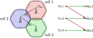
Figure 1: Each base station serves the users located in its cell. However, its signal can be received over the noise level in some areas of the adjacent cells. For example, the users in cell 2 and 3 receive an interference signal from the base stations in cell 1 and 2, respectively. On the right, the topology of this network is shown. Note that each receiver experiences at most one interference.

This can be seen in Fig. 1 which shows the circular coverage area of three adjacent cells. The area which is allocated to a base station is shown as a hexagon inside a circle. Therefore, there are some areas close to the edges of each cell in which the receiver experiences one interference signal in addition to its own desired signal. As an example, Rx 2 and Rx 3 in Fig. 1 observe an interference from undesired base stations Tx 1 and Tx 2, respectively. Since an interferer which is weaker than noise does not have an impact on the DoF of the network; the corresponding link to that interferer is assumed to be absent in the topology of the network (see the topology of the wireless network in Fig. 1).

III System Model

As it is shown in [6], the capacity of a wired network normalized by the capacity of a single link gives us the degrees of freedom for the corresponding wireless network. For simplicity, and in order to avoid the unnecessary treatment of noise in the wireless network which does not have an impact on the DoF of the network, we study the wired noiseless network. Consider three Tx’s which want to communicate with their desired Rx’s. Tx $i$, $i\in\{1,2,3\}$ wants to send a message $W_{i}$ to Rx $i$. It encodes this message into a length-$n$ sequence $\boldsymbol{X}_{i}=(X_{i}(1),\ldots,X_{i}(n))$ and sends this sequence. The received symbol at Rx ${j}$ in $k$th channel use is given by

$$Y_{j}(k)=\sum_{i=1}^{3}h_{ji}(k)X_{i}(k),\quad\forall j\in\{1,2,3\}$$ (1)

where $X_{i}(k)$ and $h_{ji}(k)$ denote the transmitted symbol by Tx $i$ and the channel coefficient corresponding to the link between Tx $i$ and Rx ${j}$. All symbols are chosen from a Galois Field $\mathbb{GF}$. Moreover, the linear operations are performed over this $\mathbb{GF}$. The capacity of each channel is $\log|\mathbb{GF}|$, where $|\mathbb{GF}|$ represents the cardinality of $\mathbb{GF}$. Therefore, only one symbol can be transmitted over a link per channel use.

In our model, CSIT is restricted only to the topology of the network. Therefore, the only information available to the transmitters is about the presence or absence of links but not about the channel coefficients. However, both the local channel coefficients and the topology of the network are known at the receivers.

Since the channel coefficients change, the topology of the network varies during the transmission. Following the motivation in Fig. 1, the desired channels always exist and each receiver is disturbed by at most one interferer. Therefore, the network has a total of 27 topologies as shown in Fig. 2.

It is worth to note that the receivers have an infinite memory and they start the decoding after receiving a complete sequence $\boldsymbol{Y}_{j}$. Therefore, the order of the occurrence of the states is not important. Let $\mathcal{A}$ be a set of states shown in Fig. 2 and $\boldsymbol{X}_{i,\mathcal{A}}$ be the sequence of transmitted symbols by Tx $i$ in all states in $\mathcal{A}$. Assuming a length-$n$ sequence $\boldsymbol{X}$, the length of $\boldsymbol{X}_{i,\mathcal{A}}$ is $n\lambda_{\mathcal{A}}$, where $\lambda_{\mathcal{A}}$ denotes the sum of the probabilities of the states in $\mathcal{A}$.

The goal of this work is to study the DoF gain obtained by jointly encoding across the alternating topologies, when all states occur with the same probability.

Figure 2: All possible states for the three users interference channel, when each receiver observes at most one interferer. The desired links are always present.

IV Main Result

The following theorem provides the main result of this work.

Theorem 1.

The three user interference channel with alternating connectivity and equiprobable states with at most one interferer per receiver has DoF=$2+1/9$.

Proof.

We establish Theorem 1 by showing that the sum capacity of the corresponding wired network is $(2+\frac{1}{9})\log|\mathbb{GF}|$. In order to do this, we need to find an optimal achievability scheme. The optimality of the scheme is shown by comparing it with a tight upper bound of the sum capacity. We start by proposing an achievability scheme leading to a DoF lower bound denoted DoF.

Achievability:

The achievability is based on the joint encoding over the sates [7]. To this end, consider states $B_{1}$, $C_{1}$, $D_{1}$, and $H_{1}$ in Fig. 2. It can be seen that all interference links in states $B_{1}$, $C_{1}$, and $D_{1}$ are present in state $H_{1}$. Therefore, we can utilize state $H_{1}$ to resolve the interferences in these states. As it is shown in Fig. 3, the symbols $b_{1}$, $c_{2}$, and $d_{3}$ cannot be decoded at the desired receivers in states $B_{1}$, $C_{1}$, and $D_{1}$. However, by using the state $H_{1}$, the transmitters provide the symbols which cause interference in states $B_{1}$, $C_{1}$, and $D_{1}$ to the receivers. Therefore, in total $9$ symbols are decoded correctly at the desired receivers by combining these four states. Similarly, the same joint encoding scheme can be used for $B_{2}$, $C_{2}$, $D_{2}$, and $H_{2}$ due to symmetry. The remaining states are encoded individually. In all these states except in state $A$, we achieve DoF=2 by choosing two active transmitters. For instance, in state $I_{1}$, DoF=2 is achievable when Tx 2 and Tx 3 send while Tx 1 is silent. Overall, the following DoF is achievable

$$\text{\text@underline{DoF}}=\begin{cases}9/4&\quad\text{for }B_{1}\cup C_{1}\cup D_{1}\cup H_{1}\\ 9/4&\quad\text{for }B_{2}\cup C_{2}\cup D_{2}\cup H_{2}\\ 3&\quad\text{for }A\\ 2&\quad\text{in all remaining 18 states }\end{cases}$$

Since, all states occur with equal probability, we can transmit 57 symbols reliably in 27 channel uses in average. Since every symbol is chosen from $\mathbb{GF}$ with the entropy $\log|\mathbb{GF}|$, the achievable sum rate is

$$R_{\Sigma}\leq\left(2+\frac{1}{9}\right)\log|\mathbb{GF}|.$$ (2)

Figure 3: By combining these four states, we can recover $9$ symbols. However, by considering them separately, we cannot exceed $15/2$ symbols.

Upper bound:

We establish the upper bound as follows

$$nR_{\Sigma}= \sum_{i=1}^{3}H(W_{i})$$

$$= \sum_{i=1}^{3}H(W_{i})+H(W_{i}|\boldsymbol{Y}_{i})-H(W_{i}|\boldsymbol{Y}_{i})$$

$$\overset{(a)}{\leq} \sum_{i=1}^{3}I(W_{i};\boldsymbol{Y}_{i})+3n\epsilon_{n},$$ (3)

where ($a$) follows from Fano’s inequality and $\epsilon_{n}\rightarrow 0$ when $n\rightarrow\infty$. By multiplying the inequality in (3) by 2, every mutual information appears twice which corresponds to creating (virtually) three additional receivers. In the next step, we give side information to the actual receivers. The side information equals to the undesired messages at those receivers. Therefore, we write

$$2nR_{\Sigma}\leq I(W_{1};\boldsymbol{Y}_{1},W_{2},W_{3})+I(W_{2};\boldsymbol{Y}_{2},W_{1},W_{3})$$ (4)

$$+I(W_{3};\boldsymbol{Y}_{3},W_{1},W_{2})+\sum_{i=1}^{3}I(W_{i};\boldsymbol{Y}_{i})+6n\epsilon_{n}.$$

By using the chain rule and since the messages of three transmitters are independent from each other, we write

$$2nR_{\Sigma} \leq I(W_{1};\boldsymbol{Y}_{1}|W_{2},W_{3})+I(W_{2};\boldsymbol{Y}_{2}|W_{1},W_{3})$$

$$\quad+I(W_{3};\boldsymbol{Y}_{3}|W_{1},W_{2})+\sum_{i=1}^{3}I(W_{i};\boldsymbol{Y}_{i})+6n\epsilon_{n}.$$ (5)

By expressing the mutual information as entropy terms, (5) is restated as

$$2nR_{\Sigma} \leq H(\boldsymbol{Y}_{1}|W_{2},W_{3})-H(\boldsymbol{Y}_{1}|W_{2},W_{3},W_{1})$$

$$\quad+H(\boldsymbol{Y}_{2}|W_{1},W_{3})-H(\boldsymbol{Y}_{2}|W_{1},W_{3},W_{2})$$

$$\quad+H(\boldsymbol{Y}_{3}|W_{1},W_{2})-H(\boldsymbol{Y}_{3}|W_{1},W_{2},W_{3})$$

$$\quad+\sum_{i=1}^{3}I(W_{i};\boldsymbol{Y}_{i})+6n\epsilon_{n}.$$ (6)

Note that knowing all messages, $\boldsymbol{Y}_{i}$ can be reconstructed. Therefore, $H(\boldsymbol{Y}_{i}|W_{1},W_{2},W_{3})=0$. The first term in (6) reduces to

$$H(\boldsymbol{Y}_{1}|W_{2},W_{3})=H(\boldsymbol{X}_{1}),$$

as $\boldsymbol{X}_{1}$ is independent of $W_{2}$ and $W_{3}$ and the fact that scaling a discrete random variable by a constant does not influence entropy [8]. Similar treatment applies to $H(\boldsymbol{Y}_{2}|W_{1},W_{3})$ and $H(\boldsymbol{Y}_{3}|W_{1},W_{2})$ in (6). Next, we rewrite (6) as shown in (7) on the top of next page. The parameters $\Delta_{i}$, $\Gamma_{i}$, and $\Theta_{i}$, $i\in\{1,2,3\}$ are defined as follows

$$\Delta_{1} =\{D_{1},F_{1},G_{1},H_{1},I_{1},K_{1},K_{2},D_{3}\}$$

$$\Gamma_{1} =\{B_{2},E_{2},G_{2},H_{2},I_{2},B_{3}\}$$

$$\Theta_{1} =\overline{\{E_{3}\}\cup\Delta_{1}\cup\Gamma_{1}}$$

$$\Delta_{2} =\{B_{1},E_{1},G_{1},H_{1},I_{1},J_{1},I_{2},B_{3}\}$$

$$\Gamma_{2} =\{C_{2},E_{2},F_{2},H_{2},J_{2},C_{3}\}$$

$$\Theta_{2} =\overline{\{F_{3}\}\cup\Delta_{2}\cup\Gamma_{2}}$$

$$\Delta_{3} =\{C_{1},E_{1},F_{1},H_{1},J_{1},K_{1},J_{2},C_{3}\}$$

$$\Gamma_{3} =\{D_{2},F_{2},G_{2},H_{2},K_{2},D_{3}\}$$

$$\Theta_{3} =\overline{\{G_{3}\}\cup\Delta_{3}\cup\Gamma_{3}}.$$

The notation $\overline{\mathcal{A}}$ denotes the complement set of $\mathcal{A}$.

$$2nR_{\Sigma}\leq H(\boldsymbol{X}_{1,E_{3}},\boldsymbol{X}_{1,\Delta_{1}},\boldsymbol{X}_{1,\Gamma_{1}},\boldsymbol{X}_{1,\Theta_{1}})+H(\boldsymbol{X}_{2,F_{3}},\boldsymbol{X}_{2,\Delta_{2}},\boldsymbol{X}_{2,\Gamma_{2}},\boldsymbol{X}_{2,\Theta_{2}})+H(\boldsymbol{X}_{3,G_{3}},\boldsymbol{X}_{3,\Delta_{3}},\boldsymbol{X}_{3,\Gamma_{3}},\boldsymbol{X}_{3,\Theta_{3}})$$

$$+H(\boldsymbol{X}_{1,E_{3}},\boldsymbol{Y}_{1,\overline{E_{3}}})-H(\boldsymbol{X}_{2,F_{3}},\boldsymbol{X}_{2,\Delta_{2}},\boldsymbol{X}_{3,G_{3}},\boldsymbol{X}_{3,\Gamma_{3}},\boldsymbol{X}_{3,K_{1}},\boldsymbol{X}_{3,J_{2}})$$

$$+H(\boldsymbol{X}_{2,F_{3}},\boldsymbol{Y}_{2,\overline{F_{3}}})-H(\boldsymbol{X}_{3,G_{3}},\boldsymbol{X}_{3,\Delta_{3}},\boldsymbol{X}_{1,E_{3}},\boldsymbol{X}_{1,\Gamma_{1}},\boldsymbol{X}_{1,I_{1}},\boldsymbol{X}_{1,K_{2}})$$

$$+H(\boldsymbol{X}_{3,G_{3}},\boldsymbol{Y}_{3,\overline{G_{3}}})-H(\boldsymbol{X}_{1,E_{3}},\boldsymbol{X}_{1,\Delta_{1}},\boldsymbol{X}_{2,F_{3}},\boldsymbol{X}_{2,\Gamma_{2}},\boldsymbol{X}_{2,J_{1}},\boldsymbol{X}_{2,I_{2}})+6n\epsilon_{n}$$ (7)

 

$$H(\boldsymbol{X}_{1,E_{3}},\boldsymbol{X}_{1,\Delta_{1}},\boldsymbol{X}_{1,\Gamma_{1}},\boldsymbol{X}_{1,\Theta_{1}}) \leq H(\boldsymbol{X}_{1,E_{3}})+H(\boldsymbol{X}_{1,\Delta_{1}}|\boldsymbol{X}_{1,E_{3}})+H(\boldsymbol{X}_{1,\Gamma_{1}}|\boldsymbol{X}_{1,E_{3}})+H(\boldsymbol{X}_{1,\Theta_{1}})$$ (8)

$$H(\boldsymbol{X}_{2,F_{3}},\boldsymbol{X}_{2,\Delta_{2}},\boldsymbol{X}_{2,\Gamma_{2}},\boldsymbol{X}_{2,\Theta_{2}}) \leq H(\boldsymbol{X}_{2,F_{3}})+H(\boldsymbol{X}_{2,\Delta_{2}}|\boldsymbol{X}_{2,F_{3}})+H(\boldsymbol{X}_{2,\Gamma_{2}}|\boldsymbol{X}_{2,F_{3}})+H(\boldsymbol{X}_{2,\Theta_{2}})$$ (9)

$$H(\boldsymbol{X}_{3,G_{3}},\boldsymbol{X}_{3,\Delta_{3}},\boldsymbol{X}_{3,\Gamma_{3}},\boldsymbol{X}_{3,\Theta_{3}}) \leq H(\boldsymbol{X}_{3,G_{3}})+H(\boldsymbol{X}_{3,\Delta_{3}}|\boldsymbol{X}_{3,G_{3}})+H(\boldsymbol{X}_{3,\Gamma_{3}}|\boldsymbol{X}_{3,G_{3}})+H(\boldsymbol{X}_{3,\Theta_{3}})$$ (10)

$$H(\boldsymbol{X}_{1,E_{3}},\boldsymbol{Y}_{1,\overline{E_{3}}}) \leq H(\boldsymbol{X}_{1,E_{3}})+H(\boldsymbol{Y}_{1,\overline{E_{3}}}|\boldsymbol{X}_{1,E_{3}})$$ (11)

$$H(\boldsymbol{X}_{2,F_{3}},\boldsymbol{X}_{2,\Delta_{2}},\boldsymbol{X}_{3,G_{3}},\boldsymbol{X}_{3,\Gamma_{3}},\boldsymbol{X}_{3,K_{1}},\boldsymbol{X}_{3,J_{2}}) \geq H(\boldsymbol{X}_{2,F_{3}})+H(\boldsymbol{X}_{2,\Delta_{2}}|\boldsymbol{X}_{2,F_{3}})+H(\boldsymbol{X}_{3,G_{3}})+H(\boldsymbol{X}_{3,\Gamma_{3}}|\boldsymbol{X}_{3,G_{3}})$$ (12)

$$H(\boldsymbol{X}_{2,F_{3}},\boldsymbol{Y}_{2,\overline{F_{3}}}) \leq H(\boldsymbol{X}_{2,F_{3}})+H(\boldsymbol{Y}_{2,\overline{F_{3}}}|\boldsymbol{X}_{2,F_{3}})$$ (13)

$$H(\boldsymbol{X}_{3,G_{3}},\boldsymbol{X}_{3,\Delta_{3}},\boldsymbol{X}_{1,E_{3}},\boldsymbol{X}_{1,\Gamma_{1}},\boldsymbol{X}_{1,I_{1}},\boldsymbol{X}_{1,K_{2}}) \geq H(\boldsymbol{X}_{3,G_{3}})+H(\boldsymbol{X}_{3,\Delta_{3}}|\boldsymbol{X}_{3,G_{3}})+H(\boldsymbol{X}_{1,E_{3}})+H(\boldsymbol{X}_{1,\Gamma_{1}}|\boldsymbol{X}_{1,E_{3}})$$ (14)

$$H(\boldsymbol{X}_{3,G_{3}},\boldsymbol{Y}_{3,\overline{G_{3}}}) \leq H(\boldsymbol{X}_{3,G_{3}})+H(\boldsymbol{Y}_{3,\overline{G_{3}}}|\boldsymbol{X}_{3,G_{3}})$$ (15)

$$H(\boldsymbol{X}_{1,E_{3}},\boldsymbol{X}_{1,\Delta_{1}},\boldsymbol{X}_{2,F_{3}},\boldsymbol{X}_{2,\Gamma_{2}},\boldsymbol{X}_{2,J_{1}},\boldsymbol{X}_{2,I_{2}}) \geq H(\boldsymbol{X}_{1,E_{3}})+H(\boldsymbol{X}_{1,\Delta_{1}}|\boldsymbol{X}_{1,E_{3}})+H(\boldsymbol{X}_{2,F_{3}})+H(\boldsymbol{X}_{2,\Gamma_{2}}|\boldsymbol{X}_{2,F_{3}})$$ (16)

 

By using the chain rule, together with the facts that conditioning does not increase entropy, and that the messages of the users are independent of each other, the individual terms in (7) can be rewritten as in (8)-(16) on the top of next page. We can see that by substituting (8)-(16) into (7) many terms will cancel out and we can rewrite (7) as

$$2nR_{\Sigma}\leq \sum_{i=1}^{3}H(\boldsymbol{X}_{i,\Theta_{i}})+H(\boldsymbol{Y}_{1,\overline{E_{3}}}|\boldsymbol{X}_{1,E_{3}})$$ (17)

$$+H(\boldsymbol{Y}_{2,\overline{F_{3}}}|\boldsymbol{X}_{2,F_{3}})+H(\boldsymbol{Y}_{3,\overline{G_{3}}}|\boldsymbol{X}_{3,G_{3}})+6n\epsilon_{n}.$$

The inequality (17) can be further upper bounded by

$$2nR_{\Sigma}\leq \log|\mathbb{GF}|[n\lambda_{\Theta_{1}}+n\lambda_{\Theta_{2}}+n\lambda_{\Theta_{3}}+n(1-\lambda_{E_{3}})$$

$$+n(1-\lambda_{F_{3}})+n(1-\lambda_{G_{3}})]+6n\epsilon_{n},$$ (18)

where we used the chain rule, the fact that conditioning does not increase the entropy, and that the entropy of discrete random variable in $\mathbb{GF}$ is upper bounded by $\log|\mathbb{GF}|$ [8].

Since the set $\Theta_{i}$ consists of 12 states, $\lambda_{\Theta_{i}}=\frac{12}{27}$ if all states are equiprobable. Next, we divide the inequality in (18) by $2n$, and let $n\rightarrow\infty$ to obtain

$$R_{\Sigma}\leq \left(2+\frac{1}{9}\right)\log|\mathbb{GF}|.$$ (19)

This agrees with the lower bound in (2). Normalizing the result by $\log|\mathbb{GF}|$, we get the DoF for the wireless case which proves Theorem 1. ∎

We observe from Theorem 1 that no joint processing is necessary for $\overline{\{B_{1},C_{1},D_{1},H_{1},B_{2},C_{2},D_{2},H_{2}\}}$. However, for $\{B_{1},C_{1},D_{1},H_{1},B_{2},C_{2},D_{2},H_{2}\}$, we need joint encoding to achieve the optimal DoF. The alternative approach would be to treat these states separately as well. This would result in a DoF=$3/2$ and DoF=$2$ for the states $\{H_{1},H_{2}\}$ (as shown in [9]) and $\{B_{1},C_{1},D_{1},B_{2},C_{2},D_{2}\}$ (as shown in [10]), respectively. Therefore, the overall DoF=2 is optimal for separate encoding while by using joint encoding across the alternating topologies $2+1/9$ is the optimal achievable DoF.

V Conclusion

We studied the DoF of the three users interference channel with an alternating connectivity with only topological knowledge at the transmitters. To do this, we proposed a new joint encoding across the alternating topologies. Moreover, a new genie aided upper bound is established to verify the optimality of the joint encoding scheme. The upper bound is tight for the equiprobable case. As future work, the non-equiprobable case will be addressed. However, this extension is non-trivial due to the increase in the number of possible combination of states.

References

• [1] M. Maddah-Ali and D. Tse, “Completely stale transmitter channel state information is still very useful,” in 48th Allerton Conf. on CCC, 2010, pp. 1188–1195.
• [2] H. Maleki, S. A. Jafar, and S. Shamai, “Retrospective Interference Alignment over Interference Networks,” IEEE Journal of Selected Topics in Signal Processing.
• [3] T. Gou and S. A. Jafar, “Optimal use of current and outdated channel state information – degrees of freedom of the MISO BC with mixed CSIT,” IEEE Comm. Letters, vol. 16, no. 7, pp. 1084–1087, July 2012.
• [4] M. Kobayashi, S. Yang, D. Gesbert, and X. Yi, “On the degrees of freedom of time correlated MISO broadcast channel with delayed CSIT,” in IEEE ISIT, 2012, pp. 2501–2505.
• [5] R. Tandon, S. Jafar, S. Shamai Shitz, and H. Poor, “On the synergistic benefits of alternating CSIT for the MISO broadcast channel,” IEEE Trans. on IT, July 2013.
• [6] S. A. Jafar, “Topological interference management through index coding,” Jan. 2013. [Online]. Available: http://arxiv.org/pdf/1301.3106.pdf
• [7] H. Sun, C. Geng, and S. A. Jafar, “Topological interference management with alternating connectivity,” Feb. 2013. [Online]. Available: http://arxiv.org/abs/1302.4020
• [8] T. M. Cover and J. A. Thomas, Elements of Information Theory.   John Wiley & Sons, August 1991.
• [9] L. Zhou and W. Yu, “On the symmetric capacity of the K-user symmetric cyclic Gaussian interference channel,” in CISS, Princeton, NJ, 2010.
• [10] R. H. Etkin, D. N. C. Tse, and H. Wang, “Gaussian interference channel capacity to within one bit,” IEEE Trans. on IT, vol. 54, no. 12, pp. 5534–5562, Dec. 2008.