Stationary Wigner Equation with Inflow Boundary Conditions: Will a Symmetric Potential Yield a Symmetric Solution?

Abstract

Based on the well-posedness of the stationary Wigner equation with inflow boundary conditions given in [1], we prove without any additional prerequisite conditions that the solution of the Wigner equation with symmetric potential and inflow boundary conditions will be symmetric. This improve the result in [8] which depends on the convergence of solution formulated in the Neumann series. By numerical studies, we present the convergence of the numerical solution to the symmetric profile for three different numerical schemes. This implies that the upwind schemes can also yield a symmetric numerical solution, on the contrary to the argument given in [8].

Keywords: Wigner equation; Inflow boundary conditions; Well-posedness.

1 Introduction

The stationary dimensionless Wigner equation can be written as [9]

$$v\dfrac{\partial{f(x,v)}}{\partial{x}}+\int\,\mathrm{d}v^{\prime}V_{w}(x,v-v^{\prime})f(x,v^{\prime})=0,$$ (1.1)

where the Wigner potential $V_{w}(x,v)$ is related to the potential $V(x)$ through

$$V_{w}(x,v)=\frac{\mathrm{i}}{2\pi}\int\,\mathrm{d}y~{}\mathrm{e}^{-\mathrm{i}vy}\left[V(x+y/2)-V(x-y/2)\right].$$ (1.2)

We are considering the inflow boundary conditions proposed in [3] and analyzed in [1, 8], which specifies the inflow electron distribution function $f(-l/2,v)$, $v>0$ at the left contact ($x=-l/2$) and $f(l/2,v)$, $v<0$ at the right contact ($x=l/2$). In [8], the Wigner equation with a symmetric potential ($V(-x)=V(x)$) is considered. It was declared in [8] that (1.1) with a symmetric potential gives always a Wigner function symmetric in the spatial coordinate: $f(x,v)=f(-x,v)$, no matter what profile of the injected carrier distribution is. Actually, it is not true for all the symmetric potential functions. For example, when $V(x)=1-x^{2}/2$, the Wigner equation will reduce to its classical counterpart, the Boltzmann equation (the Liouville equation)

$$v\dfrac{\partial{f(x,v)}}{\partial{x}}+x\dfrac{\partial{f(x,v)}}{\partial{v}}=0.$$ (1.3)

One may figure out the solution of (1.3) by examining rolling balls to a hill with a shape $V(x)=1-x^{2}/2$. When one roll a ball with the initial kinetic energy less than the height of $V(x)$ (which is $1$ at $x=0$), it is impossible to find the ball on the right hand side. This implies that a symmetric potential can not assure a symmetric distribution. Let us put forward a question:

For which class of symmetric potential the equation (1.1) always has a symmetric solution for any inflow boundary conditions?

In this paper, we answer this question partly by proving that for a symmetric and periodic potential with a period $l$, the Wigner equation (1.1) with inflow boundary conditions has one and only one symmetric solution. The proof hereafter is based on the elegant approach of the well-posedness of the stationary Wigner equation with inflow boundary conditions in [1]. The proof in [1] is given only for the discrete velocity version of the Wigner equation providing that $0$ is excluded from the discrete velocity points adopted. What under our consideration is the continuous version of the Wigner equation (1.1) with the periodic condition of the potential function. By the periodicity of $V(x)$, we first simplify the Wigner equation to a form equivalent to its discrete velocity version. Then we are able to make use of the well-posedness theorem in [1] to prove the symmetric property.

In [8], a center finite-difference method was proposed to provide a symmetric solution. It was declared therein that the numerical solution will give an asymmetric solution in case of the first-order upwind finite difference scheme used. This indicates that the first-order upwind finite difference scheme will not converge to the exact solution at all, which is predicted theoretically to be symmetric in $x$. It argued that the strange numerical behavior is due to that the center scheme is more physical than the upwind scheme. On doubt of this point of view, we revisit the numerical example in [8] using three different numerical schemes, including the two schemes used in [8] and a second-order upwind finite difference schemes. Our numerical results demonstrate that the first-order finite difference method and the second-order upwind finite difference scheme can also give symmetric solutions as long as the gird size is small enough. Moreover, the symmetry of the numerical solution can be quantitatively bounded by the accuracy of the numerical solution. Thus it is found out that whether the numerical solution is symmetric is not only related to numerical scheme, but also related to the numerical accuracy.

The remain part of this paper is arranged as below: in Section 2, we prove the symmetry of the solution of (1.1) with symmetric potential and in Section 3, the numerical study of the example in [8] is presented.

2 Symmetry of Solution of (1.1) with Symmetric Potential

In general, the well-posedness of the boundary value problem (BVP) for the stationary Wigner equation

$$v\dfrac{\partial{f(x,v)}}{\partial{x}}+\int\,\mathrm{d}v^{\prime}V_{w}(x,v-v^{\prime})f(x,v^{\prime})=0,x\in(-l/2,l/2),v\in\mathbb{R},$$ (2.1)

with the inflow boundary conditions

$$f(-l/2,v)=f_{b}(v),\text{ for }v>0;\quad f(+l/2,v)=f_{b}(v),\text{ for }v<0,$$ (2.2)

is an open problem [1].

At first, we expand the potential $V(x)$ into a Fourier series. The Fourier series is uniformly converged to $V(x)$ under mild conditions, e.g., if $V(x)$ is periodic, continuous, and its derivative $V^{\prime}(x)$ is piecewise continuous. Particularly, if $V(x)$ is symmetric with respect to $y$-axis, i.e. it is an even function, we can expand it to cosine series. In this paper, we consider a special case in which the potential function $V(x)$ defining $V_{w}$ through (1.2) is a periodic ($V(x+l)=V(x)$), even function with an absolutely convergent Fourier series, i.e.,

$$V(x)=a_{0}+\sum_{n=1}^{\infty}a_{n}\,\cos(2n\kappa x),$$ (2.3)

where $\kappa=\frac{\pi}{l}$ and $\sum_{n=0}^{\infty}|a_{n}|$ is finite. Several sufficient conditions for $V(x)$ to have an absolutely convergent Fourier series are given in [5], e.g., if $V(x)$ is absolutely continuous in $[-l/2,l/2]$ and $V^{\prime}(x)\in L^{2}[-l/2,l/2]$, then $V(x)$ has an absolutely convergent Fourier series. We will prove that the boundary value problem (BVP) (2.1), (2.2) is well-posed, and its solution is symmetric, i.e., $f(x,v)=f(-x,v)$, $v\neq 0$, no matter what profile of the injected carrier distribution is, providing that $V(x)$ has an expansion (2.3). For $V(x)$ with an expansion in (2.3), a direct calculation of (1.2) yields

$$V_{w}(x,v)=\sum_{n=1}^{\infty}a_{n}\sin(2n\kappa x)\left(\delta(v+n\kappa)-\delta(v-n\kappa)\right).$$ (2.4)

Thus, plugging (2.4) into the Wigner equation (2.1), we reformulate the stationary dimensionless Wigner equation as

$$v\frac{\partial f(x,v)}{\partial x}+\sum_{n=1}^{\infty}a_{n}\sin(2n\kappa x)\left(f(x,v+n\kappa)-f(x,v-n\kappa)\right)=0,$$ (2.5)

where $x\in(-l/2,l/2)$ and $v\in\mathbb{R}$.

Observing (2.5), one can see that $v$ can be viewed as a parameter, and (2.5) can be regarded as a set of ordinary differential equations, and $f(x,v)$ only couples with $f(v+n\kappa),n\in\mathbb{Z}$. The BVP (2.5) with inflow boundary conditions (2.2) can be decoupled into independent ordinary differential systems indexed by $s\in(0,\kappa)$

$$v_{i}^{s}\dfrac{\,\mathrm{d}{f(x,v_{i}^{s})}}{\,\mathrm{d}{x}}+\sum_{n=1}^{\infty}a_{n}\sin(2n\kappa x)\left(f(x,v_{i+n}^{s})-f(x,v_{i-n}^{s})\right)=0,\quad x\in(-l/2,l/2),i\in\mathbb{Z},$$ (2.6)

under the inflow boundary conditions

$$f(-l/2,v_{i}^{s})=f_{b}(v_{i}),\text{ for }i\geqslant 0;\quad f(l/2,v_{i}^{s})=f_{b}(v_{i}),\text{ for }i<0,\$$ (2.7)

where $v_{i}^{s}=i\kappa+s$. Notice that we have to neglect the case $s=0$ until now.

Remark 1.

If $s=0$, (2.6) becomes an algebraic-differential system and its property is quite different, and it will bring difficulty to the theoretical analysis [1]. And to the authors’ best knowledge, $0$ is also excluded from the sampling velocity set in all numerical simulation papers e.g., [3, 4].

Let $f^{s}_{i}(x)$ denote $f(x,v_{i}^{s})$ and the vector $\mathbf{f}(x)=\{f^{s}_{i}(x),i\in\mathbb{Z}\}$ denote the discrete velocity Wigner function on the discrete velocity set $\mathbf{v}^{s}=\{v_{i}^{s}:=i\kappa+s,i\in\mathbb{Z}\}$. The discrete velocity $v_{i}^{s}\in\mathbb{R}$ are strictly increasing, i.e., $v_{i}^{s}<v^{s}_{i+1}$. Considering the singularity of the equation when $v=0$, we have excluded $0$ from $\mathbf{v}^{s}$ by setting $s\neq 0$. Henceforth, we omit the superscript ^s of $f^{s}_{i}(x)$, $\mathbf{f}^{s}$, $\mathbf{v}^{s}$ and $v_{i}^{s}$ when no confusion happens.

Then we rewrite the stationary Wigner equation (2.6) to be its discrete counterpart as

$$\boldsymbol{T}\mathbf{f}_{x}-\boldsymbol{A}(x)\mathbf{f}=0,\,\,-l/2<x<l/2,$$ (2.8)

subject to the inflow boundary conditions (2.7) rewritten into

$$f_{i}(-l/2)=f_{b}(v_{i}),\text{ for }i\geqslant 0,\quad f_{i}(l/2)=f_{b}(v_{i}),\text{ for }i<0,$$ (2.9)

with a given sequence $\mathbf{f}_{b}=\{f_{b}(v_{i}),i\in\mathbb{Z}\}$. Here,

$$\boldsymbol{T}=\text{diag}\{\cdots,v_{-2},v_{-1},v_{0},v_{1},v_{2}\cdots\}$$

and

$$\boldsymbol{A}(x)=\left(\begin{array}[]{ccccccc}&\ddots&&&&&\\ \cdots&a_{1}\sin(2\kappa x)&0&-a_{1}\sin(2\kappa x)&-a_{2}\sin(4\kappa x)&-a_{3}\sin(6\kappa x)&\cdots\\ \cdots&a_{2}\sin(4\kappa x)&a_{1}\sin(2\kappa x)&0&-a_{1}\sin(2\kappa x)&-a_{2}\sin(4\kappa x)&\cdots\\ \cdots&a_{3}\sin(6\kappa x)&a_{2}\sin(2\kappa x)&a_{1}\sin(2\kappa x)&0&-a_{1}\sin(2\kappa x)&\cdots\\ &&&&&\ddots&\end{array}\right)$$

which is a skew-symmetric matrix.

Let the linear space $H_{w}=l^{2}(\mathbb{Z};w_{i})$ equipped with the canonical weighted $l^{2}$ norm

$$\|\mathbf{f}\|_{H_{w}}=\left(\sum_{i\in\mathbb{Z}}w_{i}|f_{i}|^{2}\right)^{1/2},$$

where $w_{i}=|w(v_{i})|$ and $w(v)$ be a weight function. Particularly, if $w(v)=v$, the norm of $H_{v}$ is

$$\|\mathbf{f}\|_{H_{v}}=\left(\sum_{i\in\mathbb{Z}}|v_{i}||f_{i}|^{2}\right)^{1/2},$$

and if $w(v)=1$, the norm of $H_{1}$ is

$$\|\mathbf{f}\|_{H_{1}}=\left(\sum_{i\in\mathbb{Z}}|f_{i}|^{2}\right)^{1/2}.$$

We let $H=H_{1}$ and $B(H)$ to be the bounded linear operator on $H$. We have the following

Lemma 1.

If the Fourier coefficients of $V(x)$, $\{a_{n}\}_{n=0}^{\infty}\in l^{1}$, then $\boldsymbol{A}(x)\in B(H)$.

Proof.

Observing

$$(\boldsymbol{A}(x)\mathbf{f}(x))_{k}=\sum_{i=-\infty}^{\infty}a_{|k-i|}\sin(2(k-i)\kappa x)f_{i}(x),$$

one can find that $\boldsymbol{A}(x)\mathbf{f}(x)$ is the discrete convolution i.e.,

$$\boldsymbol{A}(x)\mathbf{f}(x)=\mathbf{v}_{d}(x)\ast\mathbf{f}(x),$$

where $\mathbf{V}_{d}(x)=\{a_{|i|}\sin(2i\kappa x),i\in\mathbb{Z}\}$. We can apply the Young’s inequality to the discrete convolution

$$\boldsymbol{A}(x)\mathbf{f}(x)=\mathbf{V}_{d}(x)\ast\mathbf{f}(x)$$

to have

$$\|\boldsymbol{A}(x)\mathbf{f}(x)\|_{2}=\|\mathbf{V}_{d}(x)\ast\mathbf{f}(x)\|_{2}\leqslant\|\mathbf{V}_{d}(x)\|_{1}\|\mathbf{f}(x)\|_{2}.$$

On the other hand, we have

$$\|\mathbf{V}_{d}\|_{1}=\sum_{i=-\infty}^{\infty}|a_{|i|}\sin(2i\kappa x)|\leqslant 2\sum_{n=1}^{\infty}|a_{n}|\leqslant 2\|\{a_{n}\}_{n=0}^{\infty}\|_{l^{1}}<\infty.$$

Thus by noting that the $H$-norm is the same as the $l^{2}$-norm, we have

$$\|\mathbf{A}(x)\mathbf{f}(x)\|_{H}\leqslant 2\|\{a_{n}\}_{0}^{\infty}\|\|\mathbf{f}\|_{H},$$

which gives the conclusion $\mathbf{A}(x)\in B(H)$ and $\|\mathbf{A}(x)\|\leq 2\|\{a_{n}\}_{0}^{\infty}\|$. ∎

The proof of the well-posedness of the discrete velocity problem has been given in [1], and here we present the conclusion below.

Lemma 2.

(Theorem 3.3 in [1]) Assume $\mathbf{f}_{b}=(\mathbf{f}_{b}^{+},\mathbf{f}_{b}^{-})\in H_{v}$, and let $\boldsymbol{A}(x)\in B(H)$ be skew-symmetric for all $x\in[-l/2,l/2]$. Then one has:

(a) If $\boldsymbol{A}\in L^{1}((-l/2,l/2),B(H))$, the BVP (2.8) and (2.9) has a unique mild solution $\mathbf{f}(x)\in W^{1,1}((-l/2,l/2),H_{v})$. Also, $\boldsymbol{T}\mathbf{f}_{x}\in L^{1}\left((-l/2,l/2),H\right)$;

(b) If $\boldsymbol{A}(x)$ is strongly continuous in x on $[-l/2,l/2]$ and uniformly bounded in the norm of $B(H)$ on $[-l/2,l/2]$, then the solution from (a) is classical, i.e., $\mathbf{f}\in C^{1}([-l/2,l/2],H_{v})$. Also, $\boldsymbol{T}\mathbf{f}_{x}\in C([-l/2,l/2],H)$.

Now we are ready to have the following theorem.

Theorem 1.

Assume $V(x)$ is a periodic, even function with an absolutely convergent Fourier series, i.e., $\{a_{n}\}_{n=0}^{\infty}\in l^{1}$. For $\forall s\in(0,\kappa)$, let $\mathbf{f}_{b}=(\mathbf{f}_{b}^{+},\mathbf{f}_{b}^{-})\in H_{v}$ defined by (2.9) on $\mathbf{v}^{s}$. Then the BVP (2.8), (2.9) has a unique solution $\mathbf{f}(x)$, and for the discrete velocity Wigner function on the discrete velocity set $\mathbf{v}^{s}$, $\mathbf{f}(x)$ is a mild solution in $W^{1,1}((-l/2,l/2),H_{v})$.

Proof.

It is clear that $\forall s\in(0,\kappa)$, the corresponding discrete velocity Wigner function $\mathbf{f}(x)$ satisfies the BVP (2.8) and (2.9). By Lemma 1, $A(x)\in B(H)$ and by the assumption, $\mathbf{f}_{b}=(\mathbf{f}_{b}^{+},\mathbf{f}_{b}^{-})\in H_{v}$, thus the requirement of Lemma 2 is fulfilled. Applying Lemma 2, we have that $\mathbf{f}(x)\in W^{1,1}((-l/2,l/2),H_{v})$. This ends the proof. ∎

Based on the well-posedness of the above Wigner equation, the solution of the BVP (2.8) and (2.9) satisfies the following initial value problem (IVP)

$$\dfrac{\,\mathrm{d}{\mathbf{f}(x)}}{\,\mathrm{d}{x}}=T^{-1}\boldsymbol{A}(x)\mathbf{f}(x),\quad x\in(-l/2,l/2),$$ (2.10)

with $\mathbf{f}(x)$ at $x=x_{1}$ is a given vector. One can define a propagator $\mathcal{T}_{[x_{1},x_{2}]}$ via the solution of the IVP (2.10) [7], i.e.,

$$\mathbf{f}(x_{2})=\mathcal{T}_{[x_{1},x_{2}]}\mathbf{f}(x_{1}).$$

Clearly, the operator $\mathcal{T}_{[x_{1},x_{2}]}$ is invertible and

$$\mathcal{T}_{[x_{1},x_{2}]}^{-1}=\mathcal{T}_{[x_{2},x_{1}]}.$$

More properties of $\mathcal{T}_{[x_{1},x_{2}]}$ can be found in [7].

Moreover, if the potential is symmetric, i.e., $V(x)=V(-x)$, we have the following lemma.

Lemma 3.

If $V(x)$ is a periodic, even function with an absolutely convergent Fourier series, i.e., $\{a_{n}\}_{n=0}^{\infty}\in l^{1}$, then $\mathcal{T}_{[0,x]}=\mathcal{T}_{[0,-x]}$, $\forall x\in(-l/2,l/2)$.

Proof.

The IVP (2.10) can be recast into an integral equation

$$\mathbf{f}(x)=\mathbf{f}(x_{1})+\int_{x_{1}}^{x}T^{-1}A(y)\mathbf{f}(y)\,\mathrm{d}y=\mathbf{f}(x_{1})+K_{[x_{1},x_{2}]}\mathbf{f}(x),\quad x\in[x_{1},x_{2}]\text{ or }x\in[x_{2},x_{1}],$$ (2.11)

where $K_{[x_{1},x_{2}]}$ is defined by

$$K_{[x_{1},x_{2}]}\mathbf{f}(x)=\int_{x_{1}}^{x}T^{-1}A(y)\mathbf{f}(y)\,\mathrm{d}y,\text{ for }x\in[x_{1},x_{2}]\text{ or }x\in[x_{2},x_{1}]$$

We have that

$$\|K_{[x_{1},x_{2}]}\mathbf{f}(x)\|_{H,\infty}\leqslant\dfrac{C|x_{1}-x_{2}|}{\min_{i\in\mathbb{Z}}|v_{i}|}\|\mathbf{f}(x)\|_{H,\infty},$$

where the norm of the vector function $\mathbf{g}(x),x\in[x_{1},x_{2}]$ is defined by

$$\|\mathbf{g}(x)\|_{H,\infty}=\text{sup}_{x\in[x_{1},x_{2}]}\|\mathbf{g}(x)\|_{H},$$

$C$ is the twice of the $l^{1}$ norm of the Fourier coefficients of $V(x)$. Noticing that $\min_{j\in\mathbb{Z}}|v_{j}|>0$, we have that

$$\|K_{[x_{1},x_{2}]}\|_{C\left([x_{1},x_{2}],H\right)}<1,$$

if $|x_{1}-x_{2}|<\tilde{\delta}=\min_{j\in\mathbb{Z}}|v_{j}|/C>0$. By applying the Neumann series to (2.11), we have

$$\mathbf{f}(x)=(I-K_{[x_{1},x_{2}]})^{-1}\mathbf{f}^{(0)}(x)=\sum_{n=0}^{\infty}K_{[x_{1},x_{2}]}^{n}\mathbf{f}^{(0)}(x),$$

or

$$\mathbf{f}(x)=\lim_{n\rightarrow\infty}\mathbf{f}^{(n)}(x),$$ (2.12)

where

$$\begin{split}&\mathbf{f}^{(0)}(x)=\mathbf{f}(x_{1}),\quad x\in[x_{1},x_{2}]\text{ or }[x_{2},x_{1}],\\ &\mathbf{f}^{(n+1)}(x)=\mathbf{f}(x_{1})+K_{[x_{1},x_{2}]}\mathbf{f}^{(n)}(x),~{}~{}x\in[x_{1},x_{2}]\text{ or }[x_{2},x_{1}],~{}n=0,1,\cdots.\end{split}$$ (2.13)

The Neumann series converges if $|x_{2}-x_{1}|\leq\delta<\tilde{\delta}$. $V(x)$ is symmetric, i.e., $V(x)=V(-x)$, so we see that $\boldsymbol{A}(-x)=-\boldsymbol{A}(x)$. At the same time, $\mathbf{f}^{(0)}(x),x\in[-\delta,\delta]$ is symmetric (actually $\mathbf{f}^{(0)}(x)=\mathbf{f}(0),x\in[-\delta,\delta]$ is a constant vector function of $x$), we have

$$\begin{array}[]{rcl}K_{[0,-\delta]}\mathbf{f}^{(0)}(x)&=&\displaystyle\int_{0}^{-x}T^{-1}A(y)\mathbf{f}^{(0)}(y)\,\mathrm{d}y\\[11.38109pt] &=&\displaystyle\int_{0}^{x}T^{-1}A(-y)\mathbf{f}^{(0)}(-y)\,\mathrm{d}(-y)\\[11.38109pt] &=&\displaystyle\int_{0}^{x}T^{-1}(-A(y))\mathbf{f}^{(0)}(y)(-\,\mathrm{d}y)\\[11.38109pt] &=&\displaystyle\int_{0}^{x}T^{-1}A(y)\mathbf{f}^{(0)}(y)\,\mathrm{d}y=K_{[0,\delta]}\mathbf{f}^{(0)}(x),\end{array}$$

which imples $\mathbf{f}^{(1)}(-x)=\mathbf{f}^{(1)}(x)$. It is easy to see that we can obtain $\mathbf{f}^{(n)}(-x)=\mathbf{f}^{(n)}(x),n=2,3,\cdots$, thus we have $\mathbf{f}(x)=\mathbf{f}(-x),x\in[-\delta,\delta]$, i.e.,

$$\begin{array}[]{rcl}\mathcal{T}_{[0,-x]}\mathbf{f}(0)&=&\mathbf{f}(-x)=\displaystyle\sum_{n=0}^{\infty}K[0,-\delta]^{n}\mathbf{f}^{(0)}(x)\\ &=&\displaystyle\sum_{n=0}^{\infty}K[0,\delta]^{n}\mathbf{f}^{(0)}(x)=\mathbf{f}(x)=\mathcal{T}_{[0,x]}\mathbf{f}(0),\quad x\in[0,\delta].\end{array}$$

Thus $\mathcal{T}_{[0,x]}=\mathcal{T}_{[0,-x]}$ for $|x|\leqslant\delta$. We have shown that $\mathbf{f}(-x)=\mathbf{f}(x)$ for $x\in[-\delta,\delta]$. We define $\mathbf{f}^{0}(x)=\mathbf{f}(-\delta),x\in[-\delta,-2\delta]$, $\mathbf{f}^{(0)}(x)=\mathbf{f}(\delta),x\in[\delta,2\delta]$, and it is easy to see $\mathbf{f}^{(0)}(-x)=\mathbf{f}^{(0)}(x),x\in[-\delta,-2\delta]\bigcup[\delta,2\delta]$. Then using the same argument, we have for $x\in[-\delta,-2\delta]$,

$$\begin{array}[]{rcl}K_{[-\delta,-2\delta]}\mathbf{f}^{(0)}(x)&=&\displaystyle\int_{-\delta}^{x}T^{-1}A(y)\mathbf{f}^{0}(y)\,\mathrm{d}y\\[11.38109pt] &=&\displaystyle\int_{\delta}^{-x}T^{-1}A(-y)\mathbf{f}^{0}(-y)\,\mathrm{d}(-y)\\[11.38109pt] &=&\displaystyle\int_{\delta}^{-x}T^{-1}(-A(y))\mathbf{f}^{(0)}(y)(-\,\mathrm{d}y)\\[11.38109pt] &=&\displaystyle\int_{\delta}^{-x}T^{-1}A(y)\mathbf{f}^{(0)}(y)\,\mathrm{d}y=K_{[\delta,2\delta]}\mathbf{f}^{(0)}(-x),\end{array}$$

and $K_{[-\delta,-2\delta]}\mathbf{f}^{(n)}(x)=K_{[\delta,2\delta]}\mathbf{f}^{(n)}(-x),\ n=2,3,\cdots,$ thus

$$\begin{array}[]{rcl}\mathbf{f}(x)=\mathcal{T}_{[0,x]}\mathbf{f}(0)=\mathcal{T}_{[0,-x]}\mathbf{f}(0)=\mathbf{f}(-x),~{}\forall x\in[-2\delta,-\delta]\bigcup[\delta,2\delta].\end{array}$$

This implies that the domain valid for $\mathcal{T}_{[0,x]}=\mathcal{T}_{[0,-x]}$ can be continuously extended. We conclude that $\mathcal{T}_{[0,x]}=\mathcal{T}_{[0,-x]}$ for $\forall x\in(-l/2,l/2)$. ∎

By the lemma above, we arrive the following theorem.

Theorem 2.

If $V(x)$ is a periodic, even function with an absolutely convergent Fourier series, the solution of the BVP (2.1), (2.2) satisfies

$$f(x,v)=f(-x,v),\quad\forall v\in\mathbb{R},v\neq n\kappa,n\in\mathbb{Z}$$

for any inflow boundary conditions.

Proof.

Since $v\neq n\kappa,n\in\mathbb{Z}$, there exists $s\in(0,\kappa)$ such that $v\in\mathbf{v}^{s}$. Thus $f(x,v)$ is an entry of $\mathbf{f}(x)$, which is Wigner function values at the discrete velocity set $\mathbf{v}^{s}$. From Lemma 3, we have that the discrete velocity Wigner function on $\mathbf{v}^{s}$ satisfies that

$$\mathbf{f}(x)=\mathcal{T}_{[0,x]}\mathbf{f}(0)=\mathcal{T}_{[0,-x]}\mathbf{f}(0)=\mathbf{f}(-x).$$

Then we have $f(x,v)=f(-x,v)$. ∎

Remark 2.

When $v=0$, the problem may be reduced to an ODE system in the same form as (2.8) and (2.9). The equation at $s=0$ in (2.6) is formally turned into an algebraic constraint as

$$\sum_{n=1}^{\infty}a_{n}\sin(2n\kappa x)\left(f_{n}(x)-f_{-n}(x)\right)=0.$$

It is clear that if $f(x,0)\equiv 0$, the well-posedness of the system is still valid. If $f(x,0)\not\equiv 0$, this algebraic constraint above can not always be fulfiled, thus the existence of the solution is negative. One the other hand, the term involving the derivative in $x$ at $v=0$ may be a $0\times\infty$ form, since the derivative ${\partial f(x,0)}/{\partial x}$ is not bounded by any regularity. This makes the algebraic constraint obtained above by formally dropping the first term is doubtable, which requires further investigation.

3 Numerical Study on Symmetry of Solution

In order to verify the theoretical analysis in Theorem 2, we revisit the example in [8] which considers a particular potential profile $V(x)=V_{0}(1+\cos(2\kappa x))$. The corresponding Wigner potential $V_{w}$ in (2.4) is simply given by

$$V_{w}(x,v)=V_{0}\sin(2\kappa x)\left(\delta(v+\kappa)-\delta(v-\kappa)\right).$$ (3.1)

The boundary conditions are extremely simple, too. A mono-energetic carrier injects only from the left boundary, i.e., we set $f_{b}(v_{i})$ in (2.9) to be

$$f_{b}(v_{i})=\begin{cases}1,&\text{if }i=0,\\ 0,&\text{else},\end{cases}$$ (3.2)

where $v_{i}=(i+1/2)\kappa$ which means $s=\kappa/2$ (the index of the differential system (2.6)).

In this section, we will solve the ordinary differential system (2.8)-(2.9) with $V_{w}$ in (3.1), which reduces to

$$v_{i}\dfrac{\,\mathrm{d}{f_{i}(x)}}{\,\mathrm{d}{x}}=V_{0}\sin(2\kappa x)\left(f_{i+1}(x)-f_{i-1}(x)\right),\quad x\in(-l/2,l/2),i\in\mathbb{Z},$$ (3.3)

under inflow boundary conditions (2.9) with inflow data given in (3.2).

Set the other parameters to be $V_{0}=20$, and $l=1$ which gives $\kappa=\pi/l=\pi$. The kinetic energy is $v_{0}^{2}/2$, which is lower than the height of the potential energy in the middle of the device. If using the classic mechanics (the Liouville equation or the Boltzmann equation), one can not see the carrier in the right part of the device. This implies the solution of the classic mechanics equation will be asymmetric.

In the following part of the section, we will show that the numerical solution of the Wigner equation will be symmetric using three numerical schemes. The first scheme is the first-order upwind finite-difference method [3], and the other two are second-order finite-difference methods. The second scheme is the second-order upwind finite-difference method used in many numerical simulation papers, e.g., [4]. The authors of [8] used the first-order upwind finite-difference method and failed to get a symmetric solution, so they proposed a central finite-difference method based on physical argument, which is adopted as our third scheme.

3.1 Three Finite-Difference Schemes

We implement the finite difference methods on a uniform mesh. The $x$-domain $[-l/2,l/2]$ is discretized with $N_{x}+1$ equally distanced grid points $x_{j}=j\Delta x,j=0,1,\cdots,N_{x}$ where $\Delta x=l/N_{x}$. We have to truncate $i\in\mathbb{Z}$ into a finite set $\{i:M\leqslant i\leq M\}$. $M$ depends on the inflow data and the potential strength $V_{0}$, and in our current example, we set $M=40$, which is found large enough for our numerical example. We denote $f_{i}(x)$ at $x=x_{j}$ by $f_{i,j}$. The first order upwind finite-difference scheme is obtained by approximate $\left.\dfrac{\,\mathrm{d}{f_{i}(x)}}{\,\mathrm{d}{x}}\right|_{x_{j}}$ with

$$\left.\dfrac{\,\mathrm{d}{f_{i}(x)}}{\,\mathrm{d}{x}}\right|_{x_{j}}\approx\begin{cases}\frac{f_{i,j+1}-f_{i,j}}{\Delta x},&\text{if }v_{i}<0,\\ \frac{f_{i,j}-f_{i,j-1}}{\Delta x},&\text{if }v_{i}>0,\\ \end{cases}$$

thus yields the finite difference equations of (3.3) as

$$\left\{\begin{array}[]{ll}v_{i}\dfrac{f_{i,j+1}-f_{i,j}}{\Delta x}=g_{i,j},&v_{i}<0,j=0,1,\cdots,N_{x}-1,\\ v_{i}\dfrac{f_{i,j}-f_{i,j-1}}{\Delta x}=g_{i,j},&v_{i}>0,j=1,2,\cdots,N_{x}.\\ \end{array}\right.$$ (3.4)

where

$$g_{i,j}=V_{0}\sin(2\kappa x_{j})(f_{i-1,j}-f_{i+1,j}).$$ (3.5)

The second order upwind finite-difference method is obtained by approximate $\left.\dfrac{\,\mathrm{d}{f_{i}(x)}}{\,\mathrm{d}{x}}\right|_{x_{j}}$ with

$$\left.\dfrac{\,\mathrm{d}{f_{i}(x)}}{\,\mathrm{d}{x}}\right|_{x_{j}}\approx\left\{\begin{array}[]{ll}\dfrac{-f_{i,j+2}+4f_{i,j+1}-3f_{i,j}}{2\Delta x},&v_{i}<0,\\[11.38109pt] \dfrac{f_{i,,j-2}-4f_{i,j-1}+3f_{i,j}}{2\Delta x},&v_{i}>0.\end{array}\right.$$ (3.6)

The second order upwind scheme includes three nodes, so the first order upwind scheme is used in the boundary cell instead of the second order one.

Both upwind schemes approximate $\dfrac{\,\mathrm{d}{f_{i}}}{\,\mathrm{d}{x}}$ at the grid point $x_{j}$ using the grid points on one side, while the central difference proposed in [8] approximates $\dfrac{\,\mathrm{d}{f_{i}(x)}}{\,\mathrm{d}{x}}$ at $x_{j+1/2}=(x_{j}+x_{j+1})/2$ using the grid points $x_{j}$ and $x_{j+1}$. That is, the central scheme approximates $\left.\dfrac{\,\mathrm{d}{f_{i}(x)}}{\,\mathrm{d}{x}}\right|_{x_{j+1/2}}$ with

$$\left.\dfrac{\,\mathrm{d}{f_{i}(x)}}{\,\mathrm{d}{x}}\right|_{x_{j+1/2}}\approx\dfrac{f_{i,j+1}-f_{i,j}}{\Delta x}.$$ (3.7)

Then the right hand side of (3.3) at $x_{j+1/2}$ is approximated by the average of its values at $x_{j}$ and $x_{j+1}$. Finally, the central scheme results in a difference equation as follows

$$\left\{\begin{array}[]{rl}v_{i}\dfrac{f_{i,j+1}-f_{i,j}}{\Delta x}=\dfrac{g_{i,j+1}+g_{i,j}}{2},&v_{i}<0,j=0,1,\cdots,N_{x}-1,\\[5.69054pt] v_{i}\dfrac{f_{i,j}-f_{i,j-1}}{\Delta x}=\dfrac{g_{i,j+1}+g_{i,j}}{2},&v_{i}>0,j=1,2,\cdots,N_{x},\end{array}\right.$$ (3.8)

where $g_{i,j}$ is given in (3.5).

3.2 Numerical Results

We solve (3.3) using the first order upwind finite-difference method on different meshes with the grid numbers $N_{x}=100,200,400,800,1600.$ The numerical results show us the Wigner distribution and the density function are clearly not symmetric in the spatial coordinate. This is maybe the reason why the authors of [8] declares that the symmetric solution can not be obtained by the upwind scheme. But we keep refining the mesh by using $N_{x}=3200,\cdots,25600$, the numerical results tend to be symmetric as expected, which means that the first order upwind scheme can also give us a symmetric numerical solution.

We solve (3.3) using the two second-order methods on the mesh with the grid number $N_{x}=100$. The Wigner distribution obtained by using the central finite-difference method with $N_{x}=100$ is shown on Figure 1. We can see from the figure that

1. The Wigner distribution function is strongly symmetric.

2. The incident particles with low energy can tunnel through the barrier.

3. The Wigner potential plays a role of a scattering mechanism and scatters carriers to higher energy state.

4. The Wigner distribution function is negative in some region, which is distinct from the classic distribution function.

Figure 1: The distribution function obtained by using the central scheme on the mesh with $N_{x}=100$.

By using the three schemes, we compute the density $n(x_{j})$ defined by

$$n(x_{j})=\sum_{i=-\infty}^{+\infty}f_{i}(x_{j}).$$ (3.9)

As shown in Figure 2, the 2nd-order methods give a symmetry density, and the 1st-order method also gives a symmetric density on a very fine mesh.

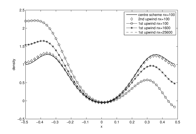
Figure 2: Density calculated by using the three schemes.

The numerical solution of the 2nd order upwind scheme with $N_{x}=100$ is consistent with that of the 1st order upwind scheme with $N_{x}=25600$, and the result of the central scheme is more symmetric. The difference between two second-order method is reflected from Figure 2, where the density obtained by using the second-order upwind finite-difference method with $N_{x}=100$ is almost coincident with that obtained by using the first-order upwind finite-difference method with $N_{x}=25600$ while the density obtained by using the central scheme is more symmetric.

Figure 2 gives us an intuitive understanding of the symmetry of the solution. Next, we will define a symmetry error to compare the three schemes. Define the symmetry error to be

$$e_{\rm sym}=\int\,\mathrm{d}v\int\,\mathrm{d}x|f(x,v)-f(-x,v)|.$$ (3.10)

Numerically, the symmetry error can be approximated by

$$\tilde{e}_{\rm sym}=\sum_{i}\sum_{j}|f_{i}(x_{j})-f_{i}(-x_{j})|\Delta x.$$ (3.11)

The numerical symmetry errors obtained by using different schemes are collected in Table 1. It can be seen that the numerical solution obtained by using the first order upwind scheme becomes more and more symmetric as refining the mesh, the symmetry error of the 2nd order upwind scheme with $N_{x}=100$ is about the same with the 1st order upwind scheme with $N_{x}=25600$, and the solution obtained by the central scheme is perfectly symmetric due to the symmetry of the scheme itself. These are consistent with the results in Figure 2.

$N_{x}$	100	400	1600	6400	25600
1st upwind	1.03	0.7666	0.4185	0.1502	0.0422
2nd upwind	0.0462	7.446e-4	1.151e-5
central	2.5966e-16

Table 1: Symmetry errors of the three schemes

4 Conclusion

For the problem whether the solution of the stationary Wigner equation with inflow boundary conditions will be symmetric if the potential is symmetric in [8], we give a rigorous proof based on [1] under mild assumption on the regularity of the potential. It is concluded that a certain kind of continuous Wigner equation with inflow boundary condition can be reduced to the discrete-velocity case, thus is well-posed. Furthermore, we numerically studied the example in [8] and pointed out that the numerical solution will converge to the exact solution with symmetry, even when the numerical scheme adopted is not symmetric if only accuracy is enough.

References

- [1] A. Arnold, H. Lange, and P.F. Zweifel. A discrete-velocity, stationary Wigner equation. J. Math. Phys., 41(11):7167–7180, 2000.
- [2] W. Cai. Computational methods for electromagnetic phenomena: electrostatics in solvation, scattering, and electron transport. Cambridge Univ. Press, Cambridge, U.K, 2013.
- [3] W.R. Frensley. Wigner function model of a resonant-tunneling semiconductor device. Phys. Rev. B, 36:1570–1580, 1987.
- [4] K.L. Jensen and F.A. Buot. Numerical aspects on the simulation of I‐V characteristics and switching times of resonant tunneling diodes. J. Appl. Phys., 67:2153–255, 1990.
- [5] Y. Katznelson. An Introduction to Harmonic Analysis. Dover, New York, 2nd edition, 1976.
- [6] P.A. Markowich, N.J. Mauser, and F. Poupaud. A Wigner‐function approach to (semi)classical limits: Electrons in a periodic potential. J. Math. Phys., 35:1066–1094, 1994.
- [7] A. Pazy. Semigroups of Linear Operators and Applications to Partial Differential Equations. Springer, New York, 2nd edition, 1992.
- [8] D. Taj, L. Genovese, and F. Rossi. Quantum-transport simulations with the wigner-function formalism: Failure of conventional boundary-condition schemes. Europhys. Lett., 74(6):1060–1066, 2006.
- [9] E. Wigner. On the quantum correction for thermodynamic equilibrium. Phys. Rev., 40(5):749–759, Jun 1932.