Number theoretic applications of a class of Cantor series fractal functions, I

Abstract.

Suppose that $(P,Q)\in\mathbb{N}_{2}^{\mathbb{N}}\times\mathbb{N}_{2}^{\mathbb{N}}$ and $x=E_{0}.E_{1}E_{2}\cdots$ is the $P$-Cantor series expansion of $x\in\mathbb{R}$. We define $\psi_{P,Q}(x):=\sum_{n=1}^{\infty}\frac{\min(E_{n},q_{n}-1)}{q_{1}\cdots q_{n}}$. The functions $\psi_{P,Q}$ are used to construct many pathological examples of normal numbers. These constructions are used to give the complete containment relation between the sets of $Q$-normal, $Q$-ratio normal, and $Q$-distribution normal numbers and their pairwise intersections for fully divergent $Q$ that are infinite in limit. We analyze the Hölder continuity of $\psi_{P,Q}$ restricted to some judiciously chosen fractals. This allows us to compute the Hausdorff dimension of some sets of numbers defined through restrictions on their Cantor series expansions. In particular, the main theorem of a paper by Y. Wang et al. [29] is improved.

Properties of the functions $\psi_{P,Q}$ are also analyzed. Multifractal analysis is given for a large class of these functions and continuity is fully characterized. We also study the behavior of $\psi_{P,Q}$ on both rational and irrational points, monotonicity, and bounded variation. For different classes of ergodic shift invariant Borel probability measures $\mu_{1}$ and $\mu_{2}$ on $\mathbb{N}_{2}^{\mathbb{N}}$, we study which of these properties $\psi_{P,Q}$ satisfies for $\mu_{1}\times\mu_{2}$-almost every $(P,Q)\in\mathbb{N}_{2}^{\mathbb{N}}\times\mathbb{N}_{2}^{\mathbb{N}}$. Related classes of random fractals are also studied.

1. Introduction

The study of normal numbers and other statistical properties of real numbers with respect to large classes of Cantor series expansions was first studied by P. Erdös and A. Rényi. This early work was done by P. Erdös and A. Rényi in [7] and [8] and by A. Rényi in [19], [20], and [21]. One of the main goals of this paper is to greatly expand upon their work and that of several other authors. Applications to normal numbers are discussed in Section 3.

The $Q$-Cantor series expansion, first studied by G. Cantor in [4], is a natural generalization of the $b$-ary expansion. Let $\mathbb{N}_{k}:=\mathbb{Z}\cap[k,\infty)$. If $Q\in\mathbb{N}_{2}^{\mathbb{N}}$, then we say that $Q$ is a basic sequence. Given a basic sequence $Q=(q_{n})_{n=1}^{\infty}$, the $Q$-Cantor series expansion of a real $x$ in $\mathbb{R}$ is the (unique) expansion of the form

(1.1) $$x=E_{0}+\sum_{n=1}^{\infty}\frac{E_{n}}{q_{1}q_{2}\ldots q_{n}}$$

where $E_{0}=\left\lfloor x\right\rfloor$ and $E_{n}$ is in $\{0,1,\ldots,q_{n}-1\}$ for $n\geq 1$ with $E_{n}\neq q_{n}-1$ infinitely often. We abbreviate (1.1) with the notation $x=E_{0}.E_{1}E_{2}E_{3}\ldots$ w.r.t. $Q$.

Clearly, the $b$-ary expansion is a special case of (1.1) where $q_{n}=b$ for all $n$. If one thinks of a $b$-ary expansion as representing an outcome of repeatedly rolling a fair $b$-sided die, then a $Q$-Cantor series expansion may be thought of as representing an outcome of rolling a fair $q_{1}$ sided die, followed by a fair $q_{2}$ sided die and so on.

Let $x=E_{0}.E_{1}E_{2}\cdots$ w.r.t. $P$. If there are no values $n$ such that $E_{n}=0$ or $E_{n}=p_{n}-1$, then we let $\rho_{P}(x):=0$. Otherwise, set $\rho_{P}(x):=\sup\{k\in\mathbb{N}:\exists n\in\mathbb{N}\hbox{ such that }E_{n+t}\in\{0,p_{n+t}-1\}\forall t\in[0,k-1]\}$. For $k\in\mathbb{N}\cup\{0,\infty\}$, put $\mathscr{W}_{P}^{(k)}:=\{x\in\mathbb{R}:\rho_{P}(x)\leq k\}$ and

$$\mathscr{Z}_{P,Q}^{(k)}:=\{x=0.E_{1}E_{2}\cdots\hbox{ w.r.t. }P:E_{n}<\min(p_{n},q_{n})\}\cap\mathscr{W}_{P}^{(k)}\cap\left(\psi_{P,Q}\right)^{-1}\left(\mathscr{W}_{Q}^{(k)}\right).$$

Definition 1.1.

Let $(P,Q)\in\mathbb{N}_{2}^{\mathbb{N}}\times\mathbb{N}_{2}^{\mathbb{N}}$ and suppose that $x=E_{0}.E_{1}E_{2}\cdots$ w.r.t. $P$. We define

$$\psi_{P,Q}(x):=\sum_{n=1}^{\infty}\frac{\min(E_{n},q_{n}-1)}{q_{1}\cdots q_{n}}\hbox{ and }\phi_{P,Q}^{(k)}:=\psi_{P,Q}\Big{|}_{\mathscr{Z}_{P,Q}^{(k)}}.$$

The study of the functions $\psi_{P,Q}$ and $\phi_{P,Q}^{(k)}$ and their applications to digital problems involving Cantor series expansions form the core of this paper. Let $Q\in\mathbb{N}_{2}^{\mathbb{N}}$ and let $\mathscr{N}(Q),\mathscr{RN}(Q)$, and $\mathscr{DN}(Q)$ be the sets of $Q$-normal numbers, $Q$-ratio normal numbers, and $Q$-distribution normal numbers, respectively. The original motivation for the author to study the functions $\psi_{P,Q}$ was to study the set $\mathscr{RN}(Q)\cap\mathscr{DN}(Q)\backslash\mathscr{N}(Q)$ and the sets constructed in the sequel to this paper by B. Li and the author [14]. One of the more surprising applications of the methods introduced in this paper is that for every $k\geq 2$, there exists a basic sequence $Q$ and a real number $x$ that is $Q$-normal of order $k$, but not $Q$ normal of any order $1,2,\cdots$, or $k-1$. Explicit examples of computable basic sequences $Q$ and computable real numbers $x$ with this property are given in [14].

The basic sequence $Q$ constructed in Section 3.2 is a computable sequence and the member of $\mathscr{RN}(Q)\cap\mathscr{DN}(Q)\backslash\mathscr{N}(Q)$ constructed in the same section is a computable real number. No deep knowledge of computability theory will be used and any time we make such a claim there will exist a simple algorithm to compute the number under consideration to any degree of precision. Section 3 is devoted to understanding the relationship between $\mathscr{N}(Q),\mathscr{RN}(Q)$, and $\mathscr{DN}(Q)$ and intersections thereof. We refer to the directed graph in Figure 1 for the complete containment relationships between these notions when $Q$ is infinite in limit and fully divergent. The vertices are labeled with all possible intersections of one, two, or three choices of the sets $\mathscr{N}(Q)$, $\mathscr{RN}(Q)$, and $\mathscr{DN}(Q)$. The set labeled on vertex $A$ is a subset of the set labeled on vertex $B$ if and only if there is a directed path from $A$ to $B$. For example, $\mathscr{N}(Q)\cap\mathscr{DN}(Q)\subseteq\mathscr{RN}(Q)$, so all numbers that are $Q$-normal and $Q$-distribution normal are also $Q$-ratio normal. A block is an ordered tuple of non-negative integers, a block of length $k$ is an ordered $k$-tuple of integers, and block of length $k$ in base $b$ is an ordered $k$-tuple of integers in $\{0,1,\ldots,b-1\}$.

The following is the main result of Section 3.

Theorem 1.2.

Figure 1 represents the complete containment relationship for basic sequences $Q$ that are infinite in limit and fully divergent.

Figure 1.

Suppose that $M=(m_{t})_{t}$ is an increasing sequence of positive integers. Let $N_{M,n}^{Q}(B,x)$ be the number of occurrences of the block $B$ at positions $m_{t}$ for $m_{t}\leq n$ in the $Q$-Cantor series expansion of $\{x\}$. For $m_{t}=t$ and $M=(m_{t})$, let $N_{n}^{Q}(B,x):=N_{M,n}^{Q}(B,x)$. We must also discuss the set of real numbers who have more than one expansion of the form (1.1) if we do not restrict $E_{n}<q_{n}-1$ infinitely often. These are precisely the points $x=E_{0}.E_{1}E_{2}\cdots E_{n}$ w.r.t. $Q$. We note that if $x$ is of this form, then

$$x=E_{0}+\sum_{j=1}^{n-1}\frac{E_{j}}{q_{1}\cdots q_{j}}+\frac{E_{n}-1}{q_{1}\cdots q_{n}}+\sum_{j=n+1}^{\infty}\frac{q_{j}-1}{q_{1}\cdots q_{j}}.$$

It should be noted that the distinction between these numbers will play a critical role in studying the properties of $\psi_{P,Q}$ as well as applications towards other problems. Thus, for a basic sequence $Q$, we let $\mathscr{U}_{Q}:=\{x=E_{0}.E_{1}E_{2}\cdots\hbox{ w.r.t. }Q:E_{n}\neq 0\hbox{ infinitely often}\}$ be the set of points with unique $Q$-Cantor series expansion and let $\mathscr{NU}_{Q}:=\mathbb{R}\backslash\mathscr{U}_{Q}$. The following theorem is not difficult to prove but will be of fundamental importance for the normal number constructions in this paper, the sequel to this paper with B. Li [14], and those in planned future projects.

Theorem 1.3.

Suppose that $M=(m_{t})$ is an increasing sequence of positive integers and $Q_{1}=(q_{1,n}),Q_{2}=(q_{2,n}),\cdots,Q_{j}=(q_{j,n})$ are basic sequences and infinite in limit. Set

$$\Psi_{j}(x)=\left(\psi_{Q_{j-1},Q_{j}}\circ\psi_{Q_{j-2},Q_{j-1}}\circ\cdots\circ\psi_{Q_{1},Q_{2}}\right)(x).$$

If $x=E_{0}.E_{1}E_{2}\cdots$ w.r.t $Q_{1}$ satisfies $E_{n}<\min_{2\leq r\leq j}(q_{r,n}-1)$ for infinitely many $n$, then $\Psi_{j}(x)\in\mathscr{U}_{Q_{j}}$ and for every block $B$

$$N_{M,n}^{Q_{j}}\left(B,\Psi_{j}(x)\right)=N_{M,n}^{Q_{1}}(B,x)+O(1).$$

The functions $\psi_{P,Q}$ and $\phi_{P,Q}^{(k)}$ are interesting in their own right. There is a vast literature studying functions with pathological properties. An early example due to Weierstrauss is of a class of continuous and nowhere differentiable functions. The study of other functions such as the Cantor function, Minwoski’s question mark function, and the Takagi function also provides motivation for Section 2. We give only a few references as relevant starting points: [1], [6], and [12]. We also mention that other fractal functions defined through Cantor series have been studied by H. Wang and Z. Xu in [27] and [28]. However, these functions are quite different from the $\psi_{P,Q}$ and $\phi_{P,Q}^{(k)}$ functions we study in this paper.

For a set $S\subseteq\mathbb{R}$, we will let $\lambda(S)$ denote the Lebesgue measure of $S$ and $\hbox{dim${}_{\hbox{H}}$}\left(S\right),\hbox{dim${}_{\hbox{P}}$}\left(S\right)$, and $\hbox{dim${}_{\hbox{B}}$}\left(S\right)$ will denote the Hausdorff, packing, and box dimensions of $S$, respectively. In Section 2, we will examine many properties of the functions $\psi_{P,Q}$ including, but not limited to, rationality, continuity, and bounded variation. We will also study the level sets of $\psi_{P,Q}$ and multifractal analysis of $\psi_{P,Q}$. For simplicity, we will only consider the level sets of $\psi_{P,Q}$ in $(0,1]$ as $\psi_{P,Q}$ is $1$-periodic and $\psi_{P,Q}(x)=0$ if and only if $x\in\mathbb{Z}$. For $w\in(0,1]$, put

$$\mathscr{L}_{P,Q}\left(w\right):=\{x\in(0,1):\psi_{P,Q}(x)=w\}.$$

For $\alpha\in[0,1]$, let

$$\mathscr{V}_{P,Q}\left(\alpha\right):=\{w\in\psi_{P,Q}((0,1)):\hbox{dim${}_{\hbox{H}}$}\left(\mathscr{L}_{P,Q}\left(w\right)\right)=\alpha\}$$

be a level set of the function $\hbox{dim${}_{\hbox{H}}$}\left(\mathscr{L}_{P,Q}\left(\cdot\right)\right)$. Let $\tau_{n}=n(n+1)/2$ be the $n$’th triangular number. An eventually non-decreasing sequence of real numbers $(s_{n})$ grows nicely if

$$\lim_{n\to\infty}\frac{\log s_{\tau_{n+2}}}{\log s_{\tau_{n}}}=1.$$

We will prove the following theorem.

Theorem 1.4.

For $(P,Q)\in\mathbb{N}_{2}^{\mathbb{N}}\times\mathbb{N}_{2}^{\mathbb{N}}$, let $r_{n}=p_{n}-q_{n}$. If $(p_{n}),(q_{n})$, and $(r_{n})$ grow nicely, $p_{n}>q_{n}$ for all natural numbers $n$, and

$$\lim_{n\to\infty}\frac{\log r_{n}}{\log p_{n}}=\gamma\in(0,1],$$

then for all $\alpha\in[0,1]$

$$\hbox{dim${}_{\hbox{H}}$}\left(\mathscr{V}_{P,Q}\left(\alpha\right)\right)\geq 1-\frac{\alpha}{\gamma}.$$

Thus, $\hbox{dim${}_{\hbox{H}}$}\left(\mathscr{V}_{P,Q}\left(\alpha\right)\right)>0$ if $0\leq\alpha<\gamma$.

While some properties such as continuity may easily be described for arbitrary choices of $P$ and $Q$, others will be too difficult to analyze for completely arbitrary choices. Thus, for certain classes of ergodic and shift-invariant Borel probability measures $\mu_{1},\mu_{2}$ on $\mathbb{N}_{2}^{\mathbb{N}}$ we will study these properties for $\mu_{1}\times\mu_{2}$-almost every $(P,Q)\in\mathbb{N}_{2}^{\mathbb{N}}\times\mathbb{N}_{2}^{\mathbb{N}}$. This will naturally give rise to many random fractals that we will consider. We also include graphs of $\psi_{P,Q}$ for many choices of $P$ and $Q$ in Figure 2.

The Hölder and Lipschitz continuity of $\phi_{P,Q}^{(k)}$ is explored in Section 2.6. This allows us to compute the Hausdorff dimension of some fractals defined through digital restrictions of Cantor series expansions in Section 4. Additionally, we will use the results of Section 2.6 to improve the main theorem in the paper [29] by Y. Wang et al and a result of the author in [15]. For the remainder of this paper, we will assume the convention that the empty sum is equal to $0$ and the empty product is equal to $1$.

2. The functions $\psi_{P,Q}$ and $\phi_{P,Q}^{(k)}$

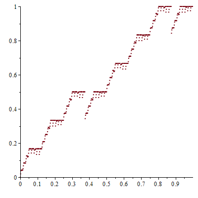
(a) $\begin{subarray}{c}p_{n}=2^{n}\\ q_{n}=n+1\end{subarray}$

(b) $\begin{subarray}{c}p_{n}=n+1\\ q_{n}=2^{n}\end{subarray}$

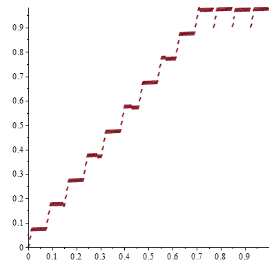
(c) $\begin{subarray}{c}P=(13,13,7,9,2,7,2,7,5,17,\cdots)\\ Q=(10,3,15,12,15,6,7,9,6,17,\cdots)\end{subarray}$

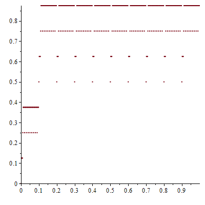
(d) $\begin{subarray}{c}p_{n}=10\\ q_{n}=2\end{subarray}$

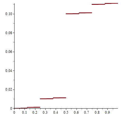
(e) $\begin{subarray}{c}p_{n}=2\\ q_{n}=10\end{subarray}$

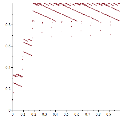
(f) $\begin{subarray}{c}P=(11,15,13,8,13,14,2,8,4,5,\cdots)\\ Q=(3,2,8,7,9,2,11,8,11,12,\cdots)\end{subarray}$

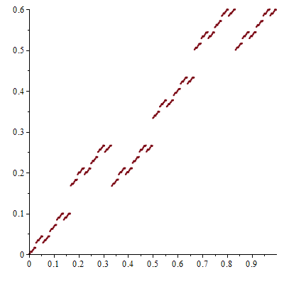
(g) $\begin{subarray}{c}P=(2,3,2,3,2,3,2,3,2,3,\cdots)\\ Q=(3,2,3,2,3,2,3,2,3,2,\cdots)\end{subarray}$

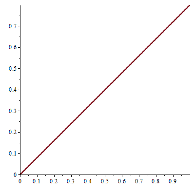
(h) $\begin{subarray}{c}P=(64,73,9,173,169,61,179,43,182,108,\cdots)\\ Q=(80,83,10,190,151,11,101,132,41,77,\cdots)\end{subarray}$

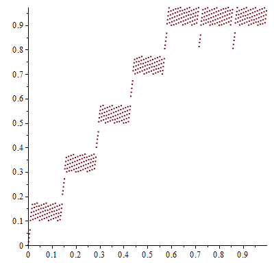
(i) $\begin{subarray}{c}P=(7,15,9,2,7,3,4,9,4,4,\cdots)\\ Q=(5,2,12,2,15,15,12,8,8,12,\cdots)\end{subarray}$

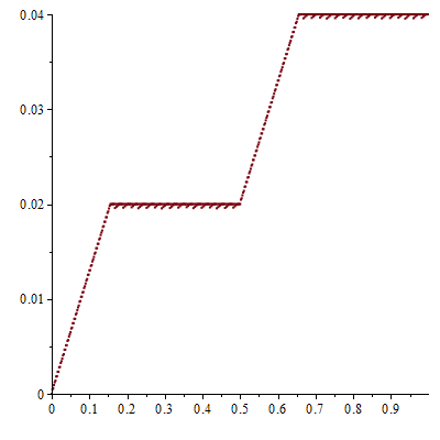
(j) $\begin{subarray}{c}P=(2,137,103,87,24,143,54,170,100,182)\\ Q=(50,43,33,48,50,15,92,164,23,33)\end{subarray}$

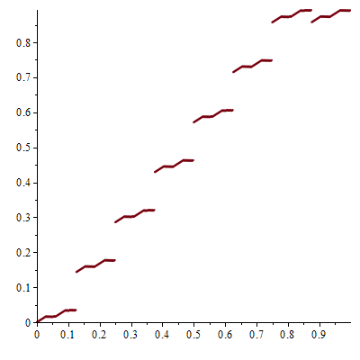
(k) $\begin{subarray}{c}P=(8,2,10,10,9,9,3,10,6,5,\cdots)\\ Q=(7,8,5,3,7,5,10,4,10,9,\cdots)\end{subarray}$

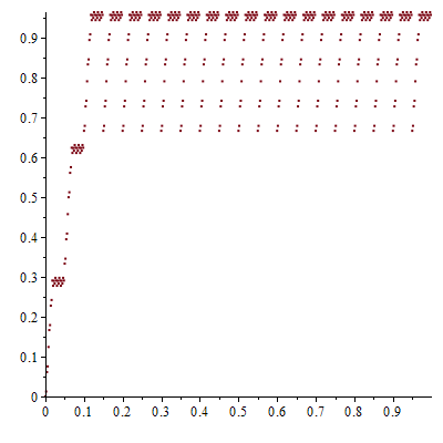
(l) $\begin{subarray}{c}P=(20,15,3,19,7,19,19,19,11,5,\cdots)\\ Q=(3,6,8,4,11,3,9,15,17,8,\cdots)\end{subarray}$

Figure 2. Graphs of $\psi_{P,Q}$ for different choices of $P$ and $Q$ plotted with $500$ pixels each. Most graphs without an explicit formula for $p_{n}$ and $q_{n}$ were generated randomly.

For $Q\in\mathbb{N}_{2}^{\mathbb{N}}$ and a sequence of natural numbers $(a_{j})$, define

$$\mathscr{R}_{(a_{j})}(Q):=\{x=0.E_{1}E_{2}\cdots\hbox{ w.r.t. }Q:E_{j}<a_{j}\}.$$

We note the following result due to H. Wegmann in [30]:

Theorem 2.1.

If $Q=(q_{n})\in\mathbb{N}_{2}^{\mathbb{N}}$ and $\lim_{n\to\infty}\frac{\log q_{n}}{\log q_{1}\cdots q_{n}}=0$, then

$$\hbox{dim${}_{\hbox{H}}$}\left(\mathscr{R}_{(a_{j})}(Q)\right)=\liminf_{n\to\infty}\frac{\log\prod_{j=1}^{n}\min(a_{j},q_{j})}{\log\prod_{j=1}^{n}q_{j}}.$$

The next theorem directly follows from Definition 1.1 and Theorem 2.1.

Theorem 2.2.

If $(P,Q)\in\mathbb{N}_{2}^{\mathbb{N}}\times\mathbb{N}_{2}^{\mathbb{N}}$, then

$$\psi_{P,Q}(\mathbb{R})=\mathscr{R}_{(\min(p_{j},q_{j}))}(Q)\subseteq\left[0,\sum_{n=1}^{\infty}\frac{\min(p_{n}-1,q_{n}-1)}{q_{1}\cdots q_{n}}\right]\hbox{ and }\lambda\left(\psi_{P,Q}(\mathbb{R})\right)=\prod_{j=1}^{\infty}\frac{\min(p_{j},q_{j})}{q_{j}}.$$

Moreover, if $\lim_{n\to\infty}\frac{\log q_{n}}{\log q_{1}\cdots q_{n}}=0$, then

$$\hbox{dim${}_{\hbox{H}}$}\left(\psi_{P,Q}(\mathbb{R})\right)=\liminf_{n\to\infty}\frac{\log\prod_{j=1}^{n}\min(p_{j},q_{j})}{\log\prod_{j=1}^{n}q_{j}}.$$

Thus, the range of $\psi_{P,Q}$ can be anywhere from the interval $[0,1]$ to a Cantor set. Given $Q\in\mathbb{N}_{2}^{\mathbb{N}}$, let $\mathscr{I}=(I_{n})$, where $I_{n}\subseteq\{0,1,\cdots,q_{n}-1\}$. For the rest of this paper, define $\mathscr{R}_{\mathscr{I}}(Q)$ by

$$\mathscr{R}_{\mathscr{I}}(Q):=\left\{x=\sum_{n=1}^{\infty}\frac{E_{n}}{q_{1}q_{2}\ldots q_{n}}:E_{j}\in I_{j}\right\}.$$

The proof of Theorem 2.1 presented in [30] can trivially be modified to arrive at the following generalization of Theorem 2.1 that will frequently be used in this paper.

Theorem 2.3.

Suppose that $Q=(q_{n})\in\mathbb{N}_{2}^{\mathbb{N}},\lim_{n\to\infty}\frac{\log q_{n}}{\log q_{1}\cdots q_{n}}=0,I_{j}\subseteq\{0,1,\cdots,q_{j}-1\}$, and $\mathscr{I}=(I_{n})$. Then

$$\hbox{dim${}_{\hbox{H}}$}\left(\mathscr{R}_{\mathscr{I}}(Q)\right)=\liminf_{n\to\infty}\frac{\log\prod_{j=1}^{n}|I_{j}|}{\log\prod_{j=1}^{n}q_{j}}.$$

It should be noted that the sets $\mathscr{R}_{\mathscr{I}}(Q)$ are homogenous Moran sets. Using corollary 3.1 from Feng et al. [9], we have the following result connecting the Hausdorff, packing, and box dimensions of $\mathscr{R}_{\mathscr{I}}(Q)$.

Lemma 2.4.

If

(2.1) $$\liminf_{n\to\infty}\frac{\log\prod_{j=1}^{n}|I_{j}|}{\log\prod_{j=1}^{n+1}|q_{j}|-\log|I_{n+1}|}=\limsup_{n\to\infty}\frac{\log\prod_{j=1}^{n+1}|I_{j}|}{\log\prod_{j=1}^{n}|q_{j}|+\log|I_{n+1}|},$$

then $\hbox{dim${}_{\hbox{H}}$}\left(\mathscr{R}_{\mathscr{I}}({Q})\right)=\hbox{dim${}_{\hbox{P}}$}\left(\mathscr{R}_{\mathscr{I}}({Q})\right)=\hbox{dim${}_{\hbox{B}}$}\left(\mathscr{R}_{\mathscr{I}}({Q})\right)$.

Lastly, we give a proof of Theorem 1.3.

Proof of Theorem 1.3.

Let $B=(b_{1},b_{2},\cdots,b_{k})$. We use induction on $j$. The base case $j=1$ is trivial. Suppose now that $j\geq 2$ and $N_{M,n}^{Q_{j-1}}\left(B,\Psi_{j-1}(x)\right)=N_{M,n}^{Q_{1}}(B,x)+O(1).$ Put $b=\max(b_{1},b_{2},\cdots,b_{k})$ and let $\Psi_{j-1}(x)=F_{0}.F_{1}F_{2}\cdots$ w.r.t. $Q_{j-1}$ and $\Psi_{j}(x)=G_{0}.G_{1}G_{2}\cdots$ w.r.t. $Q_{j}$. Since $\min(E_{n},q_{2}-1,\cdots,q_{j-1}-1)\leq E_{n}<q_{n,j}-1$ for infinitely many $n$, we know that $\Psi_{j}(x)\in\mathscr{U}_{Q_{j}}$. Let $t$ be large enough that $b<\min_{1\leq r\leq j}(q_{j,n}-1)$ for every $n\geq t$. Since $\Psi_{j}(x)\in\mathscr{U}_{Q_{j}}$, we know for $n\geq t$ that $G_{n}\in\{0,1,\cdots,b\}$ if and only if $F_{n}\in\{0,1,\cdots,b\}$. Thus,

$$N_{M,n}^{Q_{j-1}}\left(B,\Psi_{j-1}(x)\right)-N_{M,t}^{Q_{j-1}}\left(B,\Psi_{j-1}(x)\right)\leq N_{M,n}^{Q_{j}}\left(B,\Psi_{j}(x)\right)$$

$$\leq \left(N_{M,n}^{Q_{j-1}}\left(B,\Psi_{j-1}(x)\right)-N_{M,t}^{Q_{j-1}}\left(B,\Psi_{j-1}(x)\right)\right)+t,$$

so $N_{M,n}^{Q_{j}}\left(B,\Psi_{j}(x)\right)=N_{M,n}^{Q_{1}}(B,x)+O(1)$ and Theorem 1.3 is proven. ∎

2.1. Level Sets and Multifractal Analysis of $\psi_{P,Q}$

We wish to examine the range of $\psi_{P,Q}$ beyond what was discussed in Theorem 2.2. Our main tool will be Theorem 2.3. For this subsection, we will assume that $\lim_{n\to\infty}\frac{p_{n}}{p_{1}\cdots p_{n}}=0$ so that we may use Theorem 2.3. We will see in Section 2.5 that the level sets $\mathscr{L}_{P,Q}\left(w\right)$ are always empty, a single point, or a totally disconnected set.

The next theorem follows directly from the definition of the Cantor series expansions and $\psi_{P,Q}$ and gives a complete characterization of the level sets of $\psi_{P,Q}$. None of the following statements are difficult to prove so we omit their proofs.

Theorem 2.5.

Suppose that $w\in(0,1]$ and $x\in\mathscr{L}_{P,Q}\left(w\right)$. We write $w=E_{0}.E_{1}E_{2}\cdots$ w.r.t. $Q$ and $x=0.F_{1}F_{2}\cdots\hbox{ w.r.t. }P$.

1. If $E_{n}\in[0,q_{n}-2]$ and there exists $m>n$ such that $E_{m}\neq 0$, then $F_{n}=E_{n}$.

2. If $E_{n}=q_{n}-1$ and there exists $m>n$ such that $E_{m}\neq 0$, then $F_{n}\in[q_{n}-1,p_{n}-1]$.

3. If $w\in\mathscr{NU}_{Q}\cap(0,1)$ and $n=\sup\{t\in\mathbb{N}:E_{t}>0\}$, then $\mathscr{L}_{P,Q}\left(w\right)=A\cup B$, where

   $$A=\{\zeta=0.G_{1}\cdots G_{n}\hbox{ w.r.t }P:\psi_{P,Q}(\zeta)=w\}\hbox{ and}$$

   $$B=\Bigg{\{}0.G_{1}\cdots G_{n-1}(E_{n}-1)G_{n+1}\cdots\hbox{ w.r.t }P:\ G_{m}\in[q_{m}-1,p_{m}-1]\forall m>n$$

   $$\hbox{ and }\psi_{P,Q}\left(\sum_{j=1}^{n-1}\frac{G_{j}}{p_{1}\cdots p_{j}}\right)=\sum_{j=1}^{n-1}\frac{E_{j}}{q_{1}\cdots q_{j}}\Bigg{\}}.$$

   Clearly, the set $A$ is at most finite although the set $B$ may be quite large. Also

   $$\mathscr{L}_{P,Q}\left(1\right)=\left\{0.G_{1}G_{2}\cdots\hbox{ w.r.t. }P:G_{m}\in[q_{m}-1,p_{m}-1]\forall m\in\mathbb{N}\right\}.$$

4. If $w\in\mathscr{U}_{Q}$, then $\mathscr{L}_{P,Q}\left(w\right)=\emptyset$ if and only if there exists a natural number $n$ such that $E_{n}\geq p_{n}$.

5. If there exists $n$ with $p_{n}<q_{n}$, then $\mathscr{L}_{P,Q}\left(w\right)=~{}\emptyset$ for all $w>\sum_{n=1}^{\infty}\frac{\min(p_{n}-1,q_{n}-1)}{q_{1}\cdots q_{n}}$.

6. If $p_{n}>q_{n}$ for at most finitely many $n$, then $\mathscr{L}_{P,Q}(w)$ is finite for all $w\in\psi_{P,Q}((0,1))$.

7. If $p_{n}\leq q_{n}$ for all $n$, then $\psi_{P,Q}$ is injective and increasing.

For $w=0.E_{1}E_{2}\cdots$ w.r.t. $Q$, set

$$\omega_{n}(w)=\left\{\begin{array}[]{ll}1&\textrm{if $E_{n}\in[0,q_{n}-2]$}\\ p_{n}-q_{n}+1&\textrm{if $E_{n}=q_{n}-1$}\\ 0&\textrm{if $E_{n}\geq p_{n}$}\\ \end{array}\right..$$

Theorem 2.6.

Let $w=0.E_{1}E_{2}\cdots$ w.r.t. $Q$. If $w\in\mathscr{U}_{Q}$, then

(2.2) $$\lambda\left(\mathscr{L}_{P,Q}\left(w\right)\right)=\prod_{j=1}^{\infty}\frac{\omega_{j}(w)}{p_{j}}\hbox{ and }\hbox{dim${}_{\hbox{H}}$}\left(\mathscr{L}_{P,Q}\left(w\right)\right)=\liminf_{n\to\infty}\frac{\log\prod_{j=1}^{n}\omega_{j}(w)}{\log\prod_{j=1}^{n}p_{j}}.$$

If $w\in\mathscr{NU}_{Q}$, $M=\inf\{t\in\mathbb{N}:E_{t}>0\}$, and $p_{n}\geq q_{n}$ for all $n>M$, then

$$\lambda\left(\mathscr{L}_{P,Q}\left(w\right)\right) =\left(\prod_{j=1}^{M-1}\frac{\omega_{j}(w)}{p_{j}}\right)\cdot\frac{1}{p_{M}}\cdot\left(\prod_{j=M+1}^{\infty}\frac{p_{j}-q_{j}+1}{p_{j}}\right)\hbox{ and }$$

$$\hbox{dim${}_{\hbox{H}}$}\left(\mathscr{L}_{P,Q}\left(w\right)\right) =\liminf_{n\to\infty}\frac{\log\prod_{j=M+1}^{n}\omega_{j}(w)}{\log\prod_{j=M+1}^{n}p_{j}}.$$

If $\mathscr{L}_{P,Q}\left(w\right)\neq\emptyset$ and (2.1) holds with

$$I_{n}=I_{n}(w)=\left\{\begin{array}[]{ll}\{E_{n}\}&\textrm{if $E_{n}\in[0,q_{n}-2]$}\\ \left[q_{n}-1,p_{n}-1\right]&\textrm{if $E_{n}=q_{n}-1$}\end{array}\right.,$$

then $\hbox{dim${}_{\hbox{H}}$}\left(\mathscr{L}_{P,Q}\left(w\right)\right)=\hbox{dim${}_{\hbox{P}}$}\left(\mathscr{L}_{P,Q}\left(w\right)\right)=\hbox{dim${}_{\hbox{B}}$}\left(\mathscr{L}_{P,Q}\left(w\right)\right)$.

Proof.

This follows from Theorem 2.3 and our characterization of the level sets of $\psi_{P,Q}$ in Theorem 2.5. The last part follows from Lemma 2.4. ∎

We will need the following basic lemmas to help prove Theorem 1.4.

Lemma 2.7.

Let $L$ be a real number and $(a_{n})_{n=1}^{\infty}$ and $(b_{n})_{n=1}^{\infty}$ be two sequences of positive real numbers such that

$$\sum_{n=1}^{\infty}b_{n}=\infty\hbox{ and }\lim_{n\to\infty}\frac{a_{n}}{b_{n}}=L.$$

Then

$$\lim_{n\to\infty}\frac{a_{1}+a_{2}+\ldots+a_{n}}{b_{1}+b_{2}+\ldots+b_{n}}=L.$$

Lemma 2.8.

Let $L$ be a real number and $(a_{n})_{n=1}^{\infty}$ and $(b_{n})_{n=1}^{\infty}$ be two sequences of positive integers. Let $(c_{t})_{t=1}^{\infty}$ be an increasing sequence of positive integers. Set $A_{t}=\sum_{n=c_{t}}^{c_{t+1}-1}a_{n}$ and $B_{t}=\sum_{n=c_{t}}^{c_{t+1}-1}b_{n}$. If $\lim_{t\to\infty}\frac{A_{1}+A_{2}+\cdots+A_{t}}{B_{1}+B_{2}+\cdots+B_{t}}=L,\ \sum_{t=1}^{\infty}A_{t}=\sum_{t=1}^{\infty}B_{t}=\infty,$ and $\lim_{t\to\infty}\frac{A_{t+1}}{A_{1}+A_{2}+\cdots+A_{t}}=\lim_{t\to\infty}\frac{B_{t+1}}{B_{1}+B_{2}+\cdots+B_{t}}=0$, then

$$\lim_{n\to\infty}\frac{a_{1}+a_{2}+\ldots+a_{n}}{b_{1}+b_{2}+\ldots+b_{n}}=L.$$

We also need

Lemma 2.9.

If $(s_{n})$ grows nicely, then $\lim_{n\to\infty}\frac{\log s_{n}}{\log s_{1}s_{2}\cdots s_{n}}=0$.

Proof.

Let $m\in\mathbb{N}$. For $t>m$ and $n\in[\tau_{t+1},\tau_{t+2})$

$$\frac{\log s_{n}}{\log s_{1}s_{2}\cdots s_{n}}\leq\frac{\log s_{\tau_{t+2}}}{\log\prod_{j=\tau_{t}}^{\tau_{t}+m}s_{j}}.$$

Since $(s_{n})$ is monotone

$$\lim_{n\to\infty}\frac{\log s_{n}}{\log s_{1}s_{2}\cdots s_{n}}\leq\lim_{t\to\infty}\frac{\log s_{\tau_{t+2}}}{\sum_{j=\tau_{t}}^{\tau_{t}+m}\log s_{j}}=\frac{1}{m}$$

and $\lim_{n\to\infty}\frac{\log s_{n}}{\log s_{1}s_{2}\cdots s_{n}}=0$. ∎

Proof of Theorem 1.4.

Let $\alpha<\gamma$ and $N$ be the smallest integer such that $p_{n}>q_{n}$, $q_{n}>2$, and $(p_{n}),(q_{n})$, and $(r_{n})$ are non-decreasing for all $n>N$. We will describe a set $S\subseteq(0,1]$ where $\hbox{dim${}_{\hbox{H}}$}\left(\mathscr{L}_{P,Q}\left(w\right)\right)=\alpha$ for all $w\in S$ and $\hbox{dim${}_{\hbox{H}}$}\left(S\right)=1-\frac{\alpha}{\gamma}$. Let

$$c_{t}=\sum_{j=1}^{t}\left\lceil\left(1-\frac{\alpha}{\gamma}\right)j\right\rceil+\left\lceil\frac{\alpha}{\gamma}j\right\rceil.$$

Set $M=\min\{t:c_{t}>N\}$,

$$I_{n}=\left\{\begin{array}[]{ll}\{0,1,\cdots,q_{n}-2\}&\textrm{if $n\in\left[c_{t},c_{t}+\left\lceil\left(1-\frac{\alpha}{\gamma}\right)t\right\rceil-1\right]$}\\ &\\ \{q_{n}-1\}&\textrm{if $n\in\left[c_{t}+\left\lceil\left(1-\frac{\alpha}{\gamma}\right)t\right\rceil,c_{t+1}-1\right]$}\\ \end{array}\right.,$$

$\mathscr{I}=(I_{n})$, and $S=\mathscr{R}_{\mathscr{I}}(Q)$. Let $w\in S$ and put

$$A_{t} =\left\lceil\frac{\alpha}{\gamma}t\right\rceil\log(r_{c_{t}}), A_{t}^{\prime}=\sum_{n=c_{t}}^{c_{t+1}-1}\log\omega_{n}(w)$$

$$B_{t} =\left(\left\lceil\left(1-\frac{\alpha}{\gamma}\right)t\right\rceil+\left\lceil\frac{\alpha}{\gamma}t\right\rceil\right)\log(p_{c_{t}}), B_{t}^{\prime}=\sum_{n=c_{t}}^{c_{t+1}-1}\log p_{n}.$$

Thus, $\lim_{t\to\infty}\frac{A^{\prime}_{t}}{A_{t}}=\lim_{n\to\infty}\frac{B^{\prime}_{t}}{B_{t}}=1$ since $(r_{n})$ and $(p_{n})$ are nice sequences. Since $(r_{n})$ is eventually monotone and $r_{n}\to\infty$

$$\lim_{t\to\infty}\frac{A_{t+1}}{A_{M}+\cdots+A_{t}}=\lim_{t\to\infty}\frac{\left\lceil\frac{\alpha}{\gamma}(t+1)\right\rceil\log r_{c_{t+1}}}{\sum_{j=M}^{t}\ {\left\lceil\frac{\alpha}{\gamma}j\right\rceil\log r_{c_{j}}}}\leq\lim_{t\to\infty}\frac{\left\lceil\frac{\alpha}{\gamma}(t+1)\right\rceil\log r_{c_{t+1}}}{\sum_{j=M}^{t}\ {\left\lceil\frac{\alpha}{\gamma}j\right\rceil\log r_{c_{t}}}}$$

$$=\lim_{t\to\infty}\frac{\left\lceil\frac{\alpha}{\gamma}(t+1)\right\rceil}{\sum_{j=M}^{t}\left\lceil\frac{\alpha}{\gamma}j\right\rceil}=\lim_{t\to\infty}\frac{t+1}{t(t+1)/2+O(t)}=0.$$

Similarly, it can be shown that $\lim_{t\to\infty}\frac{B_{t+1}}{B_{M}+\cdots+B_{t}}=0$, so by Lemma 2.7 and Lemma 2.8

(2.3) $$\lim_{n\to\infty}\frac{\sum_{j=c_{M}}^{n}\log\omega_{j}(w)}{\sum_{j=c_{M}}^{n}\log p_{j}}=\lim_{t\to\infty}\frac{A_{t}}{B_{t}}=\lim_{t\to\infty}\left(\frac{\left\lceil\frac{\alpha}{\gamma}t\right\rceil}{\left\lceil\left(1-\frac{\alpha}{\gamma}\right)t\right\rceil+\left\lceil\frac{\alpha}{\gamma}t\right\rceil}\cdot\frac{\log r_{c_{t}}}{\log p_{c_{t}}}\right)=\frac{\alpha}{\gamma}\cdot\gamma=\alpha.$$

By construction, $w\in\mathscr{U}_{Q}$. Thus, by (2.2), (2.3), and Lemma 2.9

$$\hbox{dim${}_{\hbox{H}}$}\left(\mathscr{L}_{P,Q}\left(w\right)\right)=\liminf_{n\to\infty}\frac{\log\prod_{j=c_{M}}^{n}\omega_{j}(w)}{\log\prod_{j=c_{M}}^{n}p_{j}}=\alpha.$$

Let

$$\upsilon_{n}=|I_{n}|=\left\{\begin{array}[]{ll}q_{n}-1&\textrm{if $n\in\left[c_{t},c_{t}+\left\lceil\left(1-\frac{\alpha}{\gamma}\right)t\right\rceil-1\right]$}\\ &\\ 1&\textrm{if $n\in\left[c_{t}+\left\lceil\left(1-\frac{\alpha}{\gamma}\right)t\right\rceil,c_{t+1}-1\right]$}\\ \end{array}\right..$$

Then, by Theorem 2.3 and Lemma 2.9

$$\hbox{dim${}_{\hbox{H}}$}\left(S\right)=\liminf_{n\to\infty}\frac{\log\prod_{j=c_{M}}^{n}\upsilon_{j}(w)}{\log\prod_{j=c_{M}}^{n}q_{j}}$$

A similar argument using Lemma 2.7 and Lemma 2.8 shows that $\hbox{dim${}_{\hbox{H}}$}\left(S\right)=1-\frac{\alpha}{\gamma}$. Thus, since $S\subseteq\mathscr{V}_{P,Q}\left(\alpha\right)$, we know that $\hbox{dim${}_{\hbox{H}}$}\left(\mathscr{V}_{P,Q}\left(\alpha\right)\right)\geq 1-\frac{\alpha}{\gamma}$ and $\hbox{dim${}_{\hbox{H}}$}\left(\mathscr{V}_{P,Q}\left(\alpha\right)\right)>0$ if $\alpha<\gamma$. ∎

Theorem 2.10.

Suppose that $p_{n}\geq q_{n}$ for all $n$ and $\sum\frac{q_{n}}{p_{n}}<\infty$. Then $\lambda\left(\mathscr{L}_{P,Q}\left(w\right)\right)>0$ if and only if $w\in\mathscr{NU}_{Q}\cap\psi_{P,Q}((0,1))$. Furthermore,

$$\sum_{w\in\psi_{P,Q}((0,1))}\lambda\left(\mathscr{L}_{P,Q}\left(w\right)\right)=\sum_{w\in\mathscr{NU}_{Q}\cap\psi_{P,Q}((0,1))}\lambda\left(\mathscr{L}_{P,Q}\left(w\right)\right)=\sum_{k=1}^{\infty}\frac{q_{k}-1}{p_{k}}\cdot\prod_{j=k+1}^{\infty}\left(1-\frac{q_{j}-1}{p_{j}}\right).$$

Proof.

We first note that $\sum\frac{q_{n}}{p_{n}}$ converges if and only if $\sum\frac{q_{n}-1}{p_{n}}$ converges. An argument that shows this is given in the proof of Theorem 2.18. Let $M=\inf\{t\in\mathbb{N}:E_{t}>0\}$. Then by (2.2) for $w=0.E_{1}E_{2}\cdots E_{M}$ w.r.t.

$$\lambda\left(\mathscr{L}_{P,Q}\left(w\right)\right)=\left(\prod_{j=1}^{M-1}\frac{\omega_{j}(w)}{p_{j}}\right)\cdot\frac{1}{p_{M}}\cdot\left(\prod_{j=M+1}^{\infty}\frac{p_{j}-q_{j}+1}{p_{j}}\right).$$

Since $\sum\frac{q_{n}-1}{p_{n}}$ converges,

$$\prod_{j=M+1}^{\infty}\frac{p_{j}-q_{j}+1}{p_{j}}=\prod_{j=M+1}^{\infty}\left(1-\frac{q_{j}-1}{p_{j}}\right)>0,$$

so $\lambda\left(\mathscr{L}_{P,Q}\left(w\right)\right)>0$. If $w\in\mathscr{U}_{Q}$, then

$$\lambda\left(\mathscr{L}_{P,Q}\left(w\right)\right)\leq\prod_{\begin{subarray}{c}1\leq j<\infty\\ E_{j}\neq q_{j}-1\end{subarray}}\frac{1}{p_{j}}=0,$$

by (2.2), so $\lambda\left(\mathscr{L}_{P,Q}\left(w\right)\right)=0$.

We will now evaluate $\sum_{w\in\mathscr{NU}_{Q}\cap\psi_{P,Q}((0,1))}\lambda\left(\mathscr{L}_{P,Q}\left(w\right)\right)$. Let

$$\xi_{n}(m)=\left\{\begin{array}[]{ll}1&\textrm{if $m\in[0,q_{n}-2]$}\\ p_{n}-q_{n}+1&\textrm{if $m=q_{n}-1$}\\ 0&\textrm{if $m\geq p_{n}$}\\ \end{array}\right.$$

and put $\Upsilon_{k}=\prod_{j=k+1}^{\infty}\frac{p_{j}-q_{j}+1}{p_{j}}=\prod_{j=k+1}^{\infty}\left(1-\frac{q_{j}-1}{p_{j}}\right)>0$. Then by (2.2)

$$\sum_{w\in\mathscr{NU}_{Q}\cap\psi_{P,Q}((0,1))}\lambda\left(\mathscr{L}_{P,Q}\left(w\right)\right)=\sum_{k=1}^{\infty}\sum_{\begin{subarray}{c}0\leq E_{1}\leq q_{1}-1\\ \cdots\\ 0\leq E_{k-1}\leq q_{k-1}-1\\ 1\leq E_{k}\leq q_{k}-1\end{subarray}}\lambda\left(\mathscr{L}_{P,Q}\left(\sum_{n=1}^{k}\frac{E_{n}}{q_{1}\cdots q_{n}}\right)\right)$$

$$= \sum_{k=1}^{\infty}\sum_{\begin{subarray}{c}0\leq E_{1}\leq q_{1}-1\\ \cdots\\ 0\leq E_{k-1}\leq q_{k-1}-1\\ 1\leq E_{k}\leq q_{k}-1\end{subarray}}\left(\prod_{j=1}^{k-1}\frac{\xi_{j}(E_{j})}{p_{j}}\right)\cdot\frac{1}{p_{k}}\cdot\left(\prod_{j=k+1}^{\infty}\frac{p_{j}-q_{j}+1}{p_{j}}\right)=\sum_{k=1}^{\infty}\left(\prod_{j=1}^{k-1}\sum_{E_{j}=0}^{q_{j}-1}\frac{\xi_{j}(E_{j})}{p_{j}}\right)\cdot\left(\sum_{E_{k}=1}^{q_{k}-1}\frac{1}{p_{k}}\cdot\Upsilon_{k}\right)$$

$$= \sum_{k=1}^{\infty}\left(\prod_{j=1}^{k-1}\frac{p_{j}}{p_{j}}\right)\cdot\frac{q_{k}-1}{p_{k}}\cdot\Upsilon_{k}=\sum_{k=1}^{\infty}\frac{q_{k}-1}{p_{k}}\cdot\prod_{j=k+1}^{\infty}\left(1-\frac{q_{j}-1}{p_{j}}\right).$$

∎

2.2. Measures on $\mathbb{N}_{2}^{\mathbb{N}}\times\mathbb{N}_{2}^{\mathbb{N}}$

Let $\tau:\mathbb{N}_{2}^{\mathbb{N}}\to\mathbb{N}_{2}^{\mathbb{N}}$ be the left shift on $\mathbb{N}_{2}^{\mathbb{N}}$ and let $\mathscr{M}^{e}\left(\mathbb{N}_{2}^{\mathbb{N}}\right)$ (resp. $\mathscr{M}^{w}\left(\mathbb{N}_{2}^{\mathbb{N}}\right)$) be the collection of all ergodic (resp. weakly mixing) $\tau$-invariant Borel probability measures on $\mathbb{N}_{2}^{\mathbb{N}}$. For $s,t\in\mathbb{N}$, set $\sigma_{s,t}=\tau^{s}\times\tau^{t}$ and $\sigma=\sigma_{1,1}$. If $\omega=((p_{1},p_{2},\cdots),(q_{1},q_{2},\cdots))\in\mathbb{N}_{2}^{\mathbb{N}}\times\mathbb{N}_{2}^{\mathbb{N}}$, then we write $\pi_{1}\left(\omega\right)=p_{1}$ and $\pi_{2}\left(\omega\right)=q_{1}$. Similarly, if $\omega=(p_{1},p_{2},\cdots)\in\mathbb{N}_{2}^{\mathbb{N}}$, then we let $\pi(\omega)=p_{1}$.

For $S\subseteq\mathbb{N}$, we say that $\nu\in\mathscr{M}^{w}\left(\mathbb{N}_{2}^{\mathbb{N}}\right)$ is positive on $S$ if $\nu\left(\left\{\omega\in\mathbb{N}_{2}^{\mathbb{N}}:\pi(\omega)\in S\right\}\right)>0$. $\nu$ is eventually positive if there exists $M$ such that $\nu$ is positive on $\{n\}$ for all $n\geq M$. If $\tau$ is weakly mixing, then $\sigma_{s,t}$ is ergodic and weakly mixing.

Lemma 2.11.

Suppose that $\mu_{1},\mu_{2}\in\mathscr{M}^{w}\left(\mathbb{N}_{2}^{\mathbb{N}}\right)$, $\mu=\mu_{1}\times\mu_{2}$, and

$$\max\left(\int\log\pi_{1}\left(\omega\right)\ d\mu(\omega),\int\log\pi_{2}\left(\omega\right)\ d\mu(\omega)\right)<\infty.$$

If $\int\log\pi_{1}\left(\omega\right)\ d\mu(\omega)>\alpha\cdot\int\log\pi_{2}\left(\omega\right)\ d\mu(\omega)$ for $\alpha>1$, then for all integers $k\geq 0$ and $\mu$-almost every $(P,Q)\in\mathbb{N}_{2}^{\mathbb{N}}\times\mathbb{N}_{2}^{\mathbb{N}}$

$$\lim_{n\to\infty}\frac{p_{1}\cdots p_{n}}{q_{1}\cdots q_{n\left\lfloor\alpha\right\rfloor+k}}=\infty.$$

If $\int\log\pi_{2}\left(\omega\right)\ d\mu(\omega)>\alpha\cdot\int\log\pi_{1}\left(\omega\right)\ d\mu(\omega)$ for $\alpha>1$, then for all integers $k\geq 0$ and $\mu$-almost every $(P,Q)\in\mathbb{N}_{2}^{\mathbb{N}}\times\mathbb{N}_{2}^{\mathbb{N}}$

$$\lim_{n\to\infty}\frac{p_{1}\cdots p_{n\left\lfloor\alpha\right\rfloor+k}}{q_{1}\cdots q_{n}}=0.$$

Proof.

For integers $s,t\geq 1$, set

$$f_{s,t,u,v}(\omega)=\sum_{j=0}^{t-1}\log\pi_{2}\left(\sigma^{j+v}(\omega)\right)-\sum_{j=0}^{s-1}\log\pi_{1}\left(\sigma^{j+u}(\omega)\right).$$

Let $t=\left\lfloor\alpha\right\rfloor$ and note that

$$\log\frac{q_{1}\cdots q_{nt+k}}{p_{1}\cdots p_{n}}=\log q_{1}\cdots q_{k}+\sum_{j=1}^{n}\log\left(\frac{\prod_{m=1}^{t}q_{(j-1)t+k+m}}{p_{j}}\right).$$

But $\sigma_{1,t}$ is ergodic, so for $\mu$-almost every $\omega\in\mathbb{N}_{2}^{\mathbb{N}}\times\mathbb{N}_{2}^{\mathbb{N}}$

$$\lim_{n\to\infty}\frac{1}{n}\log\frac{\pi_{2}\left(\omega\right)\cdots\pi_{2}\left(\sigma^{nt+k-1}(\omega)\right)}{\pi_{1}\left(\omega\right)\cdots\pi_{1}\left(\sigma^{n-1}{\omega}\right)}=\lim_{n\to\infty}\left(\frac{1}{n}\cdot\pi_{2}\left(\omega\right)\cdots\pi_{2}\left(\sigma^{k-1}(\omega)\right)+\frac{1}{n}\sum_{i=0}^{n-1}f_{1,t,0,k}\circ\sigma_{1,t}^{i}(\omega)\right)$$

$$= 0+\int f_{1,t,0,k}(\omega)\ d\mu(\omega)=\int\left(\sum_{j=0}^{t-1}\log\pi_{2}\left(\sigma^{j+k}(\omega)\right)-\log\pi_{1}\left(\omega\right)\right)\ d\mu(\omega)$$

$$= \left(\sum_{j=0}^{t-1}\int\log\pi_{2}\left(\sigma^{j+k}(\omega)\right)d\mu(\omega)\right)-\int\log\pi_{1}\left(\omega\right)\ d\mu(\omega)=\left(\sum_{j=0}^{t-1}\int\log\pi_{2}\left(\omega\right)d\mu(\omega)\right)-\int\log\pi_{1}\left(\omega\right)\ d\mu(\omega)$$

$$= t\int\log\pi_{2}\left(\omega\right)\ d\mu(\omega)-\int\log\pi_{1}\left(\omega\right)\ d\mu(\omega)<\alpha\int\log\pi_{2}\left(\omega\right)\ d\mu(\omega)-\int\log\pi_{1}\left(\omega\right)\ d\mu(\omega)<0.$$

Thus, for $\mu$-almost every $\omega\in\mathbb{N}_{2}^{\mathbb{N}}\times\mathbb{N}_{2}^{\mathbb{N}}$

$$\lim_{n\to\infty}\log\frac{\pi_{2}\left(\omega\right)\cdots\pi_{2}\left(\sigma^{nt+k-1}(\omega)\right)}{\pi_{1}\left(\omega\right)\cdots\pi_{1}\left(\sigma^{n-1}{\omega}\right)}=-\infty,$$

so

$$\lim_{n\to\infty}\frac{\pi_{2}\left(\omega\right)\cdots\pi_{2}\left(\sigma^{nt+k-1}(\omega)\right)}{\pi_{1}\left(\omega\right)\cdots\pi_{1}\left(\sigma^{n-1}({\omega})\right)}=0$$

and the first assertion follows. The second assertion is proven similarly. ∎

Lemma 2.12.

Suppose that $\max\left(\int\log\pi_{1}\left(\omega\right)\ d\mu(\omega),\int\log\pi_{2}\left(\omega\right)\ d\mu(\omega)\right)<\infty$ and $\alpha\in[0,1]$. If $\int\log\pi_{1}\left(\omega\right)\ d\mu(\omega)<\alpha\int\log\pi_{2}\left(\omega\right)\ d\mu(\omega)$, then

$$\lim_{n\to\infty}\frac{(p_{1}p_{2}\cdots p_{n})^{\alpha}}{q_{1}q_{2}\cdots q_{n}}\cdot\min(p_{n},q_{n})^{1-\alpha}=0$$

and

$$\lim_{n\to\infty}\frac{(p_{1}p_{2}\cdots p_{n+k})^{\alpha}}{q_{1}q_{2}\cdots q_{n}}\cdot\left(\frac{p_{n+k+1}}{\max(1,p_{n+k+1}-q_{n+k+1})}\right)^{\alpha}=0,$$

for $\mu$-almost every $(P,Q)\in\mathbb{N}_{2}^{\mathbb{N}}\times\mathbb{N}_{2}^{\mathbb{N}}$.

Proof.

The proof is similar to the proof of Lemma 2.11 after we note that $\min(p_{n},q_{n})^{1-\alpha}\leq q_{n}^{1-\alpha}\leq q_{n}$ and $\left(\frac{p_{n+k+1}}{\max(1,p_{n+k+1}-q_{n+k+1})}\right)^{\alpha}\leq p_{n+k+1}^{\alpha}$. ∎

Lemma 2.13.

If $\mu_{1},\mu_{2}\in\mathscr{M}^{w}\left(\mathbb{N}_{2}^{\mathbb{N}}\right)$, $\mu=\mu_{1}\times\mu_{2}$, and $\int\log\pi_{1}\left(\omega\right)\ d\mu(\omega)\leq\int\log\pi_{2}\left(\omega\right)\ d\mu(\omega)<\infty$, then for $\mu$-almost every $(P,Q)\in\mathbb{N}_{2}^{\mathbb{N}}\times\mathbb{N}_{2}^{\mathbb{N}}$

$$\liminf_{n\to\infty}\frac{p_{1}\cdots p_{n}}{q_{1}\cdots q_{n}}=0.$$

Proof.

For $M>0$, let $A_{M}=\left\{\omega\in\mathbb{N}_{2}^{\mathbb{N}}\times\mathbb{N}_{2}^{\mathbb{N}}:\liminf_{n\to\infty}\frac{\pi_{1}\left(\omega\right)\cdots\pi_{1}\left(\sigma^{n-1}(\omega)\right)}{\pi_{2}\left(\omega\right)\cdots\pi_{2}\left(\sigma^{n-1}(\omega)\right)}\geq M\right\}$. Assume for contradiction that $\mu(A_{M})>0$. Note that $A_{M}$ is a $\sigma$-invariant set, so $\mu(A_{M})=1$ by the ergodicity of $\sigma$. Let $f(\omega)=\pi_{1}\left(\omega\right)-\pi_{2}\left(\omega\right)$ and put $S_{n}(f)(\omega)=\sum_{i=0}^{n-1}f\circ\sigma^{j}(\omega)$. Clearly, $\omega\in A_{M}$ if and only if $\liminf_{n\to\infty}S_{n}(f)\geq\log M$. Thus, $\int\liminf_{n\to\infty}S_{n}(f)(\omega)d\mu(\omega)\geq\log M$. Since

$$\int f(\omega)\ d\mu(\omega)=\int\log\pi_{1}\left(\omega\right)\ d\mu(\omega)-\int\log\pi_{2}\left(\omega\right)\ d\mu(\omega)\geq 0,$$

we have that

$$\liminf_{n\to\infty}\int S_{n}(f)(\omega)\ d\mu(\omega)=\liminf_{n\to\infty}\int\left(\sum_{i=0}^{n-1}f\circ\sigma^{i}(\omega)\right)\ d\mu(\omega)=\liminf_{n\to\infty}\sum_{i=0}^{n-1}\left(\int f\circ\sigma^{i}(\omega)\ d\mu(\omega)\right)$$

$$= \liminf_{n\to\infty}\sum_{i=0}^{n-1}\left(\int\left(\pi_{1}\left(\sigma^{i}(\omega)\right)-\pi_{2}\left(\sigma^{i}(\omega)\right)\right)\ d\mu(\omega)\right)=\liminf_{n\to\infty}\sum_{i=0}^{n-1}\left(\int\left(\pi_{1}\left(\omega\right)-\pi_{2}\left(\omega\right)\right)\ d\mu(\omega)\right)$$

$$= \liminf_{n\to\infty}\sum_{i=0}^{n-1}\int f(\omega)\ d\mu(\omega)\leq\liminf_{n\to\infty}\sum_{i=0}^{n-1}0=0.$$

By Fatou’s lemma, $\int\liminf_{n\to\infty}S_{n}(f)(\omega)\ d\mu(\omega)\leq\liminf_{n\to\infty}\int S_{n}(f)(\omega)\ d\mu(\omega)$, which implies that $M\leq 0$, a contradiction. ∎

Lemma 2.14.

If $\max\left(\int(\pi_{1}\left(\omega\right))^{2}\ d\mu(\omega),\int(\pi_{2}\left(\omega\right))^{2}\ d\mu(\omega)\right)<\infty$, then

$$\sum_{k=1}^{\infty}\sum_{j=k+1}^{\infty}\frac{p_{k}(p_{j}+q_{j})}{q_{1}\cdots q_{j}}<\infty$$

for $\mu$-almost every $(P,Q)\in\mathbb{N}_{2}^{\mathbb{N}}\times\mathbb{N}_{2}^{\mathbb{N}}$.

Proof.

We will show that

(2.4) $$\int\sum_{k=1}^{\infty}\sum_{j=k+1}^{\infty}\frac{\pi_{1}\left(\sigma^{k-1}(\omega)\right)(\pi_{1}\left(\sigma^{j-1}(\omega)\right)+\pi_{2}\left(\sigma^{j-1}(\omega)\right))}{\pi_{2}\left(\omega\right)\cdots\pi_{2}\left(\sigma^{j-1}(\omega)\right)}\ d\mu(\omega)<\infty.$$

Since each term in (2.4) is non-negative, the left hand side of (2.4) is equal to

$$\sum_{k=0}^{\infty}\sum_{j=k}^{\infty}\int\frac{\pi_{1}\left(\sigma^{k}(\omega)\right)(\pi_{1}\left(\sigma^{j}(\omega)\right)+\pi_{2}\left(\sigma^{j}(\omega)\right))}{\pi_{2}\left((\omega)\right)\cdots\pi_{2}\left(\sigma^{j}(\omega)\right)}d\mu(\omega)\leq\sum_{k=0}^{\infty}\sum_{j=k}^{\infty}\int\frac{\pi_{1}\left(\sigma^{k}(\omega)\right)(\pi_{1}\left(\sigma^{j}(\omega)\right)+\pi_{2}\left(\sigma^{j}(\omega)\right))}{2^{j}}d\mu(\omega)$$

$$\leq \sum_{k=0}^{\infty}\sum_{j=k}^{\infty}2^{-j}\left(\int\pi_{1}\left(\sigma^{k}(\omega)\right)^{2}\ d\mu(\omega)\right)^{1/2}\left(\int(\pi_{1}\left(\sigma^{j}(\omega)\right)+\pi_{2}\left(\sigma^{j}(\omega)\right))^{2}\ d\mu(\omega)\right)^{1/2}\hbox{ by Cauchy-Schwarz}$$

$$= \sum_{k=0}^{\infty}\sum_{j=k}^{\infty}2^{-j}\left(\int\pi_{1}\left(\omega\right)^{2}\ d\mu(\omega)\right)^{1/2}\left(\int(\pi_{1}\left(\omega\right)+\pi_{2}\left(\omega\right))^{2}\ d\mu(\omega)\right)^{1/2}\leq\sum_{k=0}^{\infty}\sum_{j=k}^{\infty}C\cdot 2^{-j}<\infty.$$

∎

Lastly, we note the following trivial lemma.

Lemma 2.15.

If $\mu_{1},\mu_{2}\in\mathscr{M}\left(\mathbb{N}_{2}^{\mathbb{N}}\right)$ are eventually positive, then $p_{n}<q_{n}$ infinitely often and $p_{n}>q_{n}$ infinitely often for $\mu_{1}\times\mu_{2}$-almost every $(P,Q)\in\mathbb{N}_{2}^{\mathbb{N}}\times\mathbb{N}_{2}^{\mathbb{N}}$.

2.3. Rationality of $\psi_{P,Q}$

We will need the following theorem to discuss the rationality of $\psi_{P,Q}(x)$ for various $P,Q$, and $x$. This theorem and a far more extensive discussion of the irrationality of sums of the form $\sum_{n=1}^{\infty}\frac{E_{n}}{q_{1}q_{2}\ldots q_{n}}$ may be found in the monograph of J. Galambos [10] and is originally due to G. Cantor [4].

Theorem 2.16.

Suppose that $Q$ has the property that for every positive integer $m$ there exist infinitely many positive integers $n$ such that $m|q_{n}$. Then $\sum_{n=1}^{\infty}\frac{E_{n}}{q_{1}q_{2}\ldots q_{n}}$ is rational if and only if $E_{j}=q_{j}-1$ for all but finitely many $j$ or if $E_{j}=0$, ultimately.

Corollary 2.17.

Under the conditions of Theorem 2.16, $\mathscr{NU}_{Q}=\mathbb{Q}$ and $\mathscr{U}_{Q}=\mathbb{R}\backslash\mathbb{Q}$.

Theorem 2.18.

Suppose that both $P$ and $Q$ have the property described in Theorem 2.16. Let

$$S=\{x\in\mathbb{R}\backslash\mathbb{Q}:\psi_{P,Q}(x)\in\mathbb{Q}\}.$$

Then

1. $\psi_{P,Q}\left(\mathbb{Q}\right)\subseteq[0,1]\cap\mathbb{Q}$.

2. If $p_{n}\leq q_{n}$ infinitely often, then $\psi_{P,Q}\left(\mathbb{R}\backslash\mathbb{Q}\right)\subseteq[0,1]\backslash\mathbb{Q}$.

3. If there exists $M=M(P,Q)$ such that $p_{n}\geq q_{n}$ for all $n\geq M$, but $p_{n}\geq q_{n}+1$ at most finitely often, then $S$ is countable and $S\cap[0,1)$ is finite.

4. If there exists $M=M(P,Q)$ such that $p_{n}\geq q_{n}$ for all $n\geq M$ and $p_{n}\geq q_{n}+1$ infinitely often, then $S\cap[0,1)$ is an uncountable dense set and

   $$\lambda\left(S\cap[0,1)\right)=\lim_{n\to\infty}\prod_{j=\max(M,n)}^{\infty}\frac{p_{j}-q_{j}}{p_{j}}\in\{0,1\}.$$

   In particular, $\lambda\left(S\cap[0,1)\right)=1$ if and only if $\sum\frac{q_{j}}{p_{j}}<\infty$. Also,

   (2.5) $$\liminf_{n\to\infty}\frac{\log\prod_{j=\max(M,n)}^{n}{(p_{j}-q_{j})}}{\log\prod_{j=\max(M,n)}^{n}p_{j}}\leq\hbox{dim${}_{\hbox{H}}$}\left(S\right)\leq\liminf_{n\to\infty}\frac{\log\prod_{j=\max(M,n)}^{n}{(p_{j}-q_{j}+1)}}{\log\prod_{j=\max(M,n)}^{n}p_{j}}.$$

   If $\liminf_{n\to\infty}\frac{\log\prod_{j=\max(M,n)}^{n}{(p_{j}-q_{j}+1)}}{\log\prod_{j=\max(M,n)}^{n}p_{j}}<1$, then $\hbox{dim${}_{\hbox{H}}$}\left(S\right)<\hbox{dim${}_{\hbox{B}}$}\left(S\right)$.

Proof.

The first part follows directly from Corollary 2.17. Note that

$$S=\{x=E_{0}.E_{1}E_{2}\cdots\hbox{ w.r.t. }P:\exists N\geq M\hbox{ such that }q_{n}-1\leq E_{n}\leq p_{n}-1\ \forall n>N\wedge E_{n}\neq p_{n}-1\hbox{ infinitely often}\}.$$

$S=\emptyset$ under the conditions of part (2). Part (3) immediately follows from our characterization of $S$. For part (4), we note that

(2.6) $$\lim_{n\to\infty}\prod_{j=\max(M,n)}^{\infty}\frac{p_{j}-q_{j}}{p_{j}}\leq\lambda\left(S\cap[0,1)\right)\leq\lim_{n\to\infty}\prod_{j=\max(M,n)}^{\infty}\frac{p_{j}-q_{j}+1}{p_{j}}.$$

The infinite products inside the limits in (2.6) converge if and only if $\sum\frac{q_{n}}{p_{n}}$ and $\sum\frac{q_{n}+1}{p_{n}}$ converge, respectively. Since $\frac{2}{3}\leq\frac{q_{j}}{q_{j}+1}<1$,

$$\sum_{j=\max(M,n)}^{\infty}\frac{q_{j}}{p_{j}}<\sum_{j=\max(M,n)}^{\infty}\frac{q_{j}+1}{p_{j}}\leq\frac{3}{2}\cdot\sum_{j=\max(M,n)}^{\infty}\frac{q_{j}}{p_{j}}$$

and either both $\sum\frac{q_{j}}{p_{j}}$ and $\sum\frac{q_{j}+1}{p_{j}}$ converge or they both diverge. Thus, if $\sum\frac{q_{j}}{p_{j}}$ converges, then

$$\lim_{n\to\infty}\prod_{j=\max(M,n)}^{\infty}\frac{p_{j}-q_{j}}{p_{j}}=1$$

and $\lambda\left(S\cap[0,1)\right)=1$. Otherwise, $\lambda\left(S\right)=0$ by similar reasoning. The expression for the Hausdorff dimension of $S$ follows by our characterization of $S$ and Theorem 2.3. The set $S$ is dense in $\mathbb{R}$, so $\hbox{dim${}_{\hbox{B}}$}\left(S\right)=1$ and the last statement follows from the estimate in (2.5).

∎

Theorem 2.18 is given as only one example of a result on the rationality of $\psi_{P,Q}(x)$. We should note that there are examples of $(P,Q)\in\mathbb{N}_{2}^{\mathbb{N}}\times\mathbb{N}_{2}^{\mathbb{N}}$ and $x\in\mathbb{Q}$ where $\psi_{P,Q}(x)\in[0,1]\backslash\mathbb{Q}$. Let $p_{n}=3$ and $q_{n}=n+1$ for all $n$. Put $x=0.1111\cdots$ w.r.t. $P=1/3$. Then $\psi_{P,Q}(x)=e-2\in[0,1]\backslash\mathbb{Q}$.

Theorem 2.19.

If $\mu_{1},\mu_{2}\in\mathscr{M}\left(\mathbb{N}_{2}^{\mathbb{N}}\right)$ are eventually positive, then $\psi_{P,Q}\left(\mathbb{Q}\right)~{}\subseteq~{}[0,1]~{}\cap~{}\mathbb{Q}$ and $\psi_{P,Q}\left(\mathbb{R}\backslash\mathbb{Q}\right)\subseteq[0,1]\backslash\mathbb{Q}$ for $\mu_{1}\times\mu_{2}$-almost every $(P,Q)\in\mathbb{N}_{2}^{\mathbb{N}}\times\mathbb{N}_{2}^{\mathbb{N}}$.

Proof.

This follows immediately from Lemma 2.15 and Theorem 2.18. ∎

2.4. Continuity of $\psi_{P,Q}$

Let

$$\mathscr{C}_{P,Q}^{\hbox{L}}:=\left\{x\in\mathbb{R}:\psi_{P,Q}\hbox{ is left continuous at }x\right\},$$

$$\mathscr{C}_{P,Q}^{\hbox{R}}:=\left\{x\in\mathbb{R}:\psi_{P,Q}\hbox{ is right continuous at }x\right\},$$

$$\mathscr{D}_{P,Q}^{\hbox{L}}:=\mathbb{R}\backslash\mathscr{C}_{P,Q}^{\hbox{L}},\mathscr{D}_{P,Q}^{\hbox{R}}:=\mathbb{R}\backslash\mathscr{C}_{P,Q}^{\hbox{R}},$$

$$\mathscr{C}_{P,Q}:=\mathscr{C}_{P,Q}^{\hbox{L}}\cap\mathscr{C}_{P,Q}^{\hbox{R}},\hbox{ and }\mathscr{D}_{P,Q}:=\mathscr{D}_{P,Q}^{\hbox{L}}\cup\mathscr{D}_{P,Q}^{\hbox{R}}.$$

Lemma 2.20.

Suppose that $t$ is a positive integer and $x=E_{0}.E_{1}E_{2}\cdots E_{t}$ w.r.t. $P$, where $E_{t}\neq 0$. Then $x\in\mathscr{C}_{P,Q}^{\hbox{L}}$ if and only if

(2.7) $$\min(E_{t},q_{t}-1)-\min(E_{t}-1,q_{t}-1)=\sum_{j=t+1}^{\infty}\frac{\min(p_{j}-1,q_{j}-1)}{q_{t+1}q_{t+2}\cdots q_{j}}.$$

Proof.

We rewrite (2.7) as

(2.8) $$\sum_{j=1}^{t-1}\frac{\min(E_{j},q_{j}-1)}{q_{1}\cdots q_{j}}+\frac{\min(E_{t},q_{t}-1)}{q_{1}\cdots q_{t}}=\sum_{j=1}^{t-1}\frac{\min(E_{j},q_{j}-1)}{q_{1}\cdots q_{j}}+\frac{\min(E_{t}-1,q_{t}-1)}{q_{1}\cdots q_{t}}+\sum_{j=t+1}^{\infty}\frac{\min(p_{j}-1,q_{j}-1)}{q_{1}\cdots q_{j}}.$$

Let

$$y_{s}=\left\{\begin{array}[]{lll}(E_{0}-1).(p_{1}-1)(p_{2}-1)\cdots(p_{s}-1)&\hbox{ w.r.t. }P&\textrm{if $x\in\mathbb{Z}$}\\ E_{0}.E_{1}E_{2}\cdots E_{t-1}(E_{t}-1)(p_{t+1}-1)(p_{t+2}-1)\cdots(p_{s}-1)&\hbox{ w.r.t. }P&\textrm{if $x\notin\mathbb{Z}$}\end{array}\right.$$

for $s>t$. Clearly, $\lim_{s\to\infty}y_{s}=x$ and $y_{s}<x$. We can rewrite (2.8) as

(2.9) $$\psi_{P,Q}(x)=\lim_{s\to\infty}\psi_{P,Q}(y_{s}).$$

Since $y_{s}\to x$, $\psi_{P,Q}$ is not left continuous at $x$ if (2.9) does not hold. Now, suppose that (2.9) holds and let $(z_{r})$ be any sequence of real numbers in $\mathbb{R}$ such that $z_{r}<x$ for all $r$ and $\lim_{r\to\infty}z_{r}=x$. Then there exists a function $f(r)$ such that for large enough $r$, we have

$$z_{r}=\left\{\begin{array}[]{lll}(E_{0}-1).(p_{1}-1)(p_{2}-1)\cdots(p_{f(r)-1}-1)F_{f(r)+1}F_{f(r)+2}\cdots&\hbox{ w.r.t. }P&\textrm{if $x\in\mathbb{Z}$}\\ E_{0}.E_{1}E_{2}\cdots E_{t-1}(E_{t}-1)(p_{t+1}-1)(p_{t+2}-1)\cdots(p_{f(r)}-1)F_{f(r)+1}F_{f(r)+2}\cdots&\hbox{ w.r.t. }P&\textrm{if $x\notin\mathbb{Z}$}\end{array}\right..$$

Then $|\psi_{P,Q}(z_{r})-\psi_{P,Q}(y_{f(r)})|\to 0$, so $\psi_{P,Q}(z_{r})\to\psi_{P,Q}(x)$ by (2.9). Thus, $\psi_{P,Q}$ is left continuous at $x$. ∎

For a positive integer $t$ and basic sequences $P$ and $Q$, let

$$\mathscr{A}_{P,Q,t}:=\{E_{0}.E_{1}E_{2}\cdots E_{t}\hbox{ w.r.t. }P:E_{t}\geq q_{t}\};$$

$$\mathscr{B}_{P,Q,t}:=\{E_{0}.E_{1}E_{2}\cdots E_{t-1}\hbox{ w.r.t. }P\};$$

$$A_{P,Q}:=\{n:p_{n}>q_{n}\};$$

$$B_{P,Q}:=\{n:p_{n}<q_{n}\}.$$

Theorem 2.21.

$\mathscr{D}_{P,Q}^{\hbox{R}}=\emptyset$ and

$$\mathscr{D}_{P,Q}^{\hbox{L}}=\left(\bigcup_{n\in A_{P,Q}}\mathscr{A}_{P,Q,n}\right)\cup\left(\bigcup_{n\in B_{P,Q}}\mathscr{B}_{P,Q,n}\right)\subseteq\mathscr{NU}_{P}.$$

Moreover, $\psi_{P,Q}$ is lower semi-continuous on $\mathbb{R}$ if and only if $p_{n}\leq q_{n}$ whenever $n\geq 2$. $\psi_{P,Q}$ is upper semi-continuous on $\mathbb{R}$ if and only if it is continuous on $\mathbb{R}$.

Proof.

It is not difficult to see that $\psi_{P,Q}$ is continuous at all points in $\mathscr{U}_{P}$ and right continuous on $\mathbb{R}$. Let $x=E_{0}.E_{1}E_{2}\cdots E_{t}$ w.r.t. $P$ so

$$\min(E_{t},q_{t}-1)-\min(E_{t}-1,q_{t}-1)=\left\{\begin{array}[]{ll}0&\hbox{ if }E_{t}\geq q_{t}\\ 1&\hbox{ if }E_{t}<q_{t}\end{array}\right..$$

Note that $\sum_{j=t+1}^{\infty}\frac{\min(p_{j}-1,q_{j}-1)}{q_{t+1}q_{t+2}\cdots q_{j}}>0$. If $E_{t}\geq q_{t}$, then $x\in\mathscr{D}_{P,Q}^{\hbox{L}}$ by Lemma 2.20. This can only happen if $p_{t}>q_{t}$. In case $E_{t}<q_{t}$, we see that $x\in\mathscr{D}_{P,Q}^{\hbox{L}}$ if and only if there exists some integer $s>t$ such that $p_{s}<q_{s}$ so that $\sum_{j=t+1}^{\infty}\frac{\min(p_{j}-1,q_{j}-1)}{q_{t+1}q_{t+2}\cdots q_{j}}<1$. The semi-continuity can be analyzed with a slightly more careful argument that considers whether the jump discontinuities are positive or negative. ∎

Corollary 2.22.

The following are immediate consequences of Theorem 2.21.

1. $\mathscr{D}_{P,Q}$ is empty if and only if $p_{1}\leq q_{1}$ and $p_{t}=q_{t}$ for all $t\geq 2$. In this case, $\psi_{P,Q}(x)=\frac{p_{1}}{q_{1}}\cdot x$.

2. $\mathscr{D}_{P,Q}$ is at most finite if and only if $p_{t}\neq q_{t}$ at most finitely often. Otherwise, $\mathscr{D}_{P,Q}$ is a countable dense subset of $\mathbb{R}$.

3. $\mathscr{D}_{P,Q}=\mathscr{NU}_{P}$ if and only if $B_{P,Q}$ is infinite. Moreover, $\mathscr{D}_{P,Q}=\mathbb{Q}$ if $P$ satisfies the hypotheses of Theorem 2.16.

Theorem 2.23.

Suppose that $\mu_{1},\mu_{2}\in\mathscr{M}\left(\mathbb{N}_{2}^{\mathbb{N}}\right)$ are eventually positive. Then $\mathscr{D}_{P,Q}=\mathscr{NU}_{P}=\mathbb{Q}$ for $\mu_{1}\times\mu_{2}$-almost every $(P,Q)\in\mathbb{N}_{2}^{\mathbb{N}}\times\mathbb{N}_{2}^{\mathbb{N}}$.

Theorem 2.24.

Suppose that $p_{n}=q_{n}$ for all $n>t$. Then $\psi_{P,Q}$ is piecewise linear. In particular, for all $x=E_{0}.E_{1}E_{2}\cdots$ w.r.t. $P$

$$\psi_{P,Q}(x)=\psi_{P,Q}(\{x\})=\frac{p_{1}\cdots p_{t}}{q_{1}\cdots q_{t}}\cdot\{x\}+\left(\sum_{n=1}^{t}\frac{\min(E_{n},q_{n}-1)}{q_{1}\cdots q_{n}}-\frac{p_{1}\cdots p_{t}}{q_{1}\cdots q_{t}}\cdot\sum_{n=1}^{t}\frac{E_{n}}{p_{1}\cdots p_{n}}\right).$$

Proof.

Let $\alpha=\sum_{n=1}^{t}\frac{E_{n}}{p_{1}\cdots p_{n}}$, $\beta=\sum_{n=1}^{t}\frac{\min(E_{n},q_{n}-1)}{q_{1}\cdots q_{n}}$, and $\gamma=\sum_{n=t}^{\infty}\frac{E_{n}}{p_{1}\cdots p_{n}}$. Since $\min(E_{n},q_{n}-1)=E_{n}$ for $n>t$, we see that $\psi_{P,Q}(\alpha+\gamma)=\beta+\frac{p_{1}\cdots p_{t}}{q_{1}\cdots q_{t}}\cdot\gamma$. Thus,

$$\beta+\frac{p_{1}\cdots p_{t}}{q_{1}\cdots q_{t}}\cdot\gamma=\frac{p_{1}\cdots p_{t}}{q_{1}\cdots q_{t}}\cdot\alpha-\frac{p_{1}\cdots p_{t}}{q_{1}\cdots q_{t}}\cdot\alpha+\beta+\frac{p_{1}\cdots p_{t}}{q_{1}\cdots q_{t}}\cdot\gamma$$

$$= \frac{p_{1}\cdots p_{t}}{q_{1}\cdots q_{t}}\cdot(\alpha+\gamma)+\beta-\frac{p_{1}\cdots p_{t}}{q_{1}\cdots q_{t}}\cdot\alpha$$

$$= \frac{p_{1}\cdots p_{t}}{q_{1}\cdots q_{t}}\cdot\{x\}+\left(\sum_{n=1}^{t}\frac{\min(E_{n},q_{n}-1)}{q_{1}\cdots q_{n}}-\frac{p_{1}\cdots p_{t}}{q_{1}\cdots q_{t}}\cdot\sum_{n=1}^{t}\frac{E_{n}}{p_{1}\cdots p_{n}}\right),$$

and the conclusion follows. ∎

2.5. Monotonicity, Bounded Variation, and Approximation of $\psi_{P,Q}$

Theorem 2.25.

$\psi_{P,Q}$ is monotone on no intervals if and only if $p_{n}>q_{n}$ infinitely often.

Proof.

For simplicity, we only consider intervals contained in $[0,1)$ Suppose that $p_{n}>q_{n}$ infinitely often and let $J=[a,b]\subseteq[0,1)$ be a closed interval. Then there exists an interval $I=[c,d]\subseteq J$ and $n\geq 1$ where $c=0.E_{1}E_{2}\cdots E_{n-1}(p_{n}-1)$ w.r.t. $P$ and $d=c+\frac{1}{p_{1}\cdots p_{n}}$. Let $m>n$ be such that $p_{m}>q_{m}$. Set

$$x=0.E_{1}E_{2}\cdots E_{n-1}(p_{n}-1)\ 0\ 0\ 0\cdots 0\ (q_{m}-1)\ 1 \hbox{ w.r.t. }P;$$

$$y=0.E_{1}E_{2}\cdots E_{n-1}(p_{n}-1)\ 0\ 0\ 0\cdots 0\ q_{m} \hbox{ w.r.t. }P.$$

Clearly, $x,y\in I$, $c<x$, and $\psi_{P,Q}(c)<\psi_{P,Q}(x)$. Also, $x<y$, but

$$\psi_{P,Q}(x)=\psi_{P,Q}(c)+\frac{q_{m}-1}{q_{1}\cdots q_{m}}+\frac{1}{q_{1}\cdots q_{m+1}}>\psi_{P,Q}(c)+\frac{q_{m}-1}{q_{1}\cdots q_{m}}=\psi_{P,Q}(y).$$

So, $\psi_{P,Q}$ is not monotone on the interval $J$.

Now, suppose that $p_{n}>q_{n}$ at most finitely often. Let $M$ be large enough that $p_{m}\leq q_{m}$ for all $m\geq M$. Consider the interval $I=\left[\sum_{n=1}^{M}\frac{p_{n}-1}{p_{1}\cdots p_{n}},\sum_{n=1}^{M}\frac{p_{n}-1}{p_{1}\cdots p_{n}}+\frac{1}{p_{1}\cdots p_{M+1}}\right]$. It is easy to verify that $\psi_{P,Q}$ is increasing on this interval by applying Theorem 2.24. ∎

Corollary 2.26.

Suppose that $p_{n}>q_{n}$ infinitely often and $|\mathscr{L}_{P,Q}\left(w\right)|\notin\{0,1\}$. Then $\mathscr{L}_{P,Q}\left(w\right)$ is a totally disconnected set.

Theorem 2.27.

Suppose that $\mu_{1},\mu_{2}\in\mathscr{M}\left(\mathbb{N}_{2}^{\mathbb{N}}\right)$ are eventually positive. Then $\psi_{P,Q}$ is monotone on no intervals for $\mu_{1}\times\mu_{2}$-almost every $(P,Q)\in\mathbb{N}_{2}^{\mathbb{N}}\times\mathbb{N}_{2}^{\mathbb{N}}$.

Given basic sequences $P$ and $Q$, let $P_{t}=(p_{1},p_{2},\cdots,p_{t},2,2,2,\cdots)$ and $Q_{t}=(q_{1},q_{2},\cdots,q_{t},2,2,2,\cdots)$.

Theorem 2.28.

The sequence of functions $\left(\psi_{P_{t},Q_{t}}\right)$ converges uniformly to $\psi_{P,Q}$ on $\mathbb{R}$.

Proof.

Let $x=E_{0}.E_{1}E_{2}\cdots$ w.r.t. $P$. By Theorem 2.24,

$$\psi_{P_{t},Q_{t}}(x) =\frac{p_{1}\cdots p_{t}}{q_{1}\cdots q_{t}}\cdot\{x\}+\left(\sum_{n=1}^{t}\frac{\min(E_{n},q_{n}-1)}{q_{1}\cdots q_{n}}-\frac{p_{1}\cdots p_{t}}{q_{1}\cdots q_{t}}\cdot\sum_{n=1}^{t}\frac{E_{n}}{p_{1}\cdots p_{n}}\right)$$

$$=\sum_{n=1}^{t}\frac{\min(E_{n},q_{n}-1)}{q_{1}\cdots q_{n}}+\frac{p_{1}\cdots p_{t}}{q_{1}\cdots q_{t}}\sum_{n=t+1}^{\infty}\frac{E_{n}}{p_{1}\cdots p_{n}}.$$

Thus,

$$\left|\psi_{P,Q}(x)-\psi_{P_{t},Q_{t}}(x)\right|=\sum_{n=t+1}^{\infty}\frac{\min(E_{n},q_{n}-1)}{q_{1}\cdots q_{n}}+\frac{p_{1}\cdots p_{t}}{q_{1}\cdots q_{t}}\sum_{n=t+1}^{\infty}\frac{E_{n}}{p_{1}\cdots p_{n}}\leq\frac{1}{q_{1}\cdots q_{t}}+\frac{1}{q_{1}\cdots q_{t}}\leq\frac{1}{2^{t-1}}$$

and $\left(\psi_{P_{t},Q_{t}}\right)$ converges uniformly to $\psi_{P,Q}$. ∎

Corollary 2.29.

$$\int_{0}^{1}\psi_{P_{t},Q_{t}}(x)\ dx=\frac{1}{2q_{1}\cdots q_{t}}+\sum_{E_{1}=0}^{p_{1}-1}\sum_{E_{2}=0}^{p_{2}-1}\cdots\sum_{E_{t}=0}^{p_{t}-1}\left(\frac{1}{p_{1}\cdots p_{t}}\sum_{n=1}^{t}\frac{\min(E_{n},q_{n}-1)}{q_{1}\cdots q_{n}}-\frac{1}{q_{1}\cdots q_{t}}\sum_{n=1}^{t}\frac{E_{n}}{p_{1}\cdots p_{n}}\right);$$

$$\int_{0}^{1}\psi_{P,Q}(x)\ dx=\lim_{t\to\infty}\sum_{E_{1}=0}^{p_{1}-1}\sum_{E_{2}=0}^{p_{2}-1}\cdots\sum_{E_{t}=0}^{p_{t}-1}\left(\frac{1}{p_{1}\cdots p_{t}}\sum_{n=1}^{t}\frac{\min(E_{n},q_{n}-1)}{q_{1}\cdots q_{n}}-\frac{1}{q_{1}\cdots q_{t}}\sum_{n=1}^{t}\frac{E_{n}}{p_{1}\cdots p_{n}}\right).$$

Proof.

The first assertion follows from computing the areas of the trapezoids bounded by pieces of the functions $\psi_{P,Q}$. The latter assertion follows from the former, the dominated convergence theorem, and Theorem 2.28. ∎

We let $V(I,f)$ denote the total variation of the function $f$ on the closed interval $I$. We say that $f$ is of bounded variation on $I$ if $V(I,f)<\infty$ and write $f\in\hbox{BV}\left(I\right)$. We will need the following well known theorem from [5].

Theorem 2.30.

$V(I,\cdot):\hbox{BV}\left(I\right)\to\mathbb{R}$ is a lower semi-continuous functional. That is, if $(f_{n})$ converges to $f$ pointwise on a closed interval $I$, then

$$V(I,f)\leq\liminf_{n\to\infty}V(I,f_{n}).$$

Let $f(x^{-}):=\lim_{y\to x^{-}}f(y)$ denote the limit of $f(y)$ as $y$ approaches $x$ from the left. We will also need the following lemma which is easily proven.

Lemma 2.31.

Suppose that $f:[a,b]\to\mathbb{R}$ is a piecewise monotone function that is right continuous on the non-empty closed interval $[a,b]$ with points of left discontinuity $x_{1},x_{2},\cdots,x_{r-1}$. If $x_{0}=a$ and $x_{r}=b$, then

$$V([a,b],f)=\sum_{j=0}^{r-1}|f(x_{j})-f(x_{j+1}^{-})|+\sum_{j=1}^{r}|f(x_{j})-f(x_{j}^{-})|.$$

Lemma 2.32.

If $t\geq 2$ and $p_{t}\neq q_{t}$, then

$$V\left([0,1],\psi_{P_{t},Q_{t}}\right) =\sum_{k=1}^{t}\sum_{E=1}^{p_{k}-1}\left|\frac{\min(E,q_{k}-1)-\min(E-1,q_{k}-1)}{q_{1}\cdots q_{k}}-\sum_{j=k+1}^{t}\frac{\min(p_{j}-1,q_{j}-1)}{q_{1}\cdots q_{j}}-\frac{1}{q_{1}\cdots q_{t}}\right|$$

$$\ +\psi_{P_{t},Q_{t}}(1^{-})+\frac{p_{1}\cdots p_{t}}{q_{1}\cdots q_{t}}<2\cdot\sum_{k=1}^{t}\sum_{j=k+1}^{t}\frac{p_{k}(p_{j}+q_{j})}{q_{1}\cdots q_{j}}+2\cdot\frac{p_{1}\cdots p_{t}}{q_{1}\cdots q_{t}}+1.$$

Proof.

By Theorem 2.24, $\psi_{P_{t},Q_{t}}$ is a piecewise linear function with slope $\frac{p_{1}\cdots p_{t}}{q_{1}\cdots q_{t}}$, which contributes $\frac{p_{1}\cdots p_{t}}{q_{1}\cdots q_{t}}\cdot(1-0)=\frac{p_{1}\cdots p_{t}}{q_{1}\cdots q_{t}}$ to the total variation of $\psi_{P_{t},Q_{t}}$. Thus, by Lemma 2.31, we need only add this term to the sum of the magnitude of the jumps at the points of discontinuity of $\psi_{P_{t},Q_{t}}$. Since $p_{t}\neq q_{t}$, $\mathscr{D}_{P_{t},Q_{t}}^{\hbox{L}}\subseteq\mathscr{B}_{P_{t},Q_{t},t+1}$ by Theorem 2.21. If $x=1$, then $\psi_{P_{t},Q_{t}}(x)=0$, so $|\psi_{P_{t},Q_{t}}(x)-\psi_{P_{t},Q_{t}}(x^{-})|=\psi_{P_{t},Q_{t}}(1^{-})$. If $x=E_{0}.E_{1}E_{2}\cdots E_{k}$ w.r.t. $P_{t}\in\mathscr{B}_{P_{t},Q_{t},t+1}$, where $E_{k}\neq 0$, then $\psi_{P_{t},Q_{t}}(x)=\sum_{n=1}^{k-1}\frac{\min(E_{n},q_{n}-1)}{q_{1}\cdots q_{n}}+\frac{\min(E_{k},q_{k}-1)}{q_{1}\cdots q_{k}}$ and

$$\psi_{P_{t},Q_{t}}(x^{-}) =\sum_{n=1}^{k-1}\frac{\min(E_{n},q_{n}-1)}{q_{1}\cdots q_{n}}+\frac{\min(E_{k}-1,q_{k}-1)}{q_{1}\cdots q_{k}}+\sum_{j=k+1}^{t}\frac{\min(p_{j}-1,q_{j}-1)}{q_{1}\cdots q_{j}}+\sum_{j=t+1}^{\infty}\frac{1}{q_{1}\cdots q_{t}\cdot 2^{j-t}}$$

$$=\sum_{n=1}^{k-1}\frac{\min(E_{n},q_{n}-1)}{q_{1}\cdots q_{n}}+\frac{\min(E_{k}-1,q_{k}-1)}{q_{1}\cdots q_{k}}+\sum_{j=k+1}^{t}\frac{\min(p_{j}-1,q_{j}-1)}{q_{1}\cdots q_{j}}+\frac{1}{q_{1}\cdots q_{t}}.$$

Thus,

$$\psi_{P_{t},Q_{t}}(x)-\psi_{P_{t},Q_{t}}(x^{-})=\frac{\min(E_{k},q_{k}-1)-\min(E_{k}-1,q_{k}-1)}{q_{1}\cdots q_{k}}-\sum_{j=k+1}^{t}\frac{\min(p_{j}-1,q_{j}-1)}{q_{1}\cdots q_{j}}-\frac{1}{q_{1}\cdots q_{t}}.$$

So, $\psi_{P_{t},Q_{t}}(x)-\psi_{P_{t},Q_{t}}(x^{-})$ depends only on $k$ and the value of $E_{k}>0$. So we only need sum over values of $k$ and $E_{k}$ and the first part of the lemma follows.

To prove the inequality, we apply the triangle inequality to the term in the double summation. First, it is clear that $\min(E,q_{k}-1)-\min(E-1,q_{k}-1)\leq 1$, so

$$\sum_{k=1}^{t}\sum_{E=1}^{p_{k}-1}\frac{\min(E,q_{k}-1)-\min(E-1,q_{k}-1)}{q_{1}\cdots q_{k}}\leq\sum_{k=1}^{t}\sum_{E=1}^{p_{k}-1}\frac{1}{q_{1}\cdots q_{k}}<\sum_{k=1}^{t}\frac{p_{k}}{q_{1}\cdots q_{t}}$$

$$< \sum_{k=1}^{t}\frac{p_{k}(p_{k+1}+q_{k+1})}{q_{1}\cdots q_{k+1}}<\sum_{k=1}^{t}\sum_{j=k+1}^{\infty}\frac{p_{k}(p_{j}+q_{j})}{q_{1}\cdots q_{j}}.$$

Next, $\min(p_{j}-1,q_{j}-1)<p_{j}+q_{j}$, so

$$\sum_{k=1}^{t}\sum_{E=1}^{p_{k}-1}\sum_{j=k+1}^{t}\frac{\min(p_{j}-1,q_{j}-1)}{q_{1}\cdots q_{j}}<\sum_{k=1}^{t}\sum_{j=k+1}^{t}\frac{p_{k}(p_{j}+q_{j})}{q_{1}\cdots q_{j}}$$

Lastly, $\psi_{P_{t},Q_{t}}(1^{-})\leq 1$ and

$$\sum_{k=1}^{t}\sum_{E=1}^{p_{k}-1}\frac{1}{q_{1}\cdots q_{t}}<\frac{p_{1}\cdots p_{t}}{q_{1}\cdots q_{t}},$$

so the second part of the lemma follows. ∎

Theorem 2.33.

If $I\subseteq\mathbb{R}$ is a non-empty closed interval, then $\psi_{P,Q}\in\hbox{BV}\left(I\right)$ if

$$\sum_{k=1}^{\infty}\sum_{j=k+1}^{\infty}\frac{p_{k}(p_{j}+q_{j})}{q_{1}\cdots q_{j}}<\infty\hbox{ and }\liminf_{t\to\infty}\frac{p_{1}\cdots p_{t}}{q_{1}\cdots q_{t}}<\infty.$$

Proof.

This follows immediately from Theorem 2.28, Theorem 2.30, Lemma 2.32, and the $1$-periodicity of $\psi_{P,Q}$.

∎

Theorem 2.34.

Suppose that $I\subseteq\mathbb{R}$ is a closed interval, $\mu_{1},\mu_{2}\in\mathscr{M}^{w}\left(\mathbb{N}_{2}^{\mathbb{N}}\right)$ and $\mu=\mu_{1}\times\mu_{2}$. If $\int\log\pi_{1}\left(\omega\right)\ d\mu(\omega)\leq\int\log\pi_{2}\left(\omega\right)\ d\mu(\omega)$, then $\psi_{P,Q}$ is of bounded variation for $\mu$-almost every $(P,Q)\in\mathbb{N}_{2}^{\mathbb{N}}\times\mathbb{N}_{2}^{\mathbb{N}}$.

Proof.

This follows from Lemma 2.13, Lemma 2.14, and Theorem 2.33. ∎

2.6. Lipschitz and Hölder continuity of $\phi_{P,Q}^{(k)}$

We will need to analyze the Hölder continuity of $\phi_{P,Q}^{(k)}$ in order to prove Theorem 4.5. $\mathscr{Z}_{P,Q}^{(k)}$ will be non-empty as long as $\liminf_{n\to\infty}\min(p_{n},q_{n})\geq 3$. Thus, we will require this assumption for every result in this subsection.

Note that

(2.10) $$\mathscr{Z}_{P,Q}^{(0)}\subsetneq\mathscr{Z}_{P,Q}^{(1)}\subsetneq\mathscr{Z}_{P,Q}^{(2)}\subsetneq\cdots\subsetneq\bigcup_{k=0}^{\infty}\mathscr{Z}_{P,Q}^{(k)}\subsetneq\mathscr{Z}_{P,Q}^{(\infty)}\subsetneq[0,1)$$

and $\phi_{P,Q}^{(k)}:\mathscr{Z}_{P,Q}^{(k)}\to\mathscr{Z}_{Q,P}^{(k)}$.

Theorem 2.35.

Suppose that $\liminf_{n\to\infty}\min(p_{n},q_{n})\geq 3$. Then $\phi_{P,Q}^{(k)}$ is a homeomorphism from $\mathscr{Z}_{P,Q}^{(k)}$ to $\mathscr{Z}_{Q,P}^{(k)}$ for all $k\in\mathbb{N}_{0}$.

Proof.

It is easy to see that $\phi_{P,Q}^{(k)}$ is a bijection. $\phi_{P,Q}^{(k)}=\psi_{P,Q}|_{\mathscr{Z}_{P,Q}^{(k)}}$ is continuous as $\mathscr{Z}_{P,Q}^{(k)}$ may only be discontinuous on $\mathscr{NU}_{P}$ by Theorem 2.21 and $\mathscr{NU}_{P}\cap\mathscr{Z}_{P,Q}^{(k)}=\emptyset$ for all $k<\infty$. Additionally, $\left(\phi_{P,Q}^{(k)}\right)^{-1}$ is continuous as $\left(\phi_{P,Q}^{(k)}\right)^{-1}=\phi_{Q,P}^{(k)}$. ∎

Lemma 2.36.

Suppose that $\liminf_{n\to\infty}\min(p_{n},q_{n})\geq 3$, $\alpha\in(0,1],k\in\mathbb{N}_{0},x,y\in\mathscr{Z}_{P,Q}^{(k)}$, and $x\neq y$. Then for some constant $C(\alpha)$,

$$\frac{|\phi_{P,Q}^{(k)}(x)-\phi_{P,Q}^{(k)}(y)|}{|x-y|^{\alpha}}\leq C(\alpha)\sup_{n\in\mathbb{N}}\max\Bigg{(} \frac{(p_{1}\cdots p_{n})^{\alpha}}{q_{1}\cdots q_{n}}\cdot\min(p_{n},q_{n})^{1-\alpha},$$

$$\frac{(p_{1}\cdots p_{n+k})^{\alpha}}{q_{1}\cdots q_{n}}\cdot\left(\frac{p_{n+k+1}}{\max(1,p_{n+k+1}-q_{n+k+1})}\right)^{\alpha}\Bigg{)}.$$

Proof.

Let $x=0.E_{1}E_{2}\cdots$ w.r.t. $P$, $y=0.F_{1}F_{2}\cdots$ w.r.t. $P$, $t=\min\{s:E_{s}\neq F_{s}\}$, and $G_{n}=E_{n}-F_{n}$. Then

$$\frac{|\phi_{P,Q}^{(k)}(x)-\phi_{P,Q}^{(k)}(y)|}{|x-y|^{\alpha}} =\frac{\left|\sum_{n=t}^{\infty}\frac{G_{n}}{q_{1}\cdots q_{n}}\right|}{\left|\sum_{n=t}^{\infty}\frac{G_{n}}{p_{1}\cdots p_{n}}\right|^{\alpha}}\leq\frac{\sum_{n=t}^{\infty}\left|\frac{G_{n}}{q_{1}\cdots q_{n}}\right|}{\left|\sum_{n=t}^{\infty}\frac{G_{n}}{p_{1}\cdots p_{n}}\right|^{\alpha}}$$

$$\leq\frac{\frac{|G_{t}|}{q_{1}\cdots q_{t}}+\sum_{n=t+1}^{\infty}\frac{q_{n}-1}{q_{1}\cdots q_{n}}}{\left(\frac{|G_{t}|}{p_{1}\cdots p_{t}}-\left(\sum_{n=t+1}^{t+k}\frac{p_{n}-1}{p_{1}\cdots p_{n}}\right)-\frac{\min(p_{t+k+1}-2,q_{t+k+1}-1)}{p_{1}\cdots p_{t+k+1}}-\sum_{n=t+k+2}^{\infty}\frac{p_{n}-1}{p_{1}\cdots p_{n}}\right)^{\alpha}}$$

$$=\frac{\frac{|G_{t}|}{q_{1}\cdots q_{t}}+\frac{1}{q_{1}\cdots q_{t}}}{\left(\frac{|G_{t}|}{p_{1}\cdots p_{t}}-\left(\frac{1}{p_{1}\cdots p_{t}}-\frac{1}{p_{1}\cdots p_{t+k}}\right)-\frac{\min(p_{t+k+1}-2,q_{t+k+1}-1)}{p_{1}\cdots p_{t+k+1}}-\frac{1}{p_{1}\cdots p_{t+k+1}}\right)^{\alpha}},$$

which simplifies to

(2.11) $$\frac{\left(\frac{|G_{t}|+1}{q_{1}\cdots q_{t}}\right)}{\left(\frac{|G_{t}|-1}{p_{1}\cdots p_{t}}+\frac{\max(1,p_{t+k+1}-q_{t+k+1})}{p_{1}\cdots p_{t+k+1}}\right)^{\alpha}}$$

We now consider two cases. First, if $|G_{t}|=1$, then (2.11) is equal to

(2.12) $$2\frac{(p_{1}\cdots p_{t+k})^{\alpha}}{q_{1}\cdots q_{t}}\cdot\left(\frac{p_{n+k+1}}{\max(1,p_{t+k+1}-q_{t+k+1})}\right)^{\alpha}.$$

Let $C(\alpha)=\max\left(2,\sup_{w\geq 2}\frac{w+1}{w^{1-\alpha}(w-1)^{\alpha}}\right)$. Clearly, $\frac{w+1}{w^{1-\alpha}(w-1)^{\alpha}}$ is continuous for $w\geq 2$ and $\lim_{w\to\infty}\frac{w+1}{w^{1-\alpha}(w-1)^{\alpha}}=1$. Thus, $2\leq C(\alpha)<\infty$. Since $|G_{t}|<\min(p_{t},q_{t})$

(2.13) $$\frac{|G_{t}|+1}{(|G_{t}|-1)^{\alpha}}=\frac{|G_{t}|+1}{|G_{t}|^{1-\alpha}(|G_{t}|-1)^{\alpha}}\cdot|G_{t}|^{1-\alpha}\leq C(\alpha)|G_{t}|^{1-\alpha}<C(\alpha)\cdot\min(p_{t},q_{t})^{1-\alpha}.$$

Suppose that $|G_{t}|>1$. Using (2.13), we may bound (2.11) above by

(2.14) $$\frac{(p_{1}\cdots p_{t})^{\alpha}}{q_{1}\cdots q_{t}}\cdot\frac{|G_{t}|+1}{(|G_{t}|-1)^{\alpha}}\leq C(\alpha)\frac{(p_{1}\cdots p_{t})^{\alpha}}{q_{1}\cdots q_{t}}\cdot\min(p_{t},q_{t})^{1-\alpha},$$

Combining the estimates (2.12) and (2.14) of (2.11), the lemma follows. ∎

Theorem 2.37.

Suppose that $k\in\mathbb{N}_{0}$ and $\liminf_{n\to\infty}\min(p_{n},q_{n})\geq 3$. Then $\phi_{P,Q}^{(k)}$ is Hölder continuous of exponent $\alpha$ if

(2.15) $$\limsup_{n\to\infty}\frac{(p_{1}\cdots p_{n})^{\alpha}}{q_{1}\cdots q_{n}}\cdot\min(p_{n},q_{n})^{1-\alpha}<\infty$$

and

(2.16) $$\limsup_{n\to\infty}\frac{(p_{1}\cdots p_{n+k})^{\alpha}}{q_{1}\cdots q_{n}}\cdot\left(\frac{p_{n+k+1}}{\max(1,p_{n+k+1}-q_{n+k+1})}\right)^{\alpha}<\infty.$$

Additionally, $\phi_{P,Q}^{(k)}$ is not Hölder continuous of exponent $\alpha$ if (2.15) does not hold.

Proof.

The Hölder continuity of $\phi_{P,Q}^{(k)}$ given (2.15) and (2.16) follows directly from Lemma 2.36. Suppose that (2.15) does not hold. Let the sequence $(n_{t})$ be given such that

(2.17) $$\frac{(p_{1}\cdots p_{n_{t}})^{\alpha}}{q_{1}\cdots q_{n_{t}}}\cdot\min(p_{n_{t}},q_{n_{t}})^{1-\alpha}>t.$$

Let $x_{t}=\sum_{m=1}^{n_{t}}\frac{1}{p_{1}\cdots p_{m}}+\sum_{m=1}^{\infty}\frac{1}{p_{1}\cdots p_{n_{t}+2m}}$ and

$$y_{t}=\sum_{m=1}^{n_{t}}\frac{1}{p_{1}\cdots p_{m}}+\frac{\min(p_{n_{t}}-1,q_{n_{t}}-1)}{p_{1}\cdots p_{n_{t}}}+\sum_{m=1}^{\infty}\frac{1}{p_{1}\cdots p_{n_{t}+2m}},$$

so $x_{t},y_{t}\in\mathscr{Z}_{P,Q}^{(k)}$. Then

$$\frac{|\phi_{P,Q}^{(k)}(x_{t})-\phi_{P,Q}^{(k)}(y_{t})|}{|x_{t}-y_{t}|^{\alpha}}=\frac{(p_{1}\cdots p_{n_{t}})^{\alpha}}{q_{1}\cdots q_{n_{t}}}\cdot\min(p_{n_{t}}-1,q_{n_{t}}-1)^{1-\alpha}$$

$$=\frac{(p_{1}\cdots p_{n_{t}})^{\alpha}}{q_{1}\cdots q_{n_{t}}}\cdot\min(p_{n_{t}},q_{n_{t}})^{1-\alpha}\cdot\frac{\min(p_{n_{t}}-1,q_{n_{t}}-1)^{1-\alpha}}{\min(p_{n_{t}},q_{n_{t}})^{1-\alpha}}$$

$$>t\cdot\left(1-\frac{1}{\min(p_{n_{t}},q_{n_{t}})}\right)^{1-\alpha}\geq t\cdot\left(\frac{2}{3}\right)^{1-\alpha}.$$

Thus, $\lim_{t\to\infty}\frac{|\phi_{P,Q}^{(k)}(x_{t})-\phi_{P,Q}^{(k)}(y_{t})|}{|x_{t}-y_{t}|^{\alpha}}=\infty$ and $\phi_{P,Q}^{(k)}$ is not Hölder continuous of exponent $\alpha$. ∎

A nontrivial application of Theorem 2.37 is given in Lemma 4.4.

Corollary 2.38.

Suppose that $k\in\mathbb{N}_{0}$ and $\liminf_{n\to\infty}\min(p_{n},q_{n})\geq 3$. Then $\phi_{P,Q}^{(k)}$ is Lipschitz if

$$\limsup_{n\to\infty}\frac{p_{1}\cdots p_{n+k}}{q_{1}\cdots q_{n}}\cdot\frac{p_{n+k+1}}{\max(1,p_{n+k+1}-q_{n+k+1})}<\infty.$$

$\phi_{P,Q}^{(k)}$ is not Lipschitz if

$$\limsup_{n\to\infty}\frac{p_{1}\cdots p_{n}}{q_{1}\cdots q_{n}}=\infty.$$

Theorem 2.39.

Suppose that $\mu_{1},\mu_{2}\in\mathscr{M}^{w}\left(\mathbb{N}_{2}^{\mathbb{N}}\right)$, $\mu_{1}$ and $\mu_{2}$ are not positive on $\{2\}$. Put $\mu=\mu_{1}\times\mu_{2}$, let $\alpha\in(0,1)$, and suppose that $\max\left(\int\log\pi_{1}\left(\omega\right)\ d\mu(\omega),\int\log\pi_{2}\left(\omega\right)\ d\mu(\omega)\right)<\infty$. If $\int\log\pi_{2}\left(\omega\right)\ d\mu(\omega)>\alpha\int\log\pi_{1}\left(\omega\right)\ d\mu(\omega)$, then $\phi_{P,Q}^{(k)}$ is Hölder continuous of exponent $\alpha$ for all $k\geq 0$ for $\mu$-almost every $(P,Q)\in\mathbb{N}_{2}^{\mathbb{N}}\times\mathbb{N}_{2}^{\mathbb{N}}$. If $\int\log\pi_{2}\left(\omega\right)\ d\mu(\omega)>\int\log\pi_{1}\left(\omega\right)\ d\mu(\omega)$, then $\phi_{P,Q}^{(k)}$ is Lipschitz continuous for $\mu$-almost every $(P,Q)\in\mathbb{N}_{2}^{\mathbb{N}}\times\mathbb{N}_{2}^{\mathbb{N}}$.

3. Normal numbers with respect to the Cantor series expansions

3.1. Introduction

Let

$$Q_{n}^{(k)}:=\sum_{j=1}^{n}\frac{1}{q_{j}q_{j+1}\ldots q_{j+k-1}}\hbox{ and }T_{Q,n}(x):=\left(\prod_{j=1}^{n}q_{j}\right)x\pmod{1}.$$

A. Rényi [20] defined a real number $x$ to be normal with respect to $Q$ if for all blocks $B$ of length $1$,

(3.1) $$\lim_{n\rightarrow\infty}\frac{N_{n}^{Q}(B,x)}{Q_{n}^{(1)}}=1.$$

If $q_{n}=b$ for all $n$ and we restrict $B$ to consist of only digits less than $b$, then (3.1) is equivalent to simple normality in base $b$, but not equivalent to normality in base $b$. A basic sequence $Q$ is $k$-divergent if $\lim_{n\rightarrow\infty}Q_{n}^{(k)}=\infty.$ $Q$ is fully divergent if $Q$ is $k$-divergent for all $k$ and $k$-convergent if it is not $k$-divergent. A basic sequence $Q$ is infinite in limit if $q_{n}\rightarrow\infty$.

Definition 3.1.

A real number $x$ is $Q$-normal of order $k$ if for all blocks $B$ of length $k$,

$$\lim_{n\rightarrow\infty}\frac{N_{n}^{Q}(B,x)}{Q_{n}^{(k)}}=1.$$

We let $\mathscr{N}_{k}(Q)$ be the set of numbers that are $Q$-normal of order $k$. $x$ is $Q$-normal if $x\in\mathscr{N}(Q):=\bigcap_{k=1}^{\infty}\mathscr{N}_{k}(Q).$ Additionally, $x$ is simply $Q$-normal if it is $Q$-normal of order $1$. $x$ is $Q$-ratio normal of order $k$ (here we write $x\in\mathscr{RN}_{k}(Q)$) if for all blocks $B_{1}$ and $B_{2}$ of length $k$

$$\lim_{n\to\infty}\frac{N_{n}^{Q}(B_{1},x)}{N_{n}^{Q}(B_{2},x)}=1.$$

$x$ is $Q$-ratio normal if $x\in\mathscr{RN}(Q):=\bigcap_{k=1}^{\infty}\mathscr{RN}_{k}(Q).$ A real number $x$ is $Q$-distribution normal if the sequence $(T_{Q,n}(x))_{n=0}^{\infty}$ is uniformly distributed mod $1$. Let $\mathscr{DN}(Q)$ be the set of $Q$-distribution normal numbers.

It is easy to show that $\mathscr{DN}(Q)$ is a set of full Lebesgue measure for every basic sequence $Q$. For $Q$ that are infinite in limit, it has been shown that $\mathscr{N}_{k}(Q)$ is of full measure if and only if $Q$ is $k$-divergent [17]. Early work in this direction has been done by A. Rényi [20], T. S̆alát [25], and F. Schweiger [22]. Therefore if $Q$ is infinite in limit, then $\mathscr{N}(Q)$ is of full measure if and only if $Q$ is fully divergent.

Figure 3.

Note that in base $b$, where $q_{n}=b$ for all $n$, the corresponding notions of $Q$-normality, $Q$-ratio normality, and $Q$-distribution normality are equivalent. This equivalence is fundamental in the study of normality in base $b$. It is surprising that this equivalence breaks down in the more general context of $Q$-Cantor series for general $Q$.

It is usually most difficult to establish a lack of a containment relationship. The first non-trivial result in this direction was in [2] where a basic sequence $Q$ and a real number $x$ is constructed where $x\in\mathscr{N}(Q)\backslash\mathscr{DN}(Q)$. By far the most difficult of these to establish is the existance of a basic sequence $Q$ where $\mathscr{RN}(Q)\cap\mathscr{DN}(Q)\backslash\mathscr{N}(Q)\neq\emptyset$. This case will be considered in the next subsection and requires information about the functions $\psi_{P,Q}$ established in the previous section. Theorem 3.12 provides a significant improvement over the main result of [2] while Theorem 3.13 and Theorem 3.14 provide simpler proofs of known results using information about $\psi_{P,Q}$. It was proven in [15] that $\hbox{dim${}_{\hbox{H}}$}\left(\mathscr{DN}(Q)\backslash\mathscr{RN}_{1}(Q)\right)=1$ whenever $Q$ is infinite in limit. It should be noted that most of the relations in Figure 1 are trivially induced by those in Figure 3.

We note the following fundamental fact about $Q$-distribution normal numbers that follows directly from a theorem of T. S̆alát [26].

Theorem 3.2.

Suppose that $Q=(q_{n})$ is a basic sequence and $\lim_{N\to\infty}\frac{1}{N}\sum_{n=1}^{N}\frac{1}{q_{n}}=0$. Then $x=E_{0}.E_{1}E_{2}\cdots$ w.r.t. $Q$ is $Q$-distribution normal if and only if $(E_{n}/q_{n})$ is uniformly distributed mod 1.

The following immediate consequence of Theorem 1.3 will be used in this section.

Theorem 3.3.

Suppose that $Q_{1},Q_{2},\cdots,Q_{j}$ are infinite in limit and $\lim_{n\to\infty}N_{n}^{Q_{1}}((0),x)=\infty$. Then

$$\Psi_{j}(\mathscr{RN}_{k}(Q_{j}))\subseteq\mathscr{RN}_{k}(Q_{j})\hbox{ and }\Psi_{j}(\mathscr{RN}(Q))\subseteq\mathscr{RN}(Q).$$

It should be noted that $\psi_{P,Q}$ does not preserve normality or distribution normality. We will exploit this fact to construct a basic sequence $Q$ and a member of $\mathscr{RN}(Q)\cap\mathscr{DN}(Q)\backslash\mathscr{N}(Q)$. We will start with a basic sequence $P$ and a real number $\eta$ that is $P$-normal. A basic sequence $Q$ will be carefully chosen so that $\psi_{P,Q}(\eta)\in\mathscr{DN}(Q)$, but $\psi_{P,Q}(\eta)\notin\mathscr{N}(Q)$. Thus, we will be “trading” $P$-normality for $Q$-distribution normality. Theorem 3.3 will guarantee that $\psi_{P,Q}(\eta)\in\mathscr{RN}(Q)$.

We should note that not all constructions in the literature of normal numbers are of computable real numbers. For example, the construction by M. W. Sierpinski in [23] is not of a computable real number. V. Becher and S. Figueira modified M. W. Sierpinski’s work to give an example of a computable absolutely normal number in [3]. Since not every basic sequence is computable we face an added difficulty. Moreover, many of the numbers we construct by using Theorem 1.3 are not computable. Thus, we will indicate when a number we construct is computable.

3.2. Explicit construction of a basic sequence $Q$ and a member of $\mathscr{RN}(Q)\cap\mathscr{DN}(Q)\backslash\mathscr{N}(Q)$.

3.2.1. Some results on construction of distribution normal numbers

Given blocks $B$ and $Y$, we let $N(B,Y)$ be the number of occurrences of the block $B$ in the block $Y$. Given a Borel probability measure $\mu$ on $\mathbb{N}_{0}^{\mathbb{N}}$ and $B=(b_{1},\cdots,b_{k})\in\mathbb{N}_{0}^{k}$, we write

$$[B]=\left\{\omega=(\omega_{1},\omega_{2},\cdots)\in\mathbb{N}_{0}^{\mathbb{N}}:\omega_{j}=b_{j}\forall j\in[1,k]\right\}\hbox{ and }\mu(B)=\mu\left([B]\right).$$

A block of digits $Y$ is $(\epsilon,k,\mu)$-normal if for all blocks $B$ of length $m\leq k$, we have $(1-\epsilon)|Y|\mu(B)\leq N(B,Y)\leq(1+\epsilon)|Y|\mu(B).$ Let $\lambda_{b}$ be any Borel probability measure on $\mathbb{N}_{0}^{\mathbb{N}}$ where $\lambda_{b}(B)=b^{-k}$ for all blocks $B$ of length $k$ in base $b$. A modular friendly family(MFF), $V$, is a sequence of triples $((l_{i},b_{i},\epsilon_{i}))_{i=1}^{\infty}$ such that $(l_{i})_{i=1}^{\infty}$ and $(b_{i})_{i=1}^{\infty}$ are non-decreasing sequences of non-negative integers with $b_{i}\geq 2$, such that $(\epsilon_{i})_{i=1}^{\infty}$ is a decreasing sequence of real numbers in $(0,1)$ with $\lim_{i\to\infty}\epsilon_{i}=0$. A sequence $(X_{i})_{i=1}^{\infty}$ of $(\epsilon_{i},1,\lambda_{b_{i}})$-normal blocks of non-decreasing length with $\lim_{i\to\infty}|X_{i}|=\infty$ is $V$-nice if $\frac{l_{i-1}}{l_{i}}\cdot\frac{|X_{i-1}|}{|X_{i}|}=o(1/i)$ and $\frac{1}{l_{i}}\cdot\frac{|X_{i+1}|}{|X_{i}|}=o(1)$. Set $L_{i}=\left|X_{1}^{l_{1}}\ldots X_{i}^{l_{i}}\right|=l_{1}|X_{1}|+\ldots+l_{i}|X_{i}|$, $s_{n}=b_{i}$ for $L_{i-1}<n\leq L_{i}$, $\Gamma(V,X):=(s_{n})_{n=1}^{\infty}$, and $\eta(V,X):=\sum_{n=1}^{\infty}\frac{E_{n}}{s_{1}\cdots s_{n}}$, where $(E_{1},E_{2},\ldots)=X_{1}^{l_{1}}X_{2}^{l_{2}}X_{3}^{l_{3}}\cdots$.

Theorem 3.4.

Let $V=((l_{i},b_{i},\epsilon_{i}))_{i=1}^{\infty}$ be an $MFF$ and suppose that $X=(X_{i})_{i=1}^{\infty}$ is $V$-nice. Then $\eta(V,X)$ is $\Gamma(V,X)$-distribution normal.

We will modify the construction of a basic sequence $P$ and a real number $x\in\mathscr{N}(P)\backslash\mathscr{DN}(P)$ given by C. Altomare and the author in [2]. Let $b$ be a positive integer. We define $\nu_{b}\in\mathscr{M}\left(\mathbb{N}_{0}^{\mathbb{N}}\right)$ as follows. Put

$$\nu_{b}((j))=\left\{\begin{array}[]{ll}\frac{1}{2^{b}}&\textrm{if $0\leq j\leq b-1$}\\ \frac{2^{b}-b}{2^{b}}&\textrm{if $j=b$}\\ 0&\textrm{if $j>b$}\end{array}\right.$$

and for a block $B=(b_{1},\ldots,b_{k})$, put $\nu_{b}(B)=\prod_{j=1}^{k}\nu_{b}((b_{j})).$ Let $b$ and $w$ be positive integers. Let $V_{1},V_{2},\ldots,V_{(b+1)^{w}}$ be the blocks in base $b+1$ of length $w$ written in lexicographic order. Put

$$V_{b,w}=V_{1}^{2^{bw}\nu_{b}(V_{1})}V_{2}^{2^{bw}\nu_{b}(V_{2})}\cdots V_{(b+1)^{w}}^{2^{bw}\nu_{b}(V_{(b+1)^{w}})}.$$

With these definitions, we may state the following results from [2].

Theorem 3.5.

For $i\leq 5$, let $X_{i}=(0,1)$, $b_{i}=2$, and $l_{i}=0$. For $i\geq 6$, let $X_{i}=V_{i,i^{2}}$, $b_{i}=2^{i}$, and $l_{i}=2^{4i^{2}}$. If $V=((l_{i},b_{i},\epsilon_{i}))_{i=1}^{\infty}$ and $X=(X_{i})_{i=1}^{\infty}$, then $\eta(V,X)\in\mathscr{N}(\Gamma(V,X))\backslash\mathscr{DN}(\Gamma(V,X))$. Moreover, $\lim_{n\to\infty}T_{\Gamma(V,X),n}(\eta(V,X))=0$.

3.2.2. The Construction

We need the following lemma from [2].

Lemma 3.6.

If $b$ and $w$ are positive integers, then $|V_{b,w}|=w2^{bw}$.

Let $W_{i}=V_{i,i^{2}}=(w_{i,t})$, so $|W_{i}|=i^{2}2^{i^{3}}$ when $i\geq 2$. We first need to define sequences $Q_{i}=(q_{i,t})_{t=1}^{|W_{i}|}$ as follows. Let $1\leq t\leq|W_{i}|$. If $w_{i,t}\in\{0,1,\cdots,i-1\}$, set $q_{i,t}=i$. Thus there are

$$i^{2}2^{i^{3}}-\frac{i}{2^{i}}\cdot i^{2}2^{i^{3}}=i^{2}2^{i^{3}}-i^{3}2^{i^{3}-i}$$

remaining values $q_{i,t}$ to assign where $w_{i,t}=i$. Since $i|(i^{2}2^{i^{3}}-i^{3}2^{i^{3}-i})$, we may portion these into $i$ classes of $i2^{i^{3}}-i^{2}2^{i^{3}-i}$ elements. In the first of these, we let $q_{i,t}=i^{3}$. If $2\leq j\leq i$, then we set $q_{i,t}=\left\lfloor i^{2}/(j-1)\right\rfloor$ if $q_{i,t}$ is in the $j$’th grouping. Set $Y_{i}=(y_{i,t})_{t=1}^{|W_{i}|}$, where

$$y_{i,t}=\left\{\begin{array}[]{ll}0&\hbox{if }w_{i,t}=0\hbox{ or }(w_{i,t}=i\hbox{ and }q_{i,t}=i^{3})\\ \alpha&\hbox{if }w_{i,t}=\alpha\hbox{ or }(w_{i,t}=i\hbox{ and }q_{i,t}=\left\lfloor i^{2}/\alpha\right\rfloor)\end{array}\right..$$

We note the following lemma which follows immediately from construction.

Lemma 3.7.

$$N((t),W_{i})=\left\{\begin{array}[]{ll}\frac{1}{2^{i}}|W_{i}|&\hbox{if }0\leq t\leq i-1\\ \frac{2^{i}-i}{2^{i}}|W_{i}|&\hbox{if }t=i\\ 0&\hbox{if }t>i\end{array}\right.=\left\{\begin{array}[]{ll}i^{2}2^{i^{3}-i}&\hbox{if }0\leq t\leq i-1\\ i2^{i^{3}}&\hbox{if }t=i\\ 0&\hbox{if }t>i\end{array}\right.;$$

$$|\{n:E_{i,n}=t<i\}|=i^{2}2^{i^{3}-i};$$

$$|\{n:E_{i,n}=i\hbox{ and }q_{i,n}=i^{3}\}|=i2^{i^{3}}-i^{2}2^{i^{3}-i};$$

$$|\{n:E_{i,n}=i\hbox{ and }q_{i,n}=\left\lfloor i^{2}/\alpha\right\rfloor\}|=i2^{i^{3}}-i^{2}2^{i^{3}-i}.$$

Lemma 3.8.

$|Y_{i}|=|W_{i}|=i^{2}2^{i^{3}}$ and $Y_{i}$ is $(0,1,\lambda_{i})$-normal.

Proof.

$|Y_{i}|=|W_{i}|$ follows immediately by construction. Let $j\in\{0,\ldots,i-1\}$. By Lemma 3.7, $N(Y_{i},(j))=i^{2}2^{i^{3}-i}+(i2^{i^{3}}-i^{2}2^{i^{3}-i})=i2^{i^{3}}=\frac{1}{i}|Y_{i}|$. ∎

Lemma 3.9.

For $i\leq 5$, let $X_{i}=(0,1)$, $b_{i}=2$, and $l_{i}=0$. For $i\geq 6$, let $X_{i}=Y_{i}$, $b_{i}=i$, and $l_{i}=2^{4i^{2}}$. Put $V=((l_{i},b_{i},\epsilon_{i}))_{i=1}^{\infty}$ and $X=(X_{i})_{i=1}^{\infty}$. Then $\eta(V,X)$ is $\Gamma(V,X)$-distribution normal.

Proof.

This follows immediately from Theorem 3.4 and Lemma 3.8. ∎

For the remainder of Section 3.2, we will define $P$ to be the basic sequence constructed in Theorem 3.5 and refer to the number constructed in the same theorem as $\zeta$. We also refer to the number constructed in Lemma 3.9 as $\kappa$ and the basic sequence as $K=(k_{n})$. We will write $\kappa=0.F_{1}F_{2}\cdots$ w.r.t. $K$. Clearly, the sequence $(\alpha_{n})=(T_{K,n}(\kappa))$ is uniformly distributed mod $1$ since $\kappa\in\mathscr{DN}(K)$. We will construct a basic sequence $Q$ such that $(\beta_{n})=\left(T_{Q,n}\left(\phi_{P,Q}^{(k)}(\zeta)\right)\right)$ has the property that $\beta_{n}-\alpha_{n}\to 0$. This will establish that $\psi_{P,Q}(\zeta)$ is in $\mathscr{DN}(Q)$. Additionally, we will show that for our choice of $Q$, we will have $\psi_{P,Q}(\zeta)\in\mathscr{RN}(Q)\backslash\mathscr{N}(Q)$. Let $\Delta_{t,i}=\left[\frac{t}{i},\frac{t+1}{i}\right)$.

Lemma 3.10.

If $0<\alpha\leq i-1$, then $\frac{i}{\left\lfloor i^{2}/\alpha\right\rfloor}\in\Delta_{\alpha,i}$.

Proof.

First, we note that $\frac{i}{\left\lfloor i^{2}/\alpha\right\rfloor}\geq\frac{i}{i^{2}/\alpha}=\frac{\alpha}{i}$. In order to finish the proof, we need to show that

(3.2) $$\frac{i}{\left\lfloor i^{2}/\alpha\right\rfloor}<\frac{\alpha+1}{i}.$$

We see that

$$\frac{i}{\left\lfloor i^{2}/\alpha\right\rfloor}\leq\frac{i}{\frac{i^{2}}{\alpha}-1}=\frac{\alpha i}{i^{2}-\alpha},$$

so

$$\frac{\alpha+1}{i}-\frac{i}{\left\lfloor i^{2}/\alpha\right\rfloor}\geq\frac{\alpha+1}{i}-\frac{\alpha i}{i^{2}-\alpha}=\frac{i^{2}-\alpha^{2}-\alpha}{i(i^{2}-\alpha)}\geq\frac{i^{2}-(i-1)^{2}-(i-1)}{i(i^{2}-0)}=\frac{1}{i^{2}}>0,$$

establishing (3.2). ∎

Theorem 3.11.

Put $Q=Q_{6}^{l_{6}}Q_{7}^{l_{7}}Q_{8}^{l_{8}}\cdots$, where $l_{i}=2^{4i^{2}}$. Then $Q$ is infinite in limit and fully divergent and $\psi_{P,Q}(\zeta)\in\mathscr{RN}(Q)\cap\mathscr{DN}(Q)\backslash\mathscr{N}(Q)$.

Proof.

For $n\in\mathbb{N}$, let $i=i(n)$ be the unique integer such that $l_{6}|X_{6}|+\cdots+l_{i-1}|X_{i-1}|<n\leq l_{6}|X_{6}|+\cdots+l_{i}|X_{i}|$. Note that by Lemma 3.10, $\frac{E_{n}}{q_{n}}\in\Delta_{\alpha,i(n)}$ if and only if $\frac{F_{n}}{k_{n}}\in\Delta_{\alpha,i(n)}$. Thus,

$$\left|T_{Q,n}\left(\psi_{P,Q}(\zeta)\right)-T_{K,n}(\kappa)\right|<\left|\frac{E_{n+1}}{q_{n+1}}-\frac{F_{n+1}}{k_{n+1}}\right|+\frac{1}{q_{n+1}}+\frac{1}{k_{n+1}}\leq\frac{1}{i(n+1)}+\frac{1}{q_{n+1}}+\frac{1}{k_{n+1}}\to 0.$$

Since the sequence $\left(T_{K,n}(\kappa)\right)$ is uniformly distributed mod 1, we may conclude that $\left(T_{Q,n}\left(\psi_{P,Q}(\zeta)\right)\right)$ is uniformly distributed mod 1. Thus, $\psi_{P,Q}(\zeta)\in\mathscr{DN}(Q)$. $\psi_{P,Q}(\zeta)\in\mathscr{RN}(Q)$ follows directly from Theorem 3.3 as $\zeta\in\mathscr{N}(P)\subseteq\mathscr{RN}(P)$.

Let $k$ be a positive integer and suppose that $B$ is a block of length $k$. We note that for large enough $n$, $q_{n}\leq(\log_{2}p_{n})^{3}$, so $\lim_{n\to\infty}\frac{P_{n}^{(k)}}{Q_{n}^{(k)}}=\infty$. Thus, by Theorem 1.3

$$\lim_{n\to\infty}\frac{N_{n}^{Q}\left(\psi_{P,Q}(\eta)\right)}{Q_{n}^{(k)}}=\lim_{n\to\infty}\left(\frac{N_{n}^{P}(\eta)+O(1)}{P_{n}^{(k)}}\cdot\frac{P_{n}^{(k)}}{Q_{n}^{(k)}}\right)=1\cdot\infty=\infty,$$

so $\psi_{P,Q}(\zeta)\notin\mathscr{N}(Q)$. $Q$ is fully divergent because $\lim_{n\to\infty}\frac{P_{n}^{(k)}}{Q_{n}^{(k)}}=\infty$ for all $k$. ∎

Using Theorem 2.2 it is not difficult to show that $\hbox{dim${}_{\hbox{H}}$}\left(\psi_{P,Q}(\mathbb{R})\right)=1$. In fact, we can say even more about $\psi_{P,Q}(\mathbb{R})$. Since $2^{t}>t^{3}$ for positive integers $t$ if and only if $t\geq 10$, we can show that the Lebesgue measure of $\psi_{P,Q}(\mathbb{R})$ is positive:

$$\lambda\left(\psi_{P,Q}(\mathbb{R})\right) =\prod_{n=1}^{\infty}\frac{\min(p_{n},q_{n})}{q_{n}}=\prod_{t=6}^{9}\left(\left(\frac{2^{t}}{t^{3}}\right)^{|\{n:E_{t,n}=t\hbox{ and }q_{t,n}=t^{3}\}|}\right)$$

$$=\prod_{t=6}^{9}\left(\left(\frac{2^{t}}{t^{3}}\right)^{2^{4t^{2}}\left(t2^{t^{3}}-t^{2}2^{t^{3}-t}\right)}\right)\approx 10^{-1.3095\times 10^{317}}>0.$$

Of course, this number is so small that our approximation doesn’t even estimate $\lambda\left(\psi_{P,Q}(\mathbb{R})\right)$ within $10^{310}$ orders of magnitude!

3.2.3. Further Steps

It should be emphasized that Theorem 3.11 gives only one example of a basic sequence $Q$ where $\mathscr{RN}(Q)\cap\mathscr{DN}(Q)\backslash\mathscr{N}(Q)\neq\emptyset$. It is likely that $\mathscr{RN}(Q)\cap\mathscr{DN}(Q)\backslash\mathscr{N}(Q)\neq\emptyset$ for every basic sequence $Q$ that is infinite in limit and fully divergent. The construction in this section makes heavy use of the number $\zeta$ and estimates pertaining to it from [2] to greatly simplify the proof. It remains to be seen if the methods introduced in this section generalize well to show that $\mathscr{RN}(Q)\cap\mathscr{DN}(Q)\backslash\mathscr{N}(Q)$ is always non-empty. Moreover, it is likely that $\hbox{dim${}_{\hbox{H}}$}\left(\mathscr{RN}(Q)\cap\mathscr{DN}(Q)\backslash\mathscr{N}(Q)\right)=1$, but it doesn’t seem obvious how this would be proven.

3.3. The sets $\mathscr{N}(Q)\backslash\mathscr{DN}(Q)$, $\mathscr{RN}(Q)\backslash\mathscr{N}(Q)$, and $\mathscr{DN}(Q)\backslash\mathscr{RN}(Q)$ are always non-empty.

In [2], a computable real number $x$ and a computable basic sequence $Q$ were constructed where $x\in\mathscr{N}(Q)$, but $T_{Q,n}(x)\to 0$. Unfortunately, the approach taken can only be easily extended to a very restrictive class of basic sequences and the proof and construction require some work. We essentially trivialize the problem of showing that $\mathscr{N}(Q)\backslash\mathscr{DN}(Q)\neq\emptyset$ with the theory developed in Section 2. The approach used in this subsection is not only simpler, but far stronger than the approach in [2]. Examples of computable members of $\mathscr{DN}(Q)\backslash\mathscr{RN}(Q)$ are given in [15] for certain classes of computable basic sequences $Q$.

Theorem 3.12.

Suppose that $Q$ is infinite in limit and fully divergent. Then $\mathscr{N}(Q)\backslash\mathscr{DN}(Q)\neq\emptyset$.

Proof.

Let $p_{n}=\max(\left\lfloor\log q_{n}\right\rfloor,2)$ and set $P=(p_{n})$. By the main theorem of [17], $\mathscr{N}(Q)\neq\emptyset$, so let $x\in\mathscr{N}(Q)$ and put $y=\left(\psi_{P,Q}\circ\psi_{Q,P}\right)(x).$ Then $y$ is Q-normal by Theorem 1.3, but $T_{Q,n}(y)\to 0$, so $y$ is not $Q$-distribution normal. ∎

Theorem 3.13.

If $Q$ is infinite in limit, then $\mathscr{RN}(Q)\backslash\bigcup_{k=1}^{\infty}\mathscr{N}_{k}(Q)\neq\emptyset$, so $\mathscr{RN}(Q)\backslash\mathscr{N}(Q)\neq\emptyset$.

Proof.

If $Q$ is $k$-convergent for some $k$, then $\mathscr{N}(Q)=\emptyset$, but $\mathscr{RN}(Q)\neq\emptyset$ by Proposition 5.1 and Proposition 5.2 in [17]. So suppose that $Q$ is fully divergent. Let $p_{n}=\max(\left\lfloor q_{n}/2\right\rfloor,2)$ and set $P=(p_{n})$. Clearly, $P$ is fully divergent. Let $x\in\mathscr{N}(P)$ and set $y=\phi_{P,Q}^{(k)}(x)$. Let $k$ be a positive integer and suppose that $B_{1}$ and $B_{2}$ are blocks of length $k$. Then by Theorem 1.3

$$\lim_{n\to\infty}\frac{N_{n}^{Q}(B_{1},y)}{N_{n}^{Q}(B_{2},y)}=\lim_{n\to\infty}\frac{N_{n}^{P}(B_{1},x)+O(1)}{N_{n}^{P}(B_{2},x)+O(1)}=\lim_{n\to\infty}\frac{N_{n}^{P}(B_{1},x)/P_{n}^{(k)}+o(1)}{N_{n}^{P}(B_{2},x)/P_{n}^{(k)}+o(1)}=1.$$

Thus, $y\in\mathscr{RN}(Q)$. Now, suppose that $B$ is some block of length $k$. Then, applying Lemma 2.7 by letting $a_{j}=p_{j}p_{j+1}\cdots p_{j+k-1}$ and $b_{j}=q_{j}q_{j+1}\cdots q_{j+k-1}$

$$\lim_{n\to\infty}\frac{N_{n}^{Q}(B,y)}{Q_{n}^{(k)}}=\lim_{n\to\infty}\left(\frac{N_{n}^{Q}(B,y)}{P_{n}^{(k)}}\cdot\frac{P_{n}^{(k)}}{Q_{n}^{(k)}}\right)=\lim_{n\to\infty}\frac{N_{n}^{P}(B,x)+O(1)}{P_{n}^{(k)}}\cdot\lim_{n\to\infty}\frac{P_{n}^{(k)}}{Q_{n}^{(k)}}=1\cdot 2^{-k}\neq 1.$$

So, $y\notin\mathscr{N}_{k}(Q)$ for all $k$. Thus, $\mathscr{RN}(Q)\backslash\mathscr{N}(Q)\neq\emptyset$. ∎

Using different methods than those used in this paper, it was shown in [15] that $\hbox{dim${}_{\hbox{H}}$}\left(\mathscr{DN}(Q)\backslash\mathscr{RN}(Q)\right)=1$. While the methods of this paper appear to be unable to derive that result, we can still provide an alternate proof that $\mathscr{DN}(Q)\backslash\mathscr{RN}(Q)\neq\emptyset$.

Theorem 3.14.

If $Q$ is infinite in limit, then $\mathscr{DN}(Q)\backslash\mathscr{RN}(Q)\neq\emptyset$.

Proof.

Let $x\in\mathscr{DN}(Q)$ and set $p_{n}=q_{n}-1$. Put $y=\left(\psi_{P,Q}\circ\psi_{Q,P}\right)(x)+\sum_{n=1}^{\infty}\frac{1}{q_{1}\cdots q_{n}}.$ Then the digit $0$ never appears in the $Q$-Cantor series expansion of $y$, so $y\notin\mathscr{RN}_{1}(Q)\supseteq\mathscr{RN}(Q)$. We note that $\left|T_{Q,n-1}(x)-T_{Q,n-1}(y)\right|\leq\frac{1}{q_{n}}\to 0$, so the sequence $(T_{Q,n}(y))$ is uniformly distributed mod 1. Thus, $y\in\mathscr{DN}(Q)\backslash\mathscr{RN}(Q)$. ∎

We will use a pair of basic sequences similar to those from Theorem 3.14 in Section 4.2 to sharpen some results on the Hausdorff dimension of $\mathscr{DN}(Q)\backslash\mathscr{RN}_{1}(Q)$.

4. The Hausdorff Dimension of some sets

4.1. Refinement of a result concerning Hausdorff dimension

For any sequence $X=(x_{n})$ of real numbers, let $\mathbb{A}(X)$ denote the set of accumulation points of $X$. Given a set $D\subseteq[0,1]$, let

$$\mathbb{E}_{D}(Q)=\left\{x=0.E_{1}E_{2}\cdots\hbox{ w.r.t. }Q:\mathbb{A}((E_{n}/q_{n}))=D\right\}.$$

The following results are proven by Y. Wang, Z. Wen, and L. Xi in [29].

Theorem 4.1.

If $Q$ is infinite in limit, then $\hbox{dim${}_{\hbox{H}}$}\left(\mathbb{E}_{D}(Q)\right)=1$ for every closed set $D$.

Corollary 4.2.

Given $0\leq\delta\leq 1$, let

$$\mathbb{E}_{\delta}(Q)=\mathbb{E}_{\{\delta\}}(Q)=\left\{x=0.E_{1}E_{2}\cdots\hbox{ w.r.t. }Q:\lim_{n\to\infty}\frac{E_{n}}{q_{n}}=\delta\right\}.$$

If $Q$ is infinite in limit, then $\hbox{dim${}_{\hbox{H}}$}\left(\mathbb{E}_{\delta}(Q)\right)=1$.

For a set $D\subseteq[0,1]$ and sequence of non-negative integers $(t_{n})$, let

$$\mathbb{E}_{D,(t_{n})}(Q) =\mathbb{E}_{D}(Q)\cap\mathscr{R}_{(q_{n}-t_{n})}(Q)$$

$$=\left\{x=0.E_{1}E_{2}\cdots\hbox{ w.r.t. }Q:\mathbb{A}((E_{n}/q_{n}))=D\hbox{ and }\forall n\ E_{n}<q_{n}-t_{n}\right\}.$$

Lemma 4.3.

If $\lim_{n\to\infty}\frac{\log q_{n+j+1}}{\log q_{1}\cdots q_{n}}=0$ for all $j\geq 0$, then $\lim_{n\to\infty}\frac{\log q_{n+1}\cdots q_{n+k+1}}{\log q_{1}\cdots q_{n}}=0$ for all $k\geq 0$.

Proof.

This follows immediately as $\frac{\log q_{n+1}\cdots q_{n+k+1}}{\log q_{1}\cdots q_{n}}=\frac{\log q_{n+1}}{\log q_{1}\cdots q_{n}}+\cdots+\frac{\log q_{n+k+1}}{\log q_{1}\cdots q_{n}}$. ∎

Lemma 4.4.

If $Q$ is infinite in limit, $q_{n}\geq p_{n},\lim_{n\to\infty}\frac{\log q_{n+j+1}}{\log q_{1}\cdots q_{n}}=0$ for all $j\geq 0,\ \sum_{n=1}^{\infty}\frac{q_{n}-p_{n}}{q_{n}}<\infty$, and $\min(p_{n},q_{n})\geq 3$ for all $n$, then for all $k\geq 0,\left(\phi_{P,Q}^{(k)}\right)^{-1}=\phi_{Q,P}^{(k)}$ is Hölder continuous of exponent $\alpha$ for all $\alpha\in(0,1)$.

Proof.

Let $\alpha\in(0,1)$ and $k\geq 0$. First, we note that

(4.1) $$\prod_{j=1}^{\infty}\frac{p_{j}}{q_{j}}=\prod_{j=1}^{\infty}\frac{q_{j}-(q_{j}-p_{j})}{q_{j}}=\prod_{j=1}^{\infty}\left(1-\frac{q_{j}-p_{j}}{q_{j}}\right)>0,$$

as $\sum\frac{q_{n}-p_{n}}{q_{n}}<\infty$. Since $\lim_{n\to\infty}\frac{\log q_{n+1}\cdots q_{n+k+1}}{\log q_{1}\cdots q_{n}}=0$ by Lemma 4.3 and $\lim_{n\to\infty}\frac{q_{n}-p_{n}}{q_{n}}=0$, we know that $\lim_{n\to\infty}\frac{\log q_{n+1}\cdots q_{n+k+1}}{\log p_{1}\cdots p_{n}}=0$, so

(4.2) $$\lim_{n\to\infty}\frac{q_{n+1}\cdots q_{n+k+1}}{(p_{1}\cdots p_{n})^{\frac{1-\alpha}{\alpha}}}=0.$$

To verify (2.16)

$$\limsup_{n\to\infty}\frac{(q_{1}\cdots q_{n})^{\alpha}}{p_{1}\cdots p_{n}}\cdot\left(\frac{q_{n+1}\cdots q_{n+k+1}}{\max(1,q_{n+1}-p_{n+1})}\right)^{\alpha}\leq\limsup_{n\to\infty}\frac{(q_{1}\cdots q_{n+k+1})^{\alpha}}{p_{1}\cdots p_{n}}$$

$$= \limsup_{n\to\infty}\left(\prod_{j=1}^{n}\frac{q_{j}}{p_{j}}\right)^{\alpha}\cdot\left(\frac{q_{n+1}\cdots q_{n+k+1}}{(p_{1}\cdots p_{n})^{\frac{1-\alpha}{\alpha}}}\right)^{\alpha}=\left(\prod_{j=1}^{\infty}\frac{q_{j}}{p_{j}}\right)^{\alpha}\cdot 0=0,$$

by (4.1) and (4.2), verifying (2.16). We can use similar methods to prove that

$$\limsup_{n\to\infty}\frac{(q_{1}\cdots q_{n})^{\alpha}}{p_{1}\cdots p_{n}}\cdot q_{n+1}^{1-\alpha}<~{}\infty,$$

verifying (2.15). ∎

We prove the following refinement of Theorem 4.1:

Theorem 4.5.

Suppose that $D\subseteq(0,1)$ is a closed set and $(t_{n})$ is a sequence of non-negative integers. If $Q$ is infinte in limit, $\lim_{n\to\infty}\frac{\log q_{n+j}}{\log q_{1}\cdots q_{n}}=0$ for all $j\in\mathbb{N}$, $\sum_{n=1}^{\infty}\frac{t_{n}}{q_{n}}<\infty$, and $q_{n}-t_{n}\geq 3$ for all $n$, then $\hbox{dim${}_{\hbox{H}}$}\left(\mathbb{E}_{D,(t_{n})}(Q)\right)=1$.

Proof.

Let $p_{n}=q_{n}-t_{n}$. We will show that

(4.3) $$\mathbb{E}_{D,(t_{n})}(Q)=\psi_{P,Q}\left(\mathbb{E}_{D}(P)\right).$$

Let $x=\sum_{n=1}^{\infty}\frac{E_{n}}{q_{1}q_{2}\ldots q_{n}}\in\psi_{P,Q}\left(\mathbb{E}_{D}(P)\right)$ and $y\in D$. Thus, for all $\epsilon>0$, there exists $n$ such that $\left|\frac{E_{n}}{q_{n}-t_{n}}-y\right|<~{}\epsilon$. Note that

$$\left|\frac{E_{n}}{q_{n}}-y\right|\leq\left|\frac{E_{n}}{q_{n}}-\frac{E_{n}}{q_{n}-t_{n}}\right|+\left|\frac{E_{n}}{q_{n}-t_{n}}-y\right|<\frac{E_{n}t_{n}}{q_{n}(q_{n}-t_{n})}+\epsilon<\frac{t_{n}}{q_{n}}+\epsilon.$$

Since $\sum t_{n}/q_{n}<\infty$, we know that $\frac{t_{n}}{q_{n}}\to 0$, so $x\in\mathbb{E}_{D,(t_{n})}(Q)$. The proof that $\mathbb{E}_{D,(t_{n})}(Q)\subseteq\psi_{P,Q}\left(\mathbb{E}_{D}(P)\right)$ is similar, so (4.3) holds.

We note that $\mathbb{E}_{D}(P)\subseteq\bigcup_{k=0}^{\infty}\mathscr{Z}_{P,Q}^{(k)}$ since $\rho_{P}(x)<\infty$ for all $x\in\mathbb{E}_{D}(P)$ as $0$ and $1$ are not members of $D$. Similarly, $\mathbb{E}_{D,(t_{n})}(Q)\subseteq\bigcup_{k=0}^{\infty}\mathscr{Z}_{Q,P}^{(k)}$. Put $A_{k}=\mathbb{E}_{D}(P)\cap\mathscr{Z}_{P,Q}^{(k)}$ and $B_{k}=\mathbb{E}_{D,(t_{n})}(Q)\cap\mathscr{Z}_{Q,P}^{(k)}$, so that $\mathbb{E}_{D}(P)=\bigcup_{k=0}^{\infty}A_{k}$ and $\mathbb{E}_{D,(t_{n})}(Q)=\bigcup_{k=0}^{\infty}B_{k}$. Thus,

(4.4) $$\hbox{dim${}_{\hbox{H}}$}\left(\mathbb{E}_{D}(P)\right)=\sup\hbox{dim${}_{\hbox{H}}$}\left(A_{k}\right)\hbox{ and }\hbox{dim${}_{\hbox{H}}$}\left(\mathbb{E}_{D,(t_{n})}(Q)\right)=\sup\hbox{dim${}_{\hbox{H}}$}\left(B_{k}\right).$$

By Theorem 4.1 and (4.4), $\sup\hbox{dim${}_{\hbox{H}}$}\left(A_{k}\right)=1$. Let $k\geq 0$. Next, we note that $\phi_{Q,P}^{(k)}(B_{k})=A_{k}$ by (4.3). Thus, by Lemma 4.4, $\hbox{dim${}_{\hbox{H}}$}\left(A_{k}\right)\leq\frac{1}{\alpha}\hbox{dim${}_{\hbox{H}}$}\left(B_{k}\right)$ for all $\alpha\in(0,1)$, so $\hbox{dim${}_{\hbox{H}}$}\left(B_{k}\right)\geq\hbox{dim${}_{\hbox{H}}$}\left(A_{k}\right)$. But then $\sup\hbox{dim${}_{\hbox{H}}$}\left(B_{k}\right)\geq\sup\hbox{dim${}_{\hbox{H}}$}\left(A_{k}\right)=1$, so $\sup\hbox{dim${}_{\hbox{H}}$}\left(B_{k}\right)=1$. Thus, $\hbox{dim${}_{\hbox{H}}$}\left(\mathbb{E}_{D,(t_{n})}(Q)\right)=1$ by (4.4). ∎

4.2. The Hausdorff dimension of $(\mathscr{DN}(Q)\backslash\mathscr{RN}(Q))\cap\mathscr{R}_{(t_{n})}$

Definition 4.6.

Let $P=(p_{n})$ and $Q=(q_{n})$ be basic sequences. We say that $P\sim_{s}Q$ if $q_{n}=\prod_{j=1}^{s}p_{s(n-1)+j}.$

The following theorem was proven in [15].

Theorem 4.7.

Suppose that $(Q_{j})_{j=1}^{\infty}$ is a sequence of basic sequences that are infinite in limit. Then

$$\hbox{dim${}_{\hbox{H}}$}\left(\bigcap_{j=1}^{\infty}\mathscr{DN}(Q_{j})\backslash\mathscr{RN}_{1}(Q_{j})\right)=1$$

if either

1. $Q_{j}$ is $1$-convergent for all $j$ or

2. $Q_{1}$ is $1$-divergent and there exists some basic sequence $S=(s_{n})$ with $Q_{1}\sim_{s_{1}}Q_{2}\sim_{s_{2}}Q_{3}\sim_{s_{3}}Q_{4}\cdots.$

The following may be proven similarly to Theorem 4.5.

Theorem 4.8.

Suppose that $(t_{n})$ is a sequence of non-negative integers, $(Q_{j})_{j=1}^{\infty}$ is a sequence of basic sequences that are infinite in limit, $Q_{1}=(q_{n})$ is $1$-divergent, there exists some basic sequence $S=(s_{n})$ with $Q_{1}\sim_{s_{1}}Q_{2}\sim_{s_{2}}Q_{3}\sim_{s_{3}}Q_{4}\cdots,$ $\sum_{n=1}^{\infty}\frac{t_{n}}{q_{n}}=0$, and $q_{n}-t_{n}\geq 3$ for all $n$. Then

$$\hbox{dim${}_{\hbox{H}}$}\left(\mathscr{R}_{(q_{n}-t_{n})}\cap\bigcap_{j=1}^{\infty}\mathscr{DN}(Q_{j})\backslash\mathscr{RN}_{1}(Q_{j})\right)=1.$$

4.3. The sets $\mathscr{Z}_{P,Q}^{(k)}$

It seems to be difficult to compute the exact Hausdorff dimension of any of the sets $\mathscr{Z}_{P,Q}^{(k)},\bigcup_{k}\mathscr{Z}_{P,Q}^{(k)}$, or $\mathscr{Z}_{P,Q}^{(\infty)}$. It is likely that an extension of [18] would provide a solution to this problem, but this is beyond the scope of the current paper. However, the following is easily seen to follow from Theorem 2.1.

Theorem 4.9.

Suppose that $\lim_{n\to\infty}\frac{\log p_{n}}{\log p_{1}\cdots p_{n}}=0$. Then for $k\geq 0$

$$\hbox{dim${}_{\hbox{H}}$}\left(\mathscr{Z}_{P,Q}^{(\infty)}\right) =\liminf_{n\to\infty}\frac{\log\prod_{j=1}^{n}\min(p_{j},q_{j})}{\log\prod_{j=1}^{n}p_{j}}\geq\sup_{j}\hbox{dim${}_{\hbox{H}}$}\left(\mathscr{Z}_{P,Q}^{(j)}\right)=\hbox{dim${}_{\hbox{H}}$}\left(\bigcup_{j=0}^{\infty}\mathscr{Z}_{P,Q}^{(j)}\right)$$

$$\geq\hbox{dim${}_{\hbox{H}}$}\left(\mathscr{Z}_{P,Q}^{(k)}\right)\geq\hbox{dim${}_{\hbox{H}}$}\left(\mathscr{Z}_{P,Q}^{(0)}\right)=\liminf_{n\to\infty}\frac{\log\prod_{j=1}^{n}\min(p_{j}-2,q_{j}-1)}{\log\prod_{j=1}^{n}p_{j}}.$$

Theorem 4.10.

Suppose that $\mu_{1},\mu_{2}\in\mathscr{M}\left(\mathbb{N}_{2}^{\mathbb{N}}\right)$ and $\mu_{1}$ and $\mu_{2}$ are not positive on $\{2\}$. Put $\mu=\mu_{1}\times\mu_{2}$ and suppose that $\max\left(\int\log\pi_{1}\left(\omega\right)\ d\mu(\omega),\int\log\pi_{2}\left(\omega\right)\ d\mu(\omega)\right)<\infty$. Then for all $k\in\mathbb{N}_{0}$ and $\mu$-almost every $(P,Q)\in\mathbb{N}_{2}^{\mathbb{N}}\times\mathbb{N}_{2}^{\mathbb{N}}$

$$\frac{\int\log\min(\pi_{1}\left(\omega\right)-2,\pi_{2}\left(\omega\right)-1)\ d\mu(\omega)}{\int\log\pi_{1}\left(\omega\right)\ d\mu(\omega)}\leq\hbox{dim${}_{\hbox{H}}$}\left(\mathscr{Z}_{P,Q}^{(k)}\right)\leq\frac{\int\log\min(\pi_{1}\left(\omega\right),\pi_{2}\left(\omega\right))\ d\mu(\omega)}{\int\log\pi_{1}\left(\omega\right)\ d\mu(\omega)}.$$

References

[1]
P. Allaart and K. Kawamura.
The Takagi function: a survey.
Real Anal. Exchange, 37(1):1–54, 2011/12.
[2]
C. Altomare and B. Mance.
Cantor series constructions contrasting two notions of normality.
Monatsh. Math, 164:1–22, 2011.
[3]
V. Becher and S. Figueira.
An example of a computable absolutely normal number.
Theoret. Comput. Sci., 270(1–2):947–958, 2002.
[4]
G. Cantor.
Über die einfachen Zahlensysteme.
Zeitschrift für Math. und Physik, 14:121–128, 1869.
[5]
L. Cesari.
Variation, multiplicity, and semicontinuity.
Amer. Math. Monthly, 65(5):317–332, 1958.
[6]
A. A. Dushistova and N. G. Moshchevitin.
On the derivative of the Minkowski ?(x) function.
J. Math. Sci., 182(4):463–471, 2012.
[7]
P. Erdős and A. Rényi.
On Cantor’s series with convergent .
Annales Universitatis L. Eötvös de Budapest, Sect.
Math., pages 93–109, 1959.
[8]
P. Erdős and A. Rényi.
Some further statistical properties of the digits in Cantor’s
series.
Acta Math. Acad. Sci. Hungar, 10:21–29, 1959.
[9]
D. Feng, Z. Wen, and J. Wu.
Some dimensional results for homogeneous Moran sets.
Sci. China Ser. A, 40(5):475–482, 1997.
[10]
J. Galambos.
Representations of real numbers by infinite series, volume 502
of Lecture Notes in Math.Springer-Verlag, Berlin, Hiedelberg, New York, 1976.
[11]
J. Hančl and R. Tijdeman.
On the irrationality of Cantor series.
J. reine angew Math., 571:145–158, 2004.
[12]
G. H. Hardy.
Weierstrass’s nondifferentiable function.
Trans. Amer. Math. Soc., 17:301–325, 1916.
[13]
N. Korobov.
Concerning some questions of uniform distribution.
Izv. Akad. Nauk SSSR Ser. Mat., 14:215–238, 1950.
[14]
B. Li and B. Mance.