The theory of contractions of 2D 2nd order quantum superintegrable systems and its relation to the Askey scheme for hypergeometric orthogonal polynomials

Abstract

We describe a contraction theory for 2nd order superintegrable systems, showing that all such systems in 2 dimensions are limiting cases of a single system: the generic 3-parameter potential on the 2-sphere, $S9$ in our listing. Analogously, all of the quadratic symmetry algebras of these systems can be obtained by a sequence of contractions starting from $S9$. By contracting function space realizations of irreducible representations of the $S9$ algebra (which give the structure equations for Racah/Wilson polynomials) to the other superintegrable systems one obtains the full Askey scheme of orthogonal hypergeometric polynomials.This relates the scheme directly to explicitly solvable quantum mechanical systems. Amazingly, all of these contractions of superintegrable systems with potential are uniquely induced by Wigner Lie algebra contractions of $so(3,{\bf C})$ and $e(2,{\bf C})$. The present paper concentrates on describing this intimate link between Lie algebra and superintegrable system contractions, with the detailed calculations presented elsewhere. Joint work with E. Kalnins, S. Post, E. Subag and R. Heinonen.

1 Introduction

A quantum superintegrable system is an integrable Hamiltonian system on an $n$-dimensional Riemannian/pseudo-Riemannian manifold with potential: $H=\Delta_{n}+V$, that admits $2n-1$ algebraically independent partial differential operators commuting with $H$, apparently the maximum possible.

$$[H,L_{j}]=0,\quad L_{2n-1}=H,\ n=1,2,\cdots,2n-1.$$

Here, $\Delta_{n}$ is the Laplace-Beltrami operator on the manifold. Superintegrability captures the properties of quantum Hamiltonian systems that allow the Schrödinger eigenvalue problem $H\Psi=E\Psi$ to be solved exactly, analytically and algebraically. There is a similar definition of classical superintegrable systems with Hamiltonian ${\cal H}=\sum g^{jk}p_{j}p_{k}+V$ on phase space with $2n-1$ functionally independent constants of the motion ${\cal L}_{j}$ with ${\cal L}_{2n-1}={\cal H}$ and polynomial in the momenta, definitely the maximum number possible. A system is of order $K$ if the maximum order of the symmetry operators $L_{j}$, other than $H$, (or classically the maximum order of constants of the motion as polynomials) is $K$. For $n=2$, $K=2$ all systems are known. The symmetry operators of each system close under commutation (or under the Poisson bracket) to generate a quadratic algebra, and the irreducible representations of the algebra determine the eigenvalues of $H$ and their multiplicity. Classically we get important information about the orbits through algebraic methods alone. Detailed motivation for the study of superintegrable systems, a presentation of the theory and many references can be found in [16, 13]. All the 2nd order classical and quantum superintegrable systems are limiting cases of a single system: the generic 3-parameter potential on the 2-sphere, $S9$ in our listing. Analogously all quadratic symmetry algebras of these systems are contractions of $S9$. In the quantum case this system is

$${S9}:\qquad H=\Delta_{2}+\frac{a_{1}}{s_{1}^{2}}+\frac{a_{2}}{s_{2}^{2}}+\frac{a_{3}}{s_{3}^{2}},\quad s_{1}^{2}+s_{2}^{2}+s_{3}^{2}=1,$$ (1)

$$L_{1}=(s_{2}\partial_{s_{3}}-s_{3}\partial_{s_{2}})^{2}+\frac{a_{3}s_{2}^{2}}{s_{3}^{2}}+\frac{a_{2}s_{3}^{2}}{s_{2}^{2}},\quad L_{2},\ L_{3},\ {\rm obtained\ by\ cyclic\ permutation\ of\ indices},$$

$$H=L_{1}+L_{2}+L_{3}+a_{1}+a_{2}+a_{3}.$$

In the following sections we give brief descriptions of 1st and 2nd order 2D superintegrable systems, both free and with degenerate or nondegenerate potential. Every nonfree system is associated with a closed quadratic algebra generated by its symmetries. We state, and prove elsewhere, that a free system extends to a superintegrable system with potential if and only if its symmetries generate a closed free quadratic algebra. We point out that the theory of contractions of Lie symmetry algebras of constant curvature spaces is intimately associated with superintegrable systems of 1st order; indeed it appears to have been the motivation for the development of this theory by Wigner and Inönü. Then we show for systems on 2D constant curvature spaces how these Lie algebra contractions induce 1) contractions of the free quadratic algebras and then 2) induce contractions of the nondegenerate and degenerate quadratic algebras of systems with potential. Next we describe how the contractions of the superintegrable systems with potential can induce contractions of models of irreducible representations of the quadratic algebras through the process of ‘saving’ a representation. The Askey scheme for hypergeometric orthogonal polynomials emerges as a special subclass of these model contractions. We conclude with some observations.

2 1st and 2nd order 2D superintegrable systems

1st order systems $K=1$: In the quantum case these are the (zero-potential) Laplace-Beltrami eigenvalue equations on constant curvature spaces, such as the Euclidean Helmholtz equation $(P_{1}^{2}+P_{2}^{2})\Phi=-\lambda^{2}\Phi$ (or the Klein-Gordon equation $(P_{1}^{2}-P_{2}^{2})\Phi=-\lambda^{2}\Phi$), and the Laplace -Beltrami eigenvalue equation on the 2-sphere $(J_{1}^{2}+J_{2}^{2}+J_{3}^{2})\Psi=-j(j+1)\Psi.$ The first order symmetries close under commutation to form the Lie algebras $e(2,{\bf R})$, $e(1,1)$ or $o(3,{\bf R})$. The eigenspaces of these systems support differential operator models of the irreducible representations of the Lie algebras in which basis eigenfunctions are the spherical harmonics ($o(3,{\bf R})$),Bessel functions ($e(2,{\bf R})$) and more complicated special functions [3, 5].

It was exactly these 1st order systems which motivated the pioneering work of Inönü and Wigner [2] on Lie algebra contractions. While, that paper introduced Lie algebra contractions in general, the motivation and virtually all the examples were of symmetry algebras of these systems. It was shown that $o(3,{\bf R})$ contracts to $e(2,{\bf R})$. In the physical space this is accomplished by letting the radius of the sphere go to infinity, so that the surface flattens out. Under this limit the Laplace-Beltrami eigenvalue equation goes to the Helmholtz equation.

The following defines so-called natural contractions, [14], a generalization of Wigner-Inönü contractions. Lie algebra contractions: Let $(A;[,]_{A})$, $(B;[,]_{B})$ be two complex Lie algebras. We say $B$ is a contraction of $A$ if for every $\epsilon\in(0;1]$ there exists a linear invertible map $t_{\epsilon}:B\to A$ such that for every $X,Y\in B$,

$$\lim_{\epsilon\to 0}t_{\epsilon}^{-1}[t_{\epsilon}X,t_{\epsilon}Y]_{A}=[X,Y]_{B}.$$

Thus, as $\epsilon\to 0$ the 1-parameter family of basis transformations can become nonsingular but the structure constants go to a finite limit.

Features of Wigner’s contraction approach, [2, 15]:

• ‘Saving’ a representation. Passing through a sequence of irreducible representations of the source symmetry algebra to obtain an irreducible representation of the target algebra in the contraction limit.

• Simple models of irreducible representations. Finding models on function spaces so that the eigenfunctions of the generators are special functions.

• Limit relations between special functions, as a result of saving a model representation in the contraction limit.

• Use of the models to find expansion coefficients relating different special function bases.

Free 2nd order superintegrable systems in 2D: We will apply Wigner’s ideas to 2nd order systems in 2D $(2n-1=3)$. We start with the free (no potential function) case. The complex spaces with free Hamiltonians admitting at least three 2nd order symmetries (i.e., three 2nd order Killing tensors) were classified by Koenigs [11]. They are:

• The two constant curvature spaces: flat space and the complex 2-sphere. They each admit 6 linearly independent 2nd order symmetries and 3 1st order symmetries,

• The four Darboux spaces, (4 2nd order symmetries and 1 1st order symmetry):

  $$ds^{2}=4x(dx^{2}+dy^{2}),\ ds^{2}=\frac{x^{2}+1}{x^{2}}(dx^{2}+dy^{2}),$$

  $$ds^{2}=\frac{e^{x}+1}{e^{2x}}(dx^{2}+dy^{2}),\ ds^{2}=\frac{2\cos 2x+b}{\sin^{2}2x}(dx^{2}+dy^{2}),$$

• Eleven 4-parameter Koenigs spaces (3 2nd order symmetries and no 1st order symmetries). An example is

  $$ds^{2}=(\frac{c_{1}}{x^{2}+y^{2}}+\frac{c_{2}}{x^{2}}+\frac{c_{3}}{y^{2}}+c_{4})(dx^{2}+dy^{2}).$$

2nd order superintegrable systems (with potential) in 2D: All such systems are known. There are 59 and each of the spaces classified by Koenigs admits at least one system. However, under the Stäckel transform, an invertible structure preserving mapping [13], the systems divide into 12 equivalence classes, each with a representative in a constant curvature space. Now the symmetry algebra is a quadratic algebra, not usually a Lie algebra, and the irreducible representations of the quantum algebra determine the eigenvalues of $H$ and their multiplicity

There are 3 types of superintegrable systems:

1. Nondegenerate: (3-parameter potential)

   $$V({\bf x})=a_{1}V_{(1)}({\bf x})+a_{2}V_{(2)}({\bf x})+a_{3}V_{(3)}({\bf x})+a_{4}$$

2. Degenerate: (1-parameter potential)

   $$V({\bf x})=a_{1}V_{(1)}({\bf x})+a_{2}$$

3. Free:

   $$V=a_{1}.$$

Usually the trivial added constant in each potential is ignored, though it is vital for some purposes.

Nondegenerate systems ($2n-1=3$ generators): The quantum symmetry algebra generated by $H,L_{1},L_{2}$ always closes under commutation. Let $R=[L_{1},L_{2}]$ be the 3rd order commutator of the generators. Then

$$[L_{j},R]=A_{1}^{(j)}L_{1}^{2}+A_{2}^{(j)}L_{2}^{2}+A_{3}^{(j)}H^{2}+A_{4}^{(j)}\{L_{1},L_{2}\}+A_{5}^{(j)}HL_{1}+A_{6}^{(j)}HL_{2}$$

$$+A_{7}^{(j)}L_{1}+A_{8}^{(j)}L_{2}+A_{9}^{(j)}H+A_{10}^{(j)}$$

$$R^{2}=b_{1}L_{1}^{3}+b_{2}L_{2}^{3}+b_{3}H^{3}+b_{4}\{L_{1}^{2},L_{2}\}+b_{5}\{L_{1},L_{2}^{2}\}+b_{6}L_{1}L_{2}L_{1}+b_{7}L_{2}L_{1}L_{2}$$

$$+b_{8}H\{L_{1},L_{2}\}+b_{9}HL_{1}^{2}+b_{10}HL_{2}^{2}+b_{11}H^{2}L_{1}+b_{12}H^{2}L_{2}+b_{13}L_{1}^{2}+b_{14}L_{2}^{2}+b_{15}\{L_{1},L_{2}\}$$

$$+b_{16}HL_{1}+b_{17}HL_{2}+b_{18}H^{2}+b_{19}L_{1}+b_{20}L_{2}+b_{21}H+b_{22},$$

Here $\{L_{j},L_{k}\}=L_{j}L_{k}+L_{k}L_{j}$ is the symmetrizer of $L_{j}$ and $L_{k}$. This structure is an example of a quadratic algebra. Here the $A_{i}^{(\ell)},b_{j}$ are constants or polynomials in the parameters $a_{k}$ of the potential. The exact rules are given in [8] and [13].

Degenerate systems $(2n-1=3)$: There are 4 generators: one 1st order $X$ and 3 second order $H,L_{1},L_{2}$.

$$[X,L_{j}]=C_{1}^{(j)}L_{1}+C_{2}^{(j)}L_{2}+C_{3}^{(j)}H+C_{4}^{(j)}X^{2}+C_{5}^{(j)},\quad j=1,2,$$

$$[L_{1},L_{2}]=E_{1}\{L_{1},X\}+E_{2}\{L_{2},X\}+E_{3}HX+E_{4}X^{3}+E_{5}X,$$

Since $2n-1=3$ there must be an identity satisfied by the 4 generators. It is of 4th order:

$$c_{1}L_{1}^{2}+c_{2}L_{2}^{2}+c_{3}H^{2}+c_{4}\{L_{1},L_{2}\}+c_{5}HL_{1}+c_{6}HL_{2}+c_{7}X^{4}+c_{8}\{X^{2},L_{1}\}+c_{9}\{X^{2},L_{2}\}$$

$$+c_{10}HX^{2}+c_{11}XL_{1}X+c_{12}XL_{2}X+c_{13}L_{1}+c_{14}L_{2}+c_{15}H+c_{16}X^{2}+c_{17}=0$$

Again the $C_{i},E_{j},c_{\ell}$ are constants or polynomials in the parameters $a_{k}$ of the potential.

The structure of classical quadratic algebras is similar, except no symmetrizers are needed. In [9] it is shown that all of the classical and quantum structure equations for nondegenerate systems can, in fact, be derived from the equation for $R^{2}$, and all degenerate structure equations can be determined to within a constant factor from the 4th order identity.

Stäckel Equivalence Classes: There are 59 types of 2D 2nd order superintegrable systems, on a variety of manifolds but under the Stäckel transform, an invertible structure preserving mapping, they divide into 12 equivalence classes with representatives on flat space and the 2-sphere, 6 with nondegenerate 3-parameter potentials

$$\{S9,E1,E2,E3^{\prime},E8,E10\}$$

and 6 with degenerate 1-parameter potentials, [13],

$$\{S3,E3,E4,E5,E6,E14\}.$$

The notation comes from [4] where all 2nd order 2D superintegrable systems on constant curvature spaces are classified.

3 Representatives of nondegenerate quantum systems

1. $S9$: Defined in (1).

   Structure equations:

   $$[L_{i},R]=4\{L_{i},L_{k}\}-4\{L_{i},L_{j}\}-(8+16a_{j})L_{j}+(8+16a_{k})L_{k}+8(a_{j}-a_{k}),$$

   $$R^{2}=\frac{8}{3}\{L_{1},L_{2},L_{3}\}-(16a_{1}+12)L_{1}^{2}-(16a_{2}+12)L_{2}^{2}-(16a_{3}+12)L_{3}^{2}+$$

   $$\frac{52}{3}(\{L_{1},L_{2}\}+\{L_{2},L_{3}\}+\{L_{3},L_{1}\})+\frac{1}{3}(16+176a_{1})L_{1}+\frac{1}{3}(16+176a_{2})L_{2}+\frac{1}{3}(16+176a_{3})L_{3}$$

   $$+\frac{32}{3}(a_{1}+a_{2}+a_{3})+48(a_{1}a_{2}+a_{2}a_{3}+a_{3}a_{1})+64a_{1}a_{2}a_{3},\quad R=[L_{1},L_{2}].$$

2. $E1$ (Winternitz-Smorodinsky system)

   $$H=\partial_{x}^{2}+\partial_{y}^{2}-\omega^{2}(x^{2}+y^{2})+\frac{b_{1}}{x^{2}}+\frac{b_{2}}{y^{2}}$$

   Generators:

   $$L_{1}=\partial_{x}^{2}-\omega^{2}x^{2}+\frac{b_{1}}{x^{2}},\ L_{2}=\partial_{y}^{2}-\omega^{2}y^{2}+\frac{b_{2}}{y^{2}},\ L_{3}=(x\partial_{y}-y\partial_{x})^{2}+y^{2}\frac{b_{1}}{x^{2}}+x^{2}\frac{b_{2}}{y^{2}}$$

   Structure relations:

   $$[R,L_{1}]=8L_{1}^{2}-8HL_{1}-16\omega^{2}L_{3}+8\omega^{2},$$

   $$[R,L_{3}]=8HL_{3}-8\{L_{1},L_{3}\}+(16b_{1}+8)H-16(b_{1}+b_{2}+1)L_{1},$$

   $$R^{2}+\frac{8}{3}\{L_{1},L_{1},L_{3}\}-8H\{L_{1},L_{3}\}+(16b_{1}+16b_{2}+\frac{176}{3})L_{1}^{2}-16\omega^{2}L_{3}^{2}-(32b_{1}+\frac{176}{3})HL_{1}$$

   $$+(16b_{1}+12)H^{2}+\frac{176}{3}\omega^{2}L_{3}+16\omega^{2}(3b_{1}+3b_{2}+4b_{1}b_{2}+\frac{2}{3})=0$$

3. $E2$

   $$H=\partial_{x}^{2}+\partial_{y}^{2}-\omega^{2}(4x^{2}+y^{2})+bx+\frac{c}{y^{2}}$$

   Generators:

   $${L}_{1}=\partial_{x}^{2}-4\omega^{2}x^{2}+bx,\ {L}_{2}=\partial_{y}^{2}-\omega^{2}y^{2}+\frac{c}{y^{2}},\ {L}_{3}=\frac{1}{2}\{(x\partial_{y}-y\partial_{x}),\partial_{y}\}+y^{2}(\omega^{2}x-\frac{b}{4})+\frac{cx}{y^{2}}$$

   Structure equations:

   $$[L_{1},R]+2bL_{2}-16w^{2}L_{3}=0,\ [L_{3},R]+2L_{2}^{2}-4L_{1}L_{2}+2bL_{3}+\omega^{2}(8c+6)=0,$$

   $${R}^{2}=4{L}_{1}{\ L}_{2}^{2}+16\omega^{2}{L}_{3}^{2}-2b\{{L}_{2},{L}_{3}\}+(12+16c)\omega^{2}{L}_{1}-32w^{2}L_{2}-b^{2}(c+\frac{3}{4})$$

   Here, the algebra generators are $H,L_{1},L_{3},\ R=[L_{1},L_{3}]$

4. $E3^{\prime}$

   $${H}=\partial_{x}^{2}+\partial_{y}^{2}-\omega^{2}(x^{2}+y^{2})+c_{1}x+c_{2}y=L_{1}+L_{2}$$

   Generators:

   $${L}_{1}=\partial_{x}^{2}-\omega^{2}x^{2}+c_{1}x,\ {L}_{2}=\partial_{y}^{2}-\omega^{2}y^{2}+c_{2}y,\ {L}_{3}=\partial_{xy}-\omega^{2}xy+\frac{c_{2}x+c_{1}y}{2}$$

   Structure relations:

   $${[L_{1},R]}=4\omega^{2}L_{3}-c_{1}c_{2},\ [L_{3},R]=-2\omega^{2}L_{1}+2\omega^{2}L_{2}+\frac{1}{2}(c_{1}^{2}-c_{2}^{2}),$$

   $${R}^{2}=4\omega^{2}({L}_{3}^{2}-{L}_{1}{L}_{2})-2c_{1}c_{2}{L}_{3}+c_{2}^{2}{L}_{1}+c_{1}^{2}{L}_{2}+4\omega^{4}$$

   The algebra generators are $H,L_{1},L_{3},\ R=[L_{1},L_{3}]$.

5. $E10$

   $${H}=\partial_{x}^{2}+\partial_{y}^{2}+\alpha{\bar{z}}+\beta(z-\frac{3}{2}{\bar{z}}^{2})+\gamma(z{\bar{z}}-\frac{1}{2}{\bar{z}}^{3})$$

   Generators:

   $${L}_{1}=(\partial_{x}-i\partial_{y})^{2}+\gamma{\bar{z}}^{2}+2\beta{\bar{z}},$$

   $${L}_{2}=2i\{x\partial_{y}-y\partial_{x},\partial_{x}-i\partial_{y}\}+(\partial_{x}+i\partial_{y})^{2}-4\beta z{\bar{z}}-\gamma z{\bar{z}}^{2}-2\beta{\bar{z}}^{3}-\frac{3}{4}\gamma{\bar{z}}^{4}+\gamma z^{2}+\alpha{\bar{z}}^{2}+2\alpha z$$

   Structure equations:

   $$[R,L_{1}]+32\gamma L_{1}+32\beta^{2}=0,\quad[R,L_{2}]-96L_{1}^{2}-64\beta H+128\alpha L_{1}-32\gamma L_{2}-32\alpha^{2},$$

   $$R^{2}=64{L}_{1}^{3}-64\gamma{H}^{2}-128\alpha{L}_{1}^{2}+128\beta{H}{L}_{1}+32\gamma\{L_{1},L_{2}\}-128\alpha\beta{H}+64\alpha^{2}{L}_{1}+64\beta^{2}{L}_{2}-256\gamma^{2}.$$

   Here $R=[L_{1},L_{2}]$, $z=x+iy$, ${\bar{z}}=x-iy$,

6. $E8$

   $$H=\partial_{x}^{2}+\partial_{y}^{2}+\frac{c_{1}z}{{\bar{z}}^{3}}+\frac{c_{2}}{{\bar{z}}^{2}}+c_{3}z{\bar{z}}$$

   Generators:

   $${L}_{1}=(\partial_{x}-i\partial_{y})^{2}-\frac{c_{1}}{{\bar{z}}^{2}}+c_{3}{\bar{z}}^{2},\ L_{2}=(x\partial_{y}-y\partial_{x})^{2}+c_{1}\frac{z^{2}}{{\bar{z}}^{2}}+c_{2}\frac{z}{{\bar{z}}}$$

   Structure relations:

   $$[R,L_{1}]=8L_{1}^{2}+32c_{1}c_{3},\ [R,L_{2}]=-8\{L_{1},L_{2}\}+8c_{2}H-16L_{1},$$

   $$R^{2}=-\frac{16}{3}\{L_{1}^{2},L_{2}\}-\frac{16}{3}L_{1}L_{2}L_{1}-\frac{176}{3}L_{1}^{2}+16c_{1}H^{2}+16c_{2}L_{1}H-64c_{1}c_{3}L_{2}+16c_{3}(\frac{4}{3}c_{1}-c_{2}^{2}).$$

   Here, $R=[L_{1},L_{2}]$, $z=x+iy$, ${\bar{z}}=x-iy$,

4 Representatives of degenerate systems

There are close relations between nondegenerate and degenerate systems.

• Every 1-parameter potential can be obtained from some 3-parameter potential by parameter restriction.

• It is not simply a restriction, however, because the structure of the symmetry algebra changes.

• A formally skew-adjoint 1st order symmetry appears and this induces a new 2nd order symmetry.

• Thus the restricted potential has a strictly larger symmetry algebra than is initially apparent.

We list the 6 representatives of the equivalence classes for degenerate systems:

1. $S3$ (Higgs Oscillator)

   $$H=J_{1}^{2}+J_{2}^{2}+J_{3}^{2}+\frac{a}{s_{3}^{2}}$$

   The system is the same as $S9$ with $a_{1}=a_{2}=0$, $a_{3}=a$ with the former $L_{2}$ replaced by

   $$L_{2}=\frac{1}{2}(J_{1}J_{2}+J_{2}J_{1})-\frac{as_{1}s_{2}}{s_{3}^{2}}$$

   and

   $$X=J_{3}=s_{2}\partial_{s_{3}}-s_{3}\partial_{s_{2}}.$$

   Structure relations:

   $$[L_{1},X]=2L_{2},\ [L_{2},X]=-X^{2}-2L_{1}+H-a,\ [L_{1},L_{2}]=-(L_{1}X+XL_{1})-(\frac{1}{2}+2a)X,$$

   $$\frac{1}{3}\left(X^{2}L_{1}+XL_{1}X+L_{1}X^{2}\right)+L_{1}^{2}+L_{2}^{2}-HL_{1}+(a+\frac{11}{12})X^{2}-\frac{1}{6}H+(a-\frac{2}{3})L_{1}-\frac{5a}{6}=0.$$

2. $E3$ (Harmonic Oscillator)

   $$H=\partial_{x}^{2}+\partial_{y}^{2}-\omega^{2}(x^{2}+y^{2})$$

   Basis symmetries:

   $$L_{1}=\partial_{x}^{2}-\omega^{2}x^{2},\ L_{3}=\partial_{xy}-\omega^{2}xy,\ X=x\partial_{y}-y\partial_{x}.$$

   Also we set $L_{2}=\partial_{y}^{2}-\omega^{2}y^{2}=H-L_{1}$.

   Structure equations:

   $$[L_{1},X]=2L_{3},\ [L_{3},X]=H-2L_{1},\ [L_{1},L_{3}]=2\omega^{2}X,$$

   $$L_{1}^{2}+L_{3}^{2}-L_{1}H-\omega^{2}X^{2}+\omega^{2}=0$$

3. $E4$

   $$H=\partial_{x}^{2}+\partial_{y}^{2}+a(x+iy)$$

   Basis Symmetries: (with $M=x\partial_{y}-y\partial_{x}$)

   $$L_{1}=\partial_{x}^{2}+ax,\ L_{2}=\frac{i}{2}\{M,X\}-\frac{a}{4}(x+iy)^{2},\ X=\partial_{x}+i\partial_{y}$$

   Structure equations:

   $$[L_{1},X]=a,\ [L_{2},X]=X^{2},\ [L_{1},L_{2}]=X^{3}+HX-\left\{L_{1},X\right\},$$

   $$X^{4}-2\left\{L_{1},X^{2}\right\}+2HX^{2}+H^{2}+4aL_{2}=0$$

4. $E5$

   $$H=\partial_{x}^{2}+\partial_{y}^{2}+ax$$

   Basis symmetries: (where $M=x\partial_{y}-y\partial_{x}$)

   $$L_{1}=\partial_{xy}+\frac{1}{2}ay,\ L_{2}=\frac{1}{2}\{M,X\}-\frac{1}{4}ay^{2},\ X=\partial_{y}$$

   Structure equations:

   $$[L_{1},L_{2}]=2X^{3}-HX,\ [L_{1},X]=-\frac{a}{2},\ [L_{2},X]=L_{1},$$

   $$X^{4}-HX^{2}+L_{1}^{2}+aL_{2}=0$$

5. $E6$

   $$H=\partial_{x}^{2}+\partial_{y}^{2}+\frac{a}{x^{2}}$$

   Basis symmetries: ($M=x\partial_{y}-y\partial_{x}$)

   $$L_{1}=\frac{1}{2}\{M,\partial_{x}\}-\frac{ay}{x^{2}},\ L_{2}=M^{2}+\frac{ay^{2}}{x^{2}},\ X=\partial_{y}$$

   Structure equations:

   $$[L_{1},L_{2}]=\{X,L_{2}\}+(2a+\frac{1}{2})X,\ [L_{1},X]=H-X^{2},\ [L_{2},X]=2L_{1},$$

   $$L_{1}^{2}+\frac{1}{4}\{L_{2},X^{2}\}+\frac{1}{2}XL_{2}X-L_{2}H+(a+\frac{3}{4})X^{2}=0$$

6. $E14$

   $$H=\partial_{x}^{2}+\partial_{y}^{2}+\frac{b}{\overline{z}^{2}}$$

   Basis symmetries: (with $M=x\partial_{y}-y\partial_{x}$, $z=x+iy,\overline{z}=x-iy,$)

   $$X=\partial_{x}-i\partial_{y},\ L_{1}=\frac{i}{2}\{M,X\}+\frac{b}{\overline{z}},\ L_{2}=M^{2}+\frac{bz}{\overline{z}}$$

   Structure equations:

   $$[L_{1},L_{2}]=-\{X,L_{2}\}-\frac{1}{2}X,\ [X,L_{1}]=-X^{2},\ [X,L_{2}]=2L_{1},$$

   $$L_{1}^{2}+XL_{2}X-bH-\frac{1}{4}X^{2}=0$$

5 Contractions of superintegrable systems

Suppose we have a nondegenerate quantum superintegrable system with generators $H,L_{1},L_{2}$, $R=[L_{1},L_{2}]$ and the usual structure equations, defining a quadratic algebra $Q$. If we make a change of basis to new generators ${\tilde{H}},{\tilde{L}_{1}},{\tilde{L}_{2}}$ and parameters ${\tilde{a}_{1}},{\tilde{a}_{2}},{\tilde{a}_{3}}$ such that

$$\left(\begin{array}[]{c}{\tilde{L}_{1}}\\ {\tilde{L}_{2}}\\ {\tilde{H}}\end{array}\right)=\left(\begin{array}[]{ccc}A_{1,1}&A_{1,2}&A_{1,3}\\ A_{2,1}&A_{2,2}&A_{2,3}\\ 0&0&A_{3,3}\end{array}\right)\left(\begin{array}[]{c}L_{1}\\ L_{2}\\ H\end{array}\right)+\left(\begin{array}[]{ccc}B_{1,1}&B_{1,2}&B_{1,3}\\ B_{2,1}&B_{2,2}&B_{2,3}\\ B_{3,1}&B_{3,2}&B_{3,3}\end{array}\right)\left(\begin{array}[]{c}a_{1}\\ a_{2}\\ a_{3}\end{array}\right),$$

$$\left(\begin{array}[]{c}{\tilde{a}_{1}}\\ {\tilde{a}_{2}}\\ {\tilde{a}_{3}}\end{array}\right)=\left(\begin{array}[]{ccc}C_{1,1}&C_{1,2}&C_{1,3}\\ C_{2,1}&C_{2,2}&C_{2,3}\\ C_{3,1}&C_{3,2}&C_{3,3}\end{array}\right)\left(\begin{array}[]{c}a_{1}\\ a_{2}\\ a_{3}\end{array}\right)$$

for some $3\times 3$ constant matrices $A=(A_{i,j}),B,C$ such that $\det A\cdot\det C\neq 0$, we will have the same system with new structure equations of the same form for ${\tilde{R}}=[{\tilde{L}_{1}},{\tilde{L}_{2}}]$, $[{\tilde{L}_{j}},{\tilde{R}}]$, ${\tilde{R}}^{2}$, but with transformed structure constants.

• Choose a continuous 1-parameter family of basis transformation matrices $A(\epsilon),B(\epsilon),C(\epsilon$, $0<\epsilon\leq 1$ such that $A(1)=C(1)$ is the identity matrix, $B(1)=0$ and $\det A(\epsilon)\neq 0$, $\det C(\epsilon)\neq 0$.

• Now suppose as $\epsilon\to 0$ the basis change becomes singular, (i.e., the limits of $A,B,C$ either do not exist or, if they exist do not satisfy $\det A(0)\det C(0)\neq 0$) but the structure equations involving $A(\epsilon),B(\epsilon),C(\epsilon)$, go to a limit, defining a new quadratic algebra $Q^{\prime}$.

• We call $Q^{\prime}$ a contraction of $Q$ in analogy with Lie algebra contractions.

There is a similar definition of a contraction of a degenerate superintegrable system. Further, we say that the 2D system without potential, $H_{0}=\Delta_{2}$, and with 3 algebraically independent second-order symmetries is a 2nd order free triplet. The possible spaces admitting free triplets are just those classified by Koenigs. Note that every nondegenerate or degenerate superintegrable system defines a free triplet, simply by setting the parameters $a_{j}=0$ in the potential. Similarly, this free triplet defines a free quadratic algebra, i.e., a quadratic algebra with all $a_{j}=0$. In general, a free triplet cannot be obtained as a restriction of a superintegrable system and its associated algebra does not close to a free quadratic algebra. All of these definitions extend easily to classical superintegrable systems.

We have the following closure theorems:

Theorem 1

Closure Theorem: A free triplet (classical or quantum) extends to a superintegrable system if and only if it generates a free quadratic algebra.

Theorem 2

A superintegrable system, degenerate or nondegenerate, is uniquely determined by its free quadratic algebra.

Proofs of these results will appear in [9]. The main ideas are as follows. Suppose we have a classical free triplet with basis

$${\cal L}_{(s)}=\sum_{i,j=1}^{2}a^{ij}_{(s)}p_{i}p_{j}\quad a^{ij}_{(s)}=a^{ji}_{(s)},\ s=1,2,3,\ {\cal L}_{(3)}={\cal H}_{0}=\frac{p_{1}^{2}+p_{2}^{2}}{\lambda(x,y)},$$

that determines a free nondegenerate quadratic algebra, hence a free nondegenerate superintegrable system. From the free system alone we can compute the functions $A^{ij},B^{ij}$, expressed in terms of the Cartesian-like coordinates $(x,y)$, that determine the system of equations for an additive potential

$$\begin{array}[]{lllll}V_{22}&=&V_{11}&+&A^{22}V_{1}+B^{22}V_{2},\\ V_{12}&=&&&A^{12}V_{1}+B^{12}V_{2},\end{array}$$ (2)

These equations always admit a constant potential for a solution, but they will admit a full 4-dimensional vector space of solutions $V$ if and only if the integrability conditions for (2) are identically satisfied. In [9] we show that the integrability conditions hold if and only if the free system generates a quadratic algebra. This is an algebraic solution for an analytic problem. Further, if a potential function satisfies (2) then it is guaranteed that the Bertrand-Darboux integrability conditions for equations

$$W^{(s)}_{i}=\lambda\sum_{j=1}^{2}a^{ij}_{(s)}V_{j},\quad i,s=1,2,$$

hold and we can compute the solutions $W^{(s)}$, $W^{(3)}=V$, unique up to additive constants, such that the constants of the motion ${\cal L}_{(s)}=\sum a^{ij}_{(s)}p_{i}p_{j}+W^{(s)}$ define a nondegenerate superintegrable system. This system is guaranteed to determine a nondegenerate quadratic algebra with potential whose highest order (potential-free) terms agree with the free quadratic algebra. The functions $A^{ij},B^{ij}$ are defined independent of the basis chosen for the free triplet although, of course, they do depend upon the particular coordinates chosen.

Similarly, there is an associated 2nd order quantum free triplet

$$L_{s}=\frac{1}{\lambda}\sum_{i,j=1}^{2}\partial_{i}(\lambda a^{ij}_{(s)}\partial_{j}),\ s=1,2,3,\ L_{3}=H_{0}=\frac{1}{\lambda({\bf x})}(\partial_{11}+\partial_{22}),$$

that defines a free nondegenerate quantum quadratic algebra with potential. The functions $W^{(s)}$ are the same as before.

There is an analogous construction of degenerate superintegrable systems with potential from free triplets that generate a free quadratic algebras, but are such that one generator say, ${\cal L}_{1}={\cal X}^{2}$, is a perfect square.

6 Lie algebra contractions

The contractions of the Lie algebras $e(2,{\bf C})$ and $o(3,{\bf C})$ have long since been classified, e.g. [17]. There are 7 nontrivial contractions of $e(2,{\bf C})$ and 4 of $o(3,{\bf C})$. However, 2 of the contractions of $e(2,{\bf C})$ take it to an abelian Lie algebra so are not of interest to us.

Wigner-Inonu contractions of $e(2,{\bf C})$:

1. $\{{\cal J}^{\prime},p_{1}^{\prime},p_{2}^{\prime}\}=\{{\cal J},\ \epsilon p_{1},\ \epsilon p_{2}\}:\ e(2,{\bf C}),$ ${\rm coordinate\ implementation}\ x^{\prime}=\frac{x}{\epsilon},y^{\prime}=\frac{y}{\epsilon},$

2. $\{{\cal J}^{\prime},p_{1}^{\prime},p_{2}^{\prime}\}=\{\epsilon{\cal J},\ p_{1},\ \epsilon p_{2}\}\ :\ {\rm Heisenberg\ algebra},$ ${\rm coordinate\ implementation}\ x^{\prime}=x,y^{\prime}=\frac{y}{\epsilon},{\cal J}^{\prime}=x^{\prime}p_{2}^{\prime}$,

3. $\{{\cal J}^{\prime},\ p_{1}^{\prime}+ip_{2}^{\prime},\ p_{1}^{\prime}-ip_{2}^{\prime}\}=\{\epsilon{\cal J},\ \epsilon(p_{1}+ip_{2}),\ p_{1}-ip_{2}\}\ :\ {\rm abelian\ algebra},$

4. $\{{\cal J}^{\prime},p_{1}^{\prime},p_{2}^{\prime}\}=\{\epsilon{\cal J},\ p_{1},\ p_{2}\}\ :\ {\rm abelian\ algebra},$

5. $\{{\cal J}^{\prime},\ p_{1}^{\prime}+ip_{2}^{\prime},\ p_{1}^{\prime}-ip_{2}^{\prime}\}=\{{\cal J},\ \epsilon(p_{1}+ip_{2}),\ p_{1}-ip_{2}\}\ :\ e(2,{\bf C}),$ ${\rm coordinate\ implementation}\ x^{\prime}+iy^{\prime}=x+iy,x^{\prime}-iy^{\prime}=\frac{x-iy}{\epsilon},$

The other natural contractions of $e(2,{\bf C})$:

1. $\{{\cal J}^{\prime},p_{1}^{\prime},p_{2}^{\prime}\}=\{{\cal J}+\frac{p_{1}}{\epsilon},\ p_{1},\ p_{2}\}:\ e(2,{\bf C}),$ ${\rm coordinate\ implementation}\ x^{\prime}=x,y^{\prime}=y-\frac{1}{\epsilon},$

2. $\{{\cal J}^{\prime},p_{1}^{\prime},p_{2}^{\prime}\}=\{{\cal J}+\frac{p_{1}+ip_{2}}{\epsilon},\ p_{1},\ p_{2}\}:\ e(2,{\bf C}),$ ${\rm coordinate\ implementation}\ x^{\prime}=x+\frac{i}{\epsilon},y^{\prime}=y-\frac{1}{\epsilon}.$

We use the classical realization for $o(3,{\bf C})$ acting on the 2-sphere, with basis ${\cal J}_{1}=s_{2}p_{3}-s_{3}p_{2},\ {\cal J}_{2}=s_{3}p_{1}-s_{1}p_{3},\ {\cal J}_{3}=s_{1}p_{2}-s_{2}p_{1}$, commutation relations

$$\{{\cal J}_{2},{\cal J}_{1}\}={\cal J}_{3},\quad\{{\cal J}_{3},{\cal J}_{2}\}={\cal J}_{1},\quad\{{\cal J}_{1},{\cal J}_{3}\}={\cal J}_{2},$$

and Hamiltonian ${\cal H}={\cal J}_{1}^{2}+{\cal J}_{2}^{2}+{\cal J}_{3}^{2}$. Here $s_{1}^{2}+s_{2}^{2}+s_{3}^{2}=1$ and restriction to the sphere gives $s_{1}p_{1}+s_{2}p_{2}+s_{3}p_{3}=0$.

Wigner-Inonu contractions of $o(3,{\bf C})$:

1. $\{{\cal J}_{1}^{\prime},{\cal J}_{2}^{\prime},{\cal J}_{3}^{\prime}\}=\{\epsilon{\cal J}_{1},\ \epsilon{\cal J}_{2},\ {\cal J}_{3}\}:\ e(2,{\bf C}),$ ${\rm coordinate\ implementation}\ x={s_{1}}/{\epsilon},y={s_{2}}/{\epsilon},s_{3}\approx 1,{\cal J}={\cal J}_{3},$

2. $\{{\cal J}_{1}^{\prime}+i{\cal J}_{2}^{\prime},\ {\cal J}_{1}^{\prime}-i{\cal J}_{2}^{\prime},\ {\cal J}_{3}^{\prime}\}=\{{\cal J}_{1}+i{\cal J}_{2},\ \epsilon({\cal J}_{1}-i{\cal J}_{2}),\ \epsilon{\cal J}_{3}\}:\ {\rm Heisenberg\ algebra},$ ${\rm coordinate\ implementation}\ s_{1}=\frac{\cos\phi}{\cosh\psi},\ s_{2}=\frac{\sin\phi}{\cosh\psi},\ s_{3}=\frac{\sinh\psi}{\cosh\psi},$ ${\rm we\ set}\ \phi=\epsilon\theta-i\ln\sqrt{\epsilon},\ \psi=\xi\sqrt{\epsilon},\ {\rm to\ get\ }$ ${\cal J}_{3}^{\prime}=p_{\theta},\ {\cal J}_{1}^{\prime}+i{\cal J}_{2}^{\prime}=-i(\xi p_{\theta}+p_{\xi}),\ {\cal J}_{1}^{\prime}-i{\cal J}_{2}^{\prime}=-\xi p_{\theta}+p_{\xi},$

3. $\{{\cal J}_{1}^{\prime}+i{\cal J}_{2}^{\prime},\ {\cal J}_{1}^{\prime}-i{\cal J}_{2}^{\prime},\ {\cal J}_{3}^{\prime}\}=\{{\cal J}_{1}+i{\cal J}_{2},\ \epsilon({\cal J}_{1}-i{\cal J}_{2}),\ {\cal J}_{3}\}:\ e(2,{\bf C}),$ ${\rm coordinate\ implementation}\ s_{1}+is_{2}=\epsilon z,\ s_{1}-is_{2}={\bar{z}},\ s_{3}\approx 1,$ ${\rm Using}\ zp_{z}+{\bar{z}}p_{\bar{z}}+s_{3}p_{s_{3}}=0,\ {\rm we\ get}\ {\cal J}_{3}^{\prime}=i(zp_{z}-{\bar{z}}p_{\bar{z}}),$ ${\cal J}_{1}^{\prime}+i{\cal J}_{2}^{\prime}=2ip_{\bar{z}},\ {\cal J}_{1}^{\prime}-i{\cal J}_{2}^{\prime}=-2ip_{z},$

The other natural contraction of $o(3,{\bf C})$:

1. $\{{\cal J}^{\prime}_{1}+i{\cal J}_{2}^{\prime},{\cal J}_{1}^{\prime}-i{\cal J}_{2}^{\prime},{\cal J}_{3}^{\prime}\}=\{\epsilon({\cal J}_{1}+i{\cal J}_{2}),\frac{{\cal J}_{1}-i{\cal J}_{2}}{\epsilon},{\cal J}_{3}\}:\ o(3,{\bf C}),$ ${\rm coordinate\ implementation}\ s_{1}^{\prime}=\frac{\epsilon+\epsilon^{-1}}{2}s_{1}+i\frac{\epsilon-\epsilon^{-1}}{2}s_{2},$ $s_{2}^{\prime}=-i\frac{\epsilon-\epsilon^{-1}}{2}s_{1}+\frac{\epsilon+\epsilon^{-1}}{2}s_{2},\ s_{3}^{\prime}=s_{3}.$

Note that once we choose a basis for a Lie algebra $A$, the structure of its enveloping algebra is uniquely determined by the structure constants. All structure relations in the enveloping algebra are continuous functions of the structure constants. Thus a contraction of one Lie algebra $A$ to another, $B$ induces a similar contraction of the corresponding enveloping algebras of $A$ and $B$. In the case of $e(2,{\bf C})$ and $o(3,{\bf C})$, free quadratic algebras constructed in the enveloping algebras will contract to free quadratic algebras generated by the target Lie algebras, [9] We illustrate the process with several examples. In the following examples we work out all of the induced contractions for the systems $\tilde{E}1$, $\tilde{S}9$, $\tilde{S}3$ and $\tilde{E}3$ to illustrate the contraction procedure for each of these Lie algebras and for both nondegenerate and degenerate systems.

1. ${\tilde{E}1}\to{\tilde{E}8}$: Use $\{{\cal J}^{\prime},\ p_{1}^{\prime}+ip_{2}^{\prime},\ p_{1}^{\prime}-ip_{2}^{\prime}\}=\{{\cal J},\ \epsilon(p_{1}+ip_{2}),\ p_{1}-ip_{2}\}$.

   $${\cal L}_{1} = {\cal J}^{2}=({\cal J}^{\prime})^{2}={\cal L}_{1}^{\prime}$$

   $${\cal L}_{2} = p_{1}^{2}=\frac{1}{4}\left((p_{1}+ip_{2})+(p_{1}-ip_{2})\right)^{2}=\frac{1}{4}\left(\frac{(p_{1}^{\prime}+ip_{2}^{\prime})}{\epsilon}+(p_{1}^{\prime}-ip_{2}^{\prime})\right)^{2}$$

   $$\approx \frac{(p_{1}^{\prime}+ip_{2}^{\prime})^{2}}{4\epsilon^{2}}=\frac{{\cal L}_{2}^{\prime}}{4\epsilon^{2}}$$

   $${\cal H} = (p_{1}+ip_{2})(p_{1}-ip_{2})=\frac{(p_{1}^{\prime}+ip^{\prime}_{2})(p_{1}^{\prime}-ip_{2}^{\prime})}{\epsilon}=\frac{{\cal H}^{\prime}}{\epsilon}.$$

2. $\tilde{E}1\to\tilde{E}2$: Use $\{{\cal J}^{\prime},p_{1}^{\prime},p_{2}^{\prime}\}=\{{\cal J}+\frac{p_{2}}{\epsilon},\ p_{1},\ p_{2}\}$.

   $${\cal L}_{1} = {\cal J}^{2}=({\cal J}^{\prime}-\frac{p_{2}^{\prime}}{\epsilon})^{2}=({\cal J}^{\prime 2})-2\frac{p_{2}^{\prime}{\cal J}^{\prime}}{\epsilon}+\frac{(p_{2}^{\prime})^{2}}{\epsilon^{2}}\approx-2\frac{{\cal L}_{2}^{\prime}}{\epsilon}+\frac{{\cal L}_{1}^{\prime}}{\epsilon^{2}}$$

   $${\cal L}_{2} = p_{1}^{2}={(p_{1}^{\prime})}^{2}={\cal H}^{\prime}-{\cal L}_{1}^{\prime},\quad{\cal L}_{2}^{\prime}={\cal J}^{\prime}p_{2}^{\prime}$$

   $${\cal H} = p_{1}^{2}+p_{2}^{2}={(p_{1}^{\prime})}^{2}+{(p_{2}^{\prime})}^{2}={\cal H}^{\prime}.$$

3. $\tilde{E}1\to\tilde{E}3^{\prime}$: Use $\{{\cal J}^{\prime},p_{1}^{\prime},p_{2}^{\prime}\}=\{{\cal J}+\frac{p_{1}+p_{2}}{\epsilon},\ p_{1},\ p_{2}\}$.

   $${\cal L}_{1} = {\cal J}^{2}=({\cal J}^{\prime}-\frac{p_{1}^{\prime}+p_{2}^{\prime}}{\epsilon})^{2}={{\cal J}^{\prime}}^{2}-2\frac{{\cal J}^{\prime}(p^{\prime}_{1}+p^{\prime}_{2})}{\epsilon}+\frac{{p_{1}^{\prime}}^{2}+2p_{1}^{\prime}p_{2}^{\prime}+{p_{2}^{\prime}}^{2}}{\epsilon^{2}}$$

   $$\approx \frac{{\cal L}_{2}^{\prime}}{\epsilon^{2}}+\frac{{\cal H}^{\prime}}{\epsilon^{2}}$$

   $${\cal L}_{2} = p_{1}^{2}={\cal H}^{\prime}-{\cal L}_{1}^{\prime},\quad{\cal L}_{2}^{\prime}=2p_{1}^{\prime}p_{2}^{\prime}$$

   $${\cal H} = p_{1}^{2}+p_{2}^{2}={\cal H}^{\prime}.$$

4. $\tilde{E}1\to\tilde{E}3^{\prime}$ (alternate version). Use $\{{\cal J}^{\prime},p_{1}^{\prime},p_{2}^{\prime}\}=\{{\cal J}+(p_{1}+ip_{2})/\epsilon,p_{1},p_{2}\}$.

   $${\cal L}_{1}^{\prime} = p_{1}p_{2}=\frac{\epsilon^{2}{\cal L}_{1}+{\cal H}-2{\cal L}_{2}}{2i}$$

   $${\cal L}_{2}^{\prime} = p_{1}^{2}={\cal L}_{2}$$

   $${\cal H}^{\prime} = p_{1}^{2}+p_{2}^{2}={\cal H}.$$

5. $\tilde{E}1\to\tilde{E}1$. Use $\{{\cal J}^{\prime},p_{1}^{\prime},p_{2}^{\prime}\}=\{{\cal J},\epsilon p_{1},\epsilon p_{2}\}$.

   $${\cal L}_{1}^{\prime} = {\cal J}^{2}={\cal L}_{1}$$

   $${\cal L}_{2}^{\prime} = \epsilon^{2}p_{1}^{2}=\epsilon^{2}{\cal L}_{2}$$

   $${\cal H}^{\prime} = \epsilon^{2}(p_{1}^{2}+p_{2}^{2})=\epsilon^{2}{\cal H}.$$

6. $\tilde{E}_{1}\to\ {\rm Heisenberg}$. Use $\{{\cal J}^{\prime},p_{1}^{\prime},p_{2}^{\prime}\}=\{\epsilon{\cal J},p_{1},\epsilon p_{2}\}$.

   $${\cal L}_{1} = {\cal J}^{2}=\frac{{{\cal J}^{\prime}}^{2}}{\epsilon^{2}}$$

   $${\cal L}_{2} = p_{1}^{2}=p{{}_{1}^{\prime}}^{2}$$

   $${\cal H} = p_{1}^{2}+p_{2}^{2}={p_{1}^{\prime}}^{2}+\frac{{p_{2}^{\prime}}^{2}}{\epsilon^{2}}={\cal L}_{2}+\frac{{p_{2}^{\prime}}^{2}}{\epsilon^{2}},$$

   so,

   $${\cal L}_{1}^{\prime} = \epsilon^{2}{\cal L}_{1}={{\cal J}^{\prime}}^{2}={x^{\prime}}^{2}{p_{2}^{\prime}}^{2}$$

   $${\cal L}_{2}^{\prime} = {\cal L}_{2}={p_{1}^{\prime}}^{2}$$

   $${\cal H}^{\prime} = \epsilon^{2}({\cal H}-{\cal L}_{2})={p_{2}^{\prime}}^{2}.$$

   Structure relations:

   $${\cal R}=\{{\cal L}_{1}^{\prime},{\cal L}_{2}^{\prime}\},\ {\cal R}^{2}=4{p_{1}^{\prime}}^{2}{p_{2}^{\prime}}^{4}=4{\cal L}_{1}^{\prime}{{\cal H}^{\prime}}^{2}.$$

7. $\tilde{S}9\to\tilde{E}1$: Use $\{{\cal J}_{1}^{\prime},{\cal J}_{2}^{\prime},{\cal J}_{3}^{\prime}\}=\{\epsilon{\cal J}_{1},\ \epsilon{\cal J}_{2},\ {\cal J}_{3}\}$.

   $${\cal L}_{1} = {\cal J}_{3}^{2}={\cal J}^{2}={\cal L}_{1}^{\prime}$$

   $${\cal L}_{2} = {\cal J}_{1}^{2}\approx\frac{{p_{1}^{\prime}}^{2}}{\epsilon^{2}}=\frac{{{\cal L}_{2}^{\prime}}^{2}}{\epsilon^{2}}$$

   $${\cal H} = {\cal J}_{1}^{2}+{\cal J}_{2}^{2}+{\cal J}_{3}^{2}\approx\frac{{p_{1}^{\prime}}^{2}+{p_{2}^{\prime}}^{2}}{\epsilon^{2}}=\frac{{\cal H}^{\prime}}{\epsilon^{2}}$$

8. $\tilde{S}9\to\tilde{S}2$: Use $\{{\cal J}^{\prime}_{1}+i{\cal J}_{2}^{\prime},{\cal J}_{1}^{\prime}-i{\cal J}_{2}^{\prime},{\cal J}_{3}^{\prime}\}=\{\epsilon({\cal J}_{1}+i{\cal J}_{2}),\frac{{\cal J}_{1}-i{\cal J}_{2}}{\epsilon},{\cal J}_{3}\}$.

   $${\cal L}_{1} = {\cal J}_{3}^{2}={{\cal J}_{3}^{\prime}}^{2}={\cal L}_{2}^{\prime}$$

   $${\cal L}_{2} = {\cal J}_{1}^{2}=\frac{1}{4}\left(({\cal J}_{1}+i{\cal J}_{2})+({\cal J}_{1}-i{\cal J}_{2})\right)^{2}=\frac{1}{4}\left(\frac{{\cal J}_{1}^{\prime}+i{\cal J}_{2}^{\prime}}{\epsilon}+\epsilon({\cal J}_{1}^{\prime}-i{\cal J}_{2}^{\prime})\right)^{2}\approx\frac{1}{4}\frac{{\cal L}_{1}^{\prime}}{\epsilon^{2}}$$

   $${\cal H} = ({\cal J}_{1}+i{\cal J}_{2})({\cal J}_{1}-i{\cal J}_{2})+{\cal J}_{3}^{2}={{\cal J}_{1}^{\prime}}^{2}+{{\cal J}_{2}^{\prime}}^{2}+{{\cal J}_{3}^{\prime}}^{2}={\cal H}^{\prime},\quad{\cal L}_{1}^{\prime}=({\cal J}_{1}^{\prime}+i{\cal J}_{2}^{\prime})^{2},$$

   so the change of basis

   $${\cal L}_{1}^{\prime} = 4\epsilon^{2}{\cal L}_{2},$$

   $${\cal L}_{2}^{\prime} = {\cal L}_{1},$$

   $${\cal H}^{\prime} = {\cal H}.$$

   determines the contraction to $\tilde{S}2$ in the limit as $\epsilon\to 0$.

9. $\tilde{S}9\to\tilde{E}8$: Use $\{{\cal J}_{1}^{\prime}+i{\cal J}_{2}^{\prime},\ {\cal J}_{1}^{\prime}-i{\cal J}_{2}^{\prime},\ {\cal J}_{3}^{\prime}\}=\{{\cal J}_{1}+i{\cal J}_{2},\ \epsilon({\cal J}_{1}-i{\cal J}_{2}),\ {\cal J}_{3}\}$, with coordinate implementation $s_{1}+is_{2}=\epsilon z$, $s_{1}-is_{2}={\bar{z}},\ s_{3}\approx 1$, so ${\cal J}_{3}^{\prime}=i(zp_{z}-{\bar{z}}p_{\bar{z}})$,${\cal J}_{1}^{\prime}+i{\cal J}_{2}^{\prime}=2ip_{\bar{z}}$, ${\cal J}_{1}^{\prime}-i{\cal J}_{2}^{\prime}=-2ip_{z}$.

   $${\cal L}_{1} = {\cal J}_{3}^{2}={{\cal J}_{3}^{\prime}}^{2}={\cal L}_{1}^{\prime}$$

   $${\cal L}_{2} = {\cal J}_{1}^{2}=\frac{1}{4}\left(({\cal J}_{1}+i{\cal J}_{2})+({\cal J}_{1}-i{\cal J}_{2})\right)^{2}=\frac{1}{4}\left(({\cal J}_{1}^{\prime}+i{\cal J}_{2}^{\prime})+\frac{{\cal J}_{1}^{\prime}-i{\cal J}_{2}^{\prime}}{\epsilon}\right)^{2}\approx\frac{1}{4}\frac{{\cal L}_{2}^{\prime}}{\epsilon^{2}}$$

   $${\cal H} = ({\cal J}_{1}+i{\cal J}_{2})({\cal J}_{1}-i{\cal J}_{2})+{\cal J}_{3}^{2}=\frac{({\cal J}_{1}^{\prime}+i{\cal J}_{2}^{\prime})({\cal J}_{1}^{\prime}-i{\cal J}_{2}^{\prime})}{\epsilon}+{{\cal J}_{3}^{\prime}}^{2}=\frac{{\cal H}^{\prime}}{\epsilon}+{\cal L}_{1}^{\prime},$$

   where ${\cal L}_{2}^{\prime}=({\cal J}_{1}^{\prime}-i{\cal J}_{2}^{\prime})^{2}$, so the change of basis

   $${\cal L}_{1}^{\prime} = {\cal L}_{1},$$

   $${\cal L}_{2}^{\prime} = 4\epsilon^{2}{\cal L}_{2},$$

   $${\cal H}^{\prime} = \epsilon{\cal H},$$

   determines the contraction to $\tilde{E}8$ in the limit as $\epsilon\to 0$.

10. $\tilde{S}9\to\ {\rm Heisenberg\ algebra}$: Use $\{{\cal J}_{1}^{\prime}+i{\cal J}_{2}^{\prime},\ {\cal J}_{1}^{\prime}-i{\cal J}_{2}^{\prime},\ {\cal J}_{3}^{\prime}\}=\{{\cal J}_{1}+i{\cal J}_{2},\ \epsilon({\cal J}_{1}-i{\cal J}_{2}),\ \epsilon{\cal J}_{3}\}$. with coordinate implementation $s_{1}=\frac{\cos\phi}{\cosh\psi}$, $s_{2}=\frac{\sin\phi}{\cosh\psi}$, $s_{3}=\frac{\sinh\psi}{\cosh\psi}$, and substitutions $\phi=\epsilon\theta-i\ln\sqrt{\epsilon}$, $\psi=\xi\sqrt{\epsilon}$, to get ${\cal J}_{3}^{\prime}=p_{\theta}$, ${\cal J}_{1}^{\prime}+i{\cal J}_{2}^{\prime}=-i(\xi p_{\theta}+p_{\xi})$, ${\cal J}_{1}^{\prime}-i{\cal J}_{2}^{\prime}=-\xi p_{\theta}+p_{\xi}$.

    $${\cal L}_{1} = {\cal J}_{3}^{2}=\frac{{{\cal J}_{3}^{\prime}}^{2}}{\epsilon^{2}}=\frac{{\cal L}_{1}^{\prime}}{\epsilon^{2}}$$

    $${\cal L}_{2} = {\cal J}_{1}^{2}=\frac{1}{4}\left(({\cal J}_{1}+i{\cal J}_{2})+({\cal J}_{1}-i{\cal J}_{2})\right)^{2}=\frac{1}{4}\left(({\cal J}_{1}^{\prime}+i{\cal J}_{2}^{\prime})+\frac{{\cal J}_{1}^{\prime}-i{\cal J}_{2}^{\prime}}{\epsilon}\right)^{2}\approx\frac{1}{4}\frac{{\cal L}_{2}^{\prime}}{\epsilon^{2}}$$

    $${\cal H} = ({\cal J}_{1}+i{\cal J}_{2})({\cal J}_{1}-i{\cal J}_{2})+{\cal J}_{3}^{2}=\frac{{{\cal J}_{1}^{\prime}}^{2}+{{\cal J}_{2}^{\prime}}^{2}}{\epsilon}+\frac{{{\cal J}_{3}^{\prime}}^{2}}{\epsilon^{2}},$$

    where ${\cal L}_{1}^{\prime}=({\cal J}_{1}^{\prime}-i{\cal J}_{2}^{\prime})^{2}$, ${\cal L}_{2}^{\prime}={{\cal J}_{1}^{\prime}}^{2}+{{\cal J}_{2}^{\prime}}^{2}$. so the change of basis

    $${\cal H}^{\prime} = \epsilon^{2}{\cal H},$$

    $${\cal L}_{1}^{\prime} = 4\epsilon^{2}{\cal L}_{2},$$

    $${\cal L}_{2}^{\prime} = \epsilon({\cal H}-{\cal L}_{1}),$$

    ${{\cal R}^{\prime}}^{2}=-16{\cal H}^{\prime}{{\cal L}^{\prime}_{1}}^{2}$, determines the contraction.

11. $\tilde{S}3\to\tilde{E}3$. Use $\{{\cal J}_{1}^{\prime},{\cal J}_{2}^{\prime},{\cal J}_{3}^{\prime}\}=\{\epsilon{\cal J}_{1},\epsilon{\cal J}_{2},{\cal J}_{3}\}$.

    $${\cal X}^{\prime} = {\cal X},$$

    $${\cal L}_{1}^{\prime} = \epsilon^{2}{\cal L}_{1},$$

    $${\cal L}_{2}^{\prime} = \epsilon^{2}{\cal L}_{2},$$

    $${\cal H}^{\prime} = \epsilon^{2}{\cal H}.$$

12. $\tilde{S}3\to\tilde{E}3$ (alternate contraction). Use $\{{\cal J}_{1}^{\prime}+i{\cal J}_{2}^{\prime},{\cal J}_{1}^{\prime}-i{\cal J}_{2}^{\prime},{\cal J}_{3}^{\prime}\}=\{{\cal J}_{1}+i{\cal J}_{2},\epsilon({\cal J}_{1}-i{\cal J}_{2}),{\cal J}_{3}\}$.

    $${\cal X}^{\prime} = {\cal X}=i(zp_{z}-{\bar{z}}p_{\bar{z}}),$$

    $${\cal L}_{1}^{\prime} = p_{\bar{z}}^{2}=-\frac{1}{2}({\cal L}_{1}+i{\cal L}_{2})+\frac{1}{4}{\cal H}-\frac{1}{4}{\cal X}^{2},$$

    $${\cal L}_{2}^{\prime} = p_{z}^{2}=-i\epsilon^{2}{\cal L}_{2},$$

    $${\cal H}^{\prime} = 4p_{z}p_{\bar{z}}=\epsilon{\cal H}.$$

13. $\tilde{S}3\to\tilde{S}3$. Use $\{{\cal J}_{1}^{\prime}+i{\cal J}_{2}^{\prime},{\cal J}_{1}^{\prime}-i{\cal J}_{2}^{\prime},{\cal J}_{3}^{\prime}\}=\{\epsilon({\cal J}_{1}+i{\cal J}_{2}),({\cal J}_{1}-i{\cal J}_{2})/\epsilon,{\cal J}_{3}\}$.

    $${\cal X}^{\prime} = {\cal X}={\cal J}_{3},$$

    $${\cal L}_{1}^{\prime} = ({\cal J}_{1}^{\prime}+i{\cal J}_{2}^{\prime})^{2}=4i\epsilon^{2}{\cal L}_{2},$$

    $${\cal L}_{2}^{\prime} = ({\cal J}_{1}^{\prime}-i{\cal J}_{2}^{\prime})^{2}=\frac{2}{\epsilon^{2}}({\cal L}_{1}-i{\cal L}_{2}-\frac{1}{2}{\cal H}+\frac{1}{2}{\cal X}^{2}),$$

    $${\cal H}^{\prime} = {{\cal J}_{1}^{\prime}}^{2}+{{\cal J}_{2}^{\prime}}^{2}+{{\cal J}_{3}^{\prime}}^{2}={\cal H}.$$

14. $\tilde{S}3\to\ {\rm Heisenberg}$. Use $\{{\cal J}_{1}^{\prime}+i{\cal J}_{2}^{\prime},{\cal J}_{1}^{\prime}-i{\cal J}_{2}^{\prime},{\cal J}_{3}^{\prime}\}=\{{\cal J}_{1}+i{\cal J}_{2},\epsilon({\cal J}_{1}-i{\cal J}_{2}),\epsilon{\cal J}_{3}\}$.

    $${\cal X}^{\prime} = {\cal J}_{3}^{\prime}=\epsilon{\cal X},$$

    $${\cal L}_{1}^{\prime} = ({\cal J}_{1}^{\prime}+i{\cal J}_{2}^{\prime})^{2}={\cal L}_{1},$$

    $${\cal L}_{2}^{\prime} = ({\cal J}_{1}^{\prime}-i{\cal J}_{2}^{\prime})^{2}=\epsilon^{2}{\cal L}_{2},$$

    $${\cal H}^{\prime} = {{\cal J}_{3}^{\prime}}^{2}=\epsilon^{2}{\cal H}.$$

    The structure relation is ${\cal H}^{\prime}-{{\cal X}^{\prime}}^{2}=0$.

15. $\tilde{E}3\to\tilde{E}3$. Use $\{{\cal J}^{\prime},p_{1}^{\prime},p_{2}^{\prime}\}=\{{\cal J},\epsilon p_{1},\epsilon p_{2}\}$.

    $${\cal X}^{\prime} = {\cal J}^{\prime}={\cal X},$$

    $${\cal L}_{1}^{\prime} = {p_{2}^{\prime}}^{2}=\epsilon^{2}{\cal L}_{1},$$

    $${\cal L}_{2}^{\prime} = p_{1}^{\prime}p_{2}^{\prime}=\epsilon^{2}{\cal L}_{2},$$

    $${\cal H}^{\prime} = {p_{1}^{\prime}}^{2}+{p_{2}^{\prime}}^{2}=\epsilon^{2}{\cal H}.$$

16. $\tilde{E}3\to\tilde{E}3$ (alternate form contraction). Use $\{{\cal J}^{\prime},p_{1}^{\prime}+ip_{2}^{\prime},p_{1}^{\prime}-ip_{2}^{\prime}\}=\{{\cal J},\epsilon(p_{1}+ip_{2}),p_{1}-ip_{2}\}$.

    $${\cal X}^{\prime} = {\cal J}^{\prime}={\cal X},$$

    $${\cal L}_{1}^{\prime} = (p_{1}^{\prime}-i{p_{2}^{\prime}})^{2}=2i({\cal L}_{1}-{\cal L}_{2})-{\cal H},$$

    $${\cal L}_{2}^{\prime} = (p_{1}^{\prime}+i{p_{2}^{\prime}})^{2}=4i\epsilon^{2}{\cal L}_{2},$$

    $${\cal H}^{\prime} = {p_{1}^{\prime}}^{2}+{p_{2}^{\prime}}^{2}=\epsilon{\cal H}.$$

17. $\tilde{E}3\to\tilde{E}5$. Use $\{{\cal J}^{\prime},p_{1}^{\prime},p_{2}^{\prime}\}=\{{\cal J}+\frac{p_{1}}{\epsilon},p_{1},p_{2}\}$. Take the 1st order basis for $\tilde{E}3$ as ${\cal X}={\cal J}$, with 2nd order basis ${\cal X}^{2},{\cal L}_{1}=p_{1}^{2},{\cal L}_{2}=p_{1}p_{2},{\cal H}=p_{1}^{2}+p_{2}^{2}$.

    $${\cal X}^{\prime} = p_{1}^{\prime}=\epsilon{\cal X},$$

    $${\cal L}_{1}^{\prime} = {p_{1}^{\prime}}^{2}={\cal L}_{1},$$

    $${\cal L}_{2}^{\prime} = p_{1}^{\prime}p_{2}^{\prime}={\cal L}_{2},$$

    $${\cal H}^{\prime} = {p_{1}^{\prime}}^{2}+{p_{2}^{\prime}}^{2}={\cal H}.$$

    However, ${\cal L}_{1}^{\prime}={{\cal X}^{\prime}}^{2}$ so the space of 2nd order symmetries would appear to have dimension only 3. The missing 2nd order symmetry is constructed from ${\cal X}^{2}$ and ${\cal L}_{1}$:

    $${\cal L}_{3}^{\prime}={\cal J}^{\prime}p_{1}^{\prime}=-\frac{\epsilon}{2}({\cal X}^{2}-\frac{{\cal L}_{1}}{\epsilon^{2}}).$$

18. $\tilde{E}3\to\tilde{E}4$. Use $\{{\cal J}^{\prime},p_{1}^{\prime},p_{2}^{\prime}\}=\{{\cal J}+\frac{p_{1}+ip_{2}}{\epsilon},p_{1},p_{2}\}$. Take the 1st order basis for $\tilde{E}3$ as ${\cal X}={\cal J}$, with 2nd order basis ${\cal X}^{2},{\cal L}_{1}=p_{2}^{2},{\cal L}_{2}=p_{1}p_{2},{\cal H}=p_{1}^{2}+p_{2}^{2}$.

    $${\cal X}^{\prime} = p_{1}^{\prime}+ip_{2}^{\prime}=\epsilon{\cal X},$$

    $${\cal L}_{1}^{\prime} = {p_{2}^{\prime}}^{2}={\cal L}_{1},$$

    $${\cal L}_{2}^{\prime} = p_{1}^{\prime}p_{2}^{\prime}={\cal L}_{2},$$

    $${\cal H}^{\prime} = {p_{1}^{\prime}}^{2}+{p_{2}^{\prime}}^{2}={\cal H}.$$

    However, ${\cal H}^{\prime}-2{\cal L}_{1}^{\prime}+2i{\cal L}_{2}^{\prime}={{\cal X}^{\prime}}^{2}$ so the space of 2nd order symmetries would appear to have dimension only 3. The missing 2nd order symmetry is constructed as

    $${\cal L}_{3}^{\prime}={\cal J}^{\prime}(p_{1}^{\prime}+ip_{2}^{\prime})=-\frac{\epsilon}{2}({\cal X}^{2}-\frac{{\cal H}+2i{\cal L}_{2}-2{\cal L}_{1}}{\epsilon^{2}}).$$

19. $\tilde{E}3\to\ {\rm Heisenberg}$. Use $\{{\cal J}^{\prime},p_{1}^{\prime},p_{2}^{\prime}\}=\{\epsilon{\cal J},p_{1},\epsilon p_{2}\}$. Take the basis as ${\cal X}={\cal J}$,and ${\cal X}^{2},{\cal L}_{1}=p_{1}^{2},{\cal L}_{2}=p_{1}p_{2},{\cal H}=p_{1}^{2}+p_{2}^{2}$.

    $${\cal X}^{\prime} = {\cal J}^{\prime}=\epsilon{\cal X},$$

    $${\cal L}_{1}^{\prime} = {p_{1}^{\prime}}^{2}={\cal L}_{1},$$

    $${\cal L}_{2}^{\prime} = p_{1}^{\prime}p_{2}^{\prime}=\epsilon{\cal L}_{2},$$

    $${\cal H}^{\prime} = {p_{2}^{\prime}}^{2}=\epsilon^{2}{\cal H}.$$

    The functional relation is ${\cal L}^{\prime}_{1}{\cal H}^{\prime}-{{\cal L}^{\prime}_{2}}^{2}=0$.

Suppose we have a classical free triplet ${\cal H}^{(0)},{\cal L}_{1}^{(0)},{\cal L}_{2}^{(0)}$ that determines a nondegenerate quadratic algebra $Q^{(0)}$ and structure functions $A^{ij}({\bf x}),B^{ij}({\bf x})$ in some set of Cartesian-like coordinates $(x_{1},x_{2})$. Further, suppose this system contracts to another nondegenerate system ${{\cal H}^{\prime}}^{(0)},{{\cal L}^{\prime}}_{1}^{(0)},{{\cal L}^{\prime}}_{2}^{(0)}$ with quadratic algebra ${Q^{\prime}}^{(0)}$ via the mechanism described in the preceding sections. We show here that this contraction induces a contraction of the associated nondegenerate superintegrable system ${\cal H}={\cal H}^{(0)}+V$, ${\cal L}_{1}={\cal L}_{1}^{(0)}+W^{(1)}$, ${\cal L}_{2}={\cal L}_{2}^{(0)}+W^{(2)}$, $Q$ to ${\cal H}^{\prime}={{\cal H}^{\prime}}^{(0)}+V^{\prime}$, ${\cal L}^{\prime}_{1}={{\cal L}^{\prime}}_{1}^{(0)}+{W^{(1)}}^{\prime}$, ${\cal L}^{\prime}_{2}={{\cal L}^{\prime}}_{2}^{(0)}+{W^{(2)}}^{\prime}$, $Q^{\prime}$. The point is that in the contraction process the symmetries ${{\cal H}^{\prime}}^{(0)}(\epsilon)$, ${{\cal L}^{\prime}}_{1}^{(0)}(\epsilon)$, ${{\cal L}^{\prime}}_{2}^{(0)}(\epsilon)$ remain continuous functions of $\epsilon$, linearly independent as quadratic forms, and $\lim_{\epsilon\to 0}{{\cal H}^{\prime}}^{(0)}(\epsilon)={{\cal H}^{\prime}}^{(0)}$, $\lim_{\epsilon\to 0}{{\cal L}^{\prime}}^{(0)}_{j}(\epsilon)={{\cal L}^{\prime}}^{(0)}_{j}$. Thus the associated functions $A^{ij}(\epsilon),B^{ij}(\epsilon)$ will also be continuous functions of $\epsilon$ and $\lim_{\epsilon\to 0}A^{ij}(\epsilon)={A^{\prime}}^{ij}$, $\lim_{\epsilon\to 0}B^{ij}(\epsilon)={B^{\prime}}^{ij}$. Similarly, the integrability conditions for the potential equations

$$\begin{array}[]{lllll}V^{(\epsilon)}_{22}&=&V^{(\epsilon)}_{11}&+&A^{22}(\epsilon)V^{(\epsilon)}_{1}+B^{22}(\epsilon)V^{(\epsilon)}_{2},\\ V^{(\epsilon)}_{12}&=&&&A^{12}(\epsilon)V^{(\epsilon)}_{1}+B^{12}(\epsilon)V^{(\epsilon)}_{2},\end{array}$$ (3)

will hold for each $\epsilon$ and in the limit. This means that the 4-dimensional solution space for the potentials $V$ will deform continuously into the 4-dimensional solution space for the potentials $V^{\prime}$. Thus the target space of solutions $V^{\prime}$ is uniquely determined by the free quadratic algebra contraction.

Example 1

We describe the contraction of $S9$ to $E1$, including the potential terms. Recall for $S9$ in coordinates $x_{1}=\psi,x_{2}=\phi$ we have

$$A^{12}=0,\quad A^{22}=\frac{3\cosh^{2}\psi-\sinh^{2}\psi}{\sinh\psi\cosh\psi},\quad B^{12}=2\frac{\sinh\psi}{\cosh\psi},$$

$$B^{22}=-3\frac{(\cos^{2}\phi-\sin^{2}\phi)}{\sin\phi\cos\phi},$$

$$V=\frac{a_{1}\cosh^{2}\psi}{\cos^{2}\phi}+\frac{a_{2}\cosh^{2}\psi}{\sin^{2}\phi}+\frac{a_{3}\cosh^{2}\psi}{\sinh^{2}\psi}+a_{4}.$$ (4)

For $E1$ and using polar coordinates $y_{1}=R,y_{2}=\phi^{\prime}$ where $x=e^{R}\cos\phi^{\prime},\ y=e^{R}\sin\phi^{\prime}$, we have

$$A^{\prime 12}=0,\quad A^{\prime 22}=-2,\quad B^{\prime 12}=-2,\quad B^{\prime 22}=-3\frac{(\cos^{2}\phi-\sin^{2}\phi)}{\sin\phi\cos\phi},$$

The general potential is

$$V^{\prime}=b_{1}e^{2R}+\frac{b_{2}e^{-2R}}{\cos^{2}\phi}+\frac{b_{3}e^{-2R}}{\sin^{2}\phi}+b_{4}.$$ (5)

In terms of these coordinates the standard contraction of the sphere to flat space is expressed as $\psi\approx\frac{1}{2}\ln(\frac{1}{\epsilon})-R$, $\phi=\phi^{\prime}$. In the limit as $\epsilon\to 0$ we have

$$A^{12}\to A^{\prime 12}=0,\ A^{\prime 22}\to 2=-A^{\prime 22},\ B^{12}\to 2=-B^{\prime 12},$$

$$B^{22}=-3\frac{(\cos^{2}\phi-\sin^{2}\phi)}{\sin\phi\cos\phi}=B^{\prime 22}.$$

The change in sign for $A^{22}$ and $B^{12}$ is due to the fact that $y_{1}$ corresponds to $-x_{1}$ whereas $y_{2}$ corresponds to $x_{2}$. In the limit the 4 dimensional space of potentials (4) must go to the 4 dimensional vector space (5). However the basis functions for the $S9$ potential,

$$\frac{\cosh^{2}\psi}{\cos^{2}\phi},\ \frac{\cosh^{2}\psi}{\sin^{2}\phi},\ \frac{\cosh^{2}\psi}{\sinh^{2}\psi},\ 1$$

will not go to a new basis in the limit; 2 basis functions become unbounded and 2 go to a constant. There are many ways to choose an $\epsilon$ dependent basis so that the limit can be taken. One of the simplest choices of basis is

$$V^{(1)}(\epsilon)=\frac{1}{4\epsilon}(\frac{\cosh^{2}\psi}{\sinh^{2}\psi}-1)\to e^{2R},\$$

$$V^{(2)}(\epsilon)=\epsilon\frac{\cosh^{2}\psi}{\cos^{2}\phi}\to\frac{e^{-2R}}{\cos^{2}\phi},\ V^{(3)}(\epsilon)=\epsilon\frac{\cosh^{2}\psi}{\sin^{2}\phi}\to\frac{e^{-2R}}{\sin^{2}\phi},\ V^{(4)}(\epsilon)=1\to 1.$$

7 Models of superintegrable systems

• A representation of a quadratic algebra $Q$ is a homomorphism of $Q$ into the associative algebra of linear operators on some vector space: products go to products, commutators to commutators, etc.

• A model $M$ is a faithful representation of $Q$ in which the vector space is a space of polynomials in one complex variable and the action is via differential/difference operators acting on that space. We study classes of irreducible representations realized by these models.

• Suppose a quadratic algebra $Q$ contracts to a algebra $Q^{\prime}$ via a continuous family of transformations indexed by $\epsilon$. If we have a model $M$ of $Q$ we can try to “save” this representation by passing through a continuous family of models $M(\epsilon)$ of $Q(\epsilon)$ to obtain a model $M^{\prime}$ of $Q^{\prime}$.

• There are three closely related limits tying one superintegrable system to another: 1) The pointwise coordinate limit of the source physical system to the target system. 2) The induced contraction of the source quadratic algebra to the target quadratic algebra. 3) The process of saving a representation of the target quadratic algebra by passing through a continuous family of models of representations of the source quadratic algebra, see Figure 1,

• As a byproduct of contractions to systems from $S9$ for which we save representations in the limit, we obtain the Askey Scheme for hypergeometric orthogonal polynomials. See Figure 2.

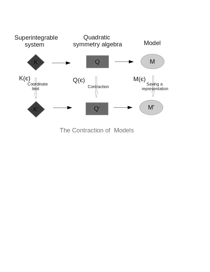
Figure 1:

8 Hypergeometric polynomials and the Askey scheme

Recall, [1], that the Wilson polynomials are defined as

$$w_{n}(t^{2})\equiv w_{n}(t^{2},a,b,c,d)=(a+b)_{n}(a+c)_{n}(a+d)_{n}\times$$ (6)

$${}_{4}F_{3}\left(\begin{array}[]{llll}-n,&a+b+c+d+n-1,&a-t,&a+t\\ a+b,&a+c,&a+d\end{array};1\right)$$

$$=(a+b)_{n}(a+c)_{n}(a+d)_{n}\Phi^{(a,b,c,d)}_{n}(t^{2}),$$

where $(a)_{n}$ is the Pochhammer symbol and ${}_{4}F_{3}(1)$ is a hypergeometric function of unit argument. The polynomial $w_{n}(t^{2})$ is symmetric in $a,b,c,d$. For the finite dimensional representations the spectrum of $t^{2}$ is $\{(a+k)^{2},\ k=0,1,\dots,m\}$ and the orthogonal basis eigenfunctions are Racah polynomials. In the infinite dimensional case they are Wilson polynomials. They are eigenfunctions for the difference operator $\tau^{*}\tau$ defined via

$$\tau = \frac{1}{2t}(E_{t}^{1/2}-E_{t}^{-1/2}),$$

$$\tau^{*} = \frac{1}{2t}\left[(a+t)(b+t)(c+t)(d+t)E_{t}^{1/2}-(a-t)(b-t)(c-t)(d-t)E_{t}^{-1/2}\right],$$

with $E_{t}^{A}F(t)=F(t+A).$

The Askey Scheme, [12, 10], organizes the theory of hypergeometric orthogonal polynomials of one variable by exhibiting the relations such that each of these polynomials can be obtained as a sequence of pointwise limits from either the Racah polynomials in the finite dimensional case or the Wilson polynomials in the infinite dimensional case.

$$\lim_{\tau\to\infty}\Phi_{n}(\tau)=\Phi^{\prime}_{n}.$$

The irreducible representations of $S9$ have a realization in terms of difference operators in 1 variable [6], exactly the structure algebra for the Wilson and Racah polynomials! By contracting these representations to obtain the representations of the quadratic symmetry algebras of the other superintegrable systems we obtain the full Askey scheme of orthogonal hypergeometric polynomials. This relationship ties the structure equations directly to physical phenomena. The full details of the contractions are given in [8]; our contribution here is to show how these contractions were induced in a natural and unique way from Lie algebra contractions which have clear physical and geometrical significance. In the following we just give some examples.

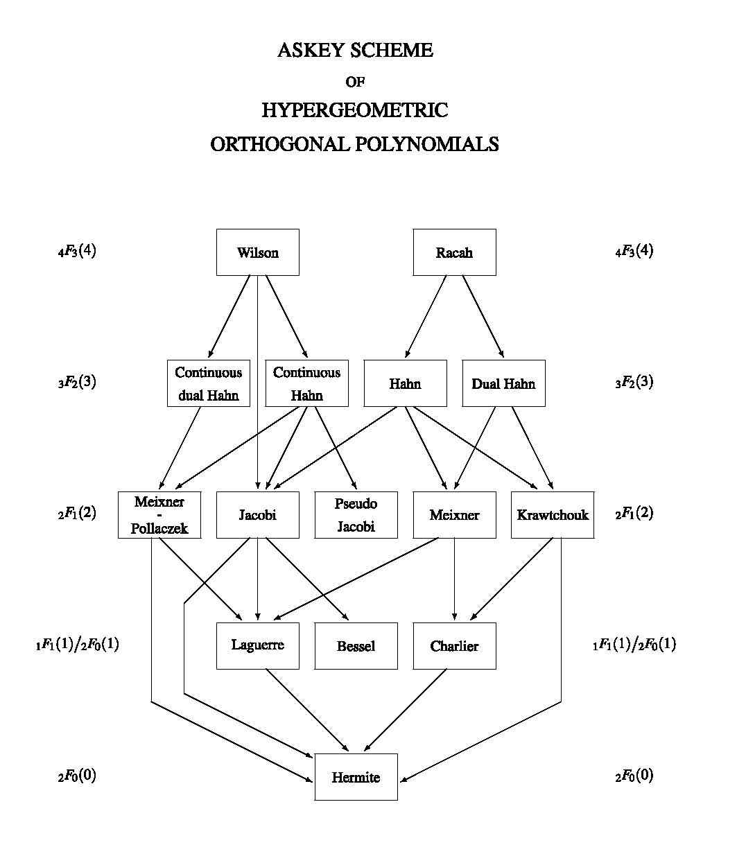
Figure 2:

9 The $S9$ difference operator model

There is no model of the irreducible representations of the quadratic algebra $S9$ in terms of differential operators but there is a difference operator model [6]:

$$L_{2}f_{n,m}=(-4t^{2}-\frac{1}{2}+B_{1}^{2}+B_{3}^{2})f_{n,m},$$

$$L_{3}f_{n,m}=(-4\tau^{*}\tau-2[B_{1}+1][B_{2}+1]+\frac{1}{2})f_{n,m},$$

$$H=L_{1}+L_{2}+L_{3}+\frac{3}{4}-(B_{1}^{2}+B_{2}^{2}+B_{3}^{2})=-4(m+1)(B_{1}+B_{2}+B_{3}+m+1)-2(B_{1}B_{2}+B_{1}B_{3}+B_{2}B_{3})$$

$$+\frac{3}{4}-(B_{1}^{2}+B_{2}^{2}+B_{3}^{2}).$$

Here $n=0,1,\cdots,m$ if $m$ is a nonnegative integer and $n=0,1,\cdots$ otherwise. Also

$$a_{j}=\frac{1}{4}-B_{j}^{2},\ \alpha=-(B_{1}+B_{3}+1)/{2}-m,\ \beta=(B_{1}+B_{3}+1)/{2},$$

$$\gamma=(B_{1}-B_{3}+1)/{2},\ \delta=(B_{1}+B_{3}-1)/{2}+B_{2}+m+2,$$

$$E^{A}F(t)=F(t+A),\ \tau=\frac{1}{2t}(E^{1/2}-E^{-1/2}),$$

$$\tau^{*}=\frac{1}{2t}\left[(\alpha+t)(\beta+t)(\gamma+t)(\delta+t)E^{1/2}-(\alpha-t)(\beta-t)(\gamma-t)(\delta-t)E^{-1/2}\right],$$

$$\ w_{n}(t^{2})=(\alpha+\beta)_{n}(\alpha+\gamma)_{n}(\alpha+\delta)_{n}{}_{4}F_{3}\left(\begin{array}[]{llll}-n,&\alpha+\beta+\gamma+\delta+n-1,&\alpha-t,&\alpha+t\\ \alpha+\beta,&\alpha+\gamma,&\alpha+\delta\end{array};1\right)$$

$$=(\alpha+\beta)_{n}(\alpha+\gamma)_{n}(\alpha+\delta)_{n}\Phi^{(\alpha,\beta,\gamma,\delta)}_{n}(t^{2}),\quad\Phi_{n}\equiv f_{n,m},$$

$$\tau^{*}\tau\Phi_{n}=n(n+\alpha+\beta+\gamma+\delta-1)\Phi_{n},$$

where $(a)_{n}$ is the Pochhammer symbol and ${}_{4}F_{3}(1)$ is a hypergeometric function of unit argument. The polynomial $w_{n}(t^{2})$ is symmetric in $\alpha,\beta,\gamma,\delta$. For the finite dimensional representations the spectrum of $t^{2}$ is $\{(\alpha+k)^{2},\ k=0,1,\cdots,m\}$ and the orthogonal basis eigenfunctions are Racah polynomials. In the infinite dimensional case they are Wilson polynomials.

The action of $L_{2}$ and $L_{3}$ on an $L_{3}$ eigenbasis is

$$L_{2}f_{n,m}=-4K(n+1,n)f_{n+1,m}-4K(n,n)f_{n,m}-4K(n-1,n)f_{n-1,m}+(B_{1}^{2}+B_{3}^{2}-\frac{1}{2})f_{n,m},$$

$$L_{3}f_{n,m}=-(4n^{2}+4n[B_{1}+B_{2}+1]+2[B_{1}+1][B_{2}+1]-\frac{1}{2})f_{n,m},$$

$$K(n+1,n)=\frac{(B_{1}+B_{2}+n+1)(n-m)(-B_{3}-m+n)(B_{2}+n+1)}{(B_{1}+B_{2}+2n+1)(B_{1}+B_{2}+2n+2)},$$

$$K(n-1,n)=\frac{n(B_{1}+n)(B_{1}+B_{2}+B_{3}+m+n+1)(B_{1}+B_{2}+m+n+1)}{(B_{1}+B_{2}+2n)(B_{1}+B_{2}+2n+1)},$$

$$K(n,n)=[\frac{B_{1}+B_{2}+2m+1}{2}]^{2}-K(n+1,n)-K(n-1,n),$$

We give an example showing how a contraction of one superintegrable system to another induces a similar contraction of models and recovers part of the Askey scheme. Our example is the contraction of $S9$ to $E1$. The full scheme of limits of orthogonal polynomials is recovered through sequences of contractions of superintegrable systems, starting from $S9$.

Quantum system limit:

$$H_{S9}=J_{1}^{2}+J_{2}^{2}+J_{3}^{2}+\frac{a_{1}}{s_{1}^{2}}+\frac{a_{2}}{s_{2}^{2}}+\frac{a_{3}}{s_{3}^{2}}$$

where $J_{3}=s_{1}\partial_{s_{2}}-s_{2}\partial_{s_{1}}$ and $J_{2},J_{3}$ are obtained by cyclic permutations of the indices $1,2,3$.

$$H_{E1}=\partial_{x}^{2}+\partial_{y}^{2}-\omega^{2}(x^{2}+y^{2})+\frac{b_{1}}{x^{2}}+\frac{b_{2}}{y^{2}}$$

In $S9$ we contract about the north pole of the unit sphere. Set

$$s_{1}=\sqrt{\epsilon}x,\ s_{2}=\sqrt{\epsilon}y,\ s_{3}=\sqrt{1-s_{1}^{2}-s_{2}^{2}}\approx 1-\frac{\epsilon}{2}(x^{2}+y^{2}),$$

$$a^{\prime}_{1}=b_{2}=a_{1},\ a^{\prime}_{2}=b_{1}=a_{2},\ a^{\prime}_{3}=-\omega^{2}=\epsilon^{2}a_{3},$$

in $H_{S9}$ to get $\epsilon({H_{S9}}-a_{3})\to{H_{E1}}$ as $\epsilon\to 0$.

Quadratic algebra contraction:

$${L}^{\prime}_{1}=\epsilon{L}_{1},\ {L}^{\prime}_{2}=\epsilon{L}_{2},\ {L}^{\prime}_{3}={L}_{3},\ {H}^{\prime}=\epsilon({H}-a_{3})$$

$${R}^{\prime}=\epsilon{R},\ a^{\prime}_{1}=b_{2}=a_{1},\ a^{\prime}_{2}=b_{1}=a_{2},\ a^{\prime}_{3}=-\omega^{2}=\epsilon^{2}a_{3}.$$

Saving a representation: We set

$$t=-x+{B_{3}}/{2}+(B_{1}+1)/{2}+m,\ B_{3}=\frac{\omega}{\epsilon}\to\infty\ \Longrightarrow$$

$$f^{\prime}_{n,m}={}_{3}F_{2}\left(\begin{array}[]{lll}-n,&B_{1}+B_{2}+n+1,&-x\\ -m,&B_{2}+1&\end{array};1\right)=Q_{n}(x;B_{2},B_{1},m)$$

where the $Q_{n}$ are Hahn polynomials. We have the model

$$L^{\prime}_{2}f^{\prime}_{n,m}=2\omega(2x-2m-B_{1}-1)f^{\prime}_{n,m}=-4K^{\prime}(n+1,n)f^{\prime}_{n+1,m}-4K^{\prime}(n,n)f^{\prime}_{n,m}-4K^{\prime}(n-1,n)f^{\prime}_{n-1,n},$$

$$L^{\prime}_{3}f^{\prime}_{n,m}=-\left(4n^{2}+4n[B_{1}+B_{2}+1]+2[B_{1}+1][B_{2}+1]-\frac{1}{2}\right)f^{\prime}_{n,m}=\qquad\qquad$$

$$\left[-4(x-m)(x+B_{2}+1)E^{1}_{x}+4x(x-m-B_{1}-1)E_{x}^{-1}+8x^{2}+4x(B_{1}+B_{2}-2m)\right.$$

$$\left.-4m(B_{2}+1)-2(B_{2}+1)(B_{1}+1)+\frac{1}{2}\right]f^{\prime}_{n,m},$$

$$H^{\prime}=L^{\prime}_{1}+L^{\prime}_{2}=-2\omega(2m+2+B_{1}+B_{2}).$$

Here the $K^{\prime}$ are the appropriate limits of the $K$ as $B_{3}\to\infty$.

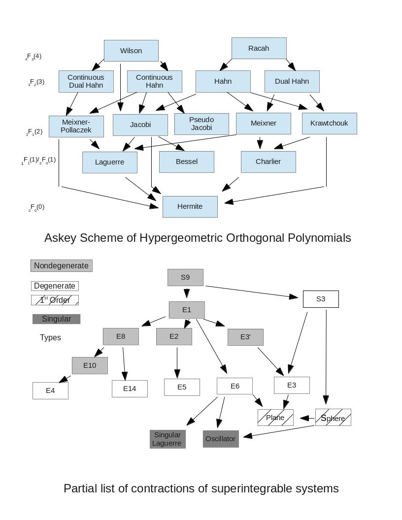
Figure 3: The Askey scheme and contractions of superintegrable systems

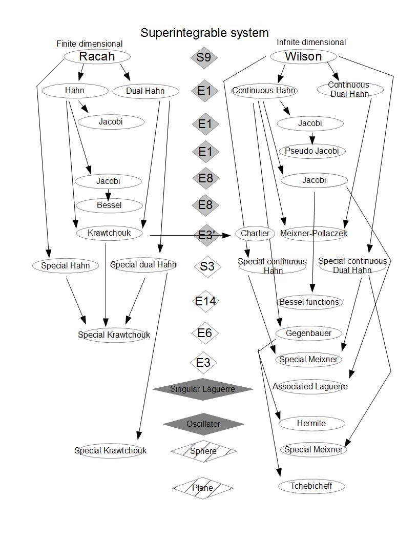
Figure 4: The Askey contraction scheme

See Figures 3 and 4 for the contraction description of the Askey Scheme.

10 Observations and conclusions

• Free quadratic algebras uniquely determine associated superintegrable systems with potential.

• A contraction of a free quadratic algebra to another uniquely determines a contraction of the associated superintegrable systems.

• For a 2D superintegrable systems on a constant curvature space these contractions can be induced by Lie algebra contractions of the underlying Lie symmetry algebra.

• Every 2D superintegrable system is obtained either as a sequence of contractions from $S9$ or is Stäckel equivalent to a system that is so obtained.

• Taking contractions step-by-step from the $S9$ model we can recover the Askey Scheme. However, the contraction method is more general. It applies to all special functions that arise from the quantum systems via separation of variables, not just polynomials of hypergeometric type, and it extends to higher dimensions [7]. The special functions arising from the models can be described as the coefficients in the expansion of one separable eigenbasis for the original quantum system in terms of another separable eigenbasis. The functions in the Askey Scheme are just those hypergeometric polynomials that arise as the expansion coefficients relating two separable eigenbases that are both of hypergeometric type. Thus, there are some contractions which do not fit in the Askey scheme since the physical system fails to have such a pair of separable eigenbases.

• The details of the Askey Scheme derivation can be found in [8]. The origin of the complicated multiparameter contractions was not clear in that paper. In this paper we have demonstrated that all of these contractions were uniquely induced by the contractions of the Lie algebras $e(2,{\bf C})$, $o(3,{\bf C})$. Details will follow in [9]. There are only a small number of these Lie algebra contractions and their action on physical space is well known.

• Even though 2nd order 2D nondegenerate superintegrable systems admit no group symmetry, their structure is determined completely by the underlying symmetry of constant curvature spaces.

• To extend the method to Askey-Wilson polynomials we would need to find appropriate $q$-quantum mechanical systems with $q$-symmetry algebras and we have not yet been able to do so.

This work was partially supported by a grant from the Simons Foundation (# 208754 to Willard Miller, Jr.).

References

References

[1] Andrews G. E., Askey, R. and Roy R.,
Special Functions. Encyclopedia of mathematics and its Applications,
Cambridge University Press, Cambridge, UK, 1999.
[2] Inönü, E. and Wigner, E. P., On the contraction of groups and their representations.
Proc. Nat. Acad. Sci. (US) (39, 510-524, (1953).
[3]A.A.Izmest’ev, G.S.Pogosyan, A.N.Sissakian, and P.Winternitz. Contractions of Lie algebras and the separation of variables , J.Phys.A, 29, 5940-5962 (1996).
[4]
Kalnins E. G., Kress J. M., Miller W. Jr. and Pogosyan G. S.,
Completeness of superintegrability in two-dimensional constant
curvature spaces.J. Phys. A: Math Gen., 2001, V.34, 4705–4720.
[5] E.G. Kalnins, W. Miller, Jr. and G.S. Pogosyan. Contractions of Lie algebras and special function identities, J. Phys. A 32,4709–4732, (1999)
[6]Kalnins E. G., Miller W. Jr and Post S., Wilson
polynomials and the generic superintegrable system on the 2-sphere,
J. Phys. A: Math. Theor.40, 11525-11538, (2007),
[7]Kalnins E. G., Miller W. Jr and Post S.
Two-variable Wilson polynomials and the generic superintegrable system on the
3-sphere, SIGMA, 7 (2011), 051, 26 pages
[8]Kalnins E. G., Miller W. Jr and Post S.
Contractions of 2D 2nd order quantum superintegrable systems and the Askey scheme for hypergeometric orthogonal polynomials,
SIGMA, 9 (2013), 057, 28 pages
[9] Kalnins E. G., Miller W. Jr., Subag E and Heinonen R.,
Contractions of 2nd order superintegrable systems in 2D. (In preparation).
(2013).
[10]
Koekoek, R., Lesky, P. A. and Swarttouw, R. F.,
(2010), Hypergeometric orthogonal polynomials and their q-analogues,
Springer Monographs in Mathematics, Berlin, New York: Springer-Verlag, 2010.
[11]
G. Koenigs. Sur les géodésiques a intégrales quadratiques. A note
appearing in “Lecons sur la théorie générale des
surfaces”. G. Darboux. Vol 4, 368-404, Chelsea Publishing 1972.
[12]
Koornwinder, T. H., (1988),
Group theoretic interpretations of Askey’s scheme of hypergeometric orthogonal polynomials,
Orthogonal polynomials and their applications (Segovia, 1986),
Lecture Notes in Math., 1329, Berlin, New York: Springer-Verlag, pp. 46–72, 1988.
[13] W Miller Jr., S. Post, and P.. Winternitz. Classical and quantum superintegrability with applications. J.
Phys. A: Math. Theor., (to appear) 2013. A 97 page review article.
[14] E. Saletan. Contractions of Lie groups.J. Math. Phys., 2, 1-21, 1961.
[15] J. Talman. Special Functions: A Group Theoretic Approach (based on the
lecture notes of Eugene Wigner) W.A. Benjamin, New York 1968.
[16] Superintegrability in Classical
and Quantum Systems,
Tempesta P., Winternitz P., Miller W., Pogosyan G., editors, AMS,
vol. 37, 2005.
[17] E. Weimar-Woods., The three-dimensional real Lie algebras and their contractions,Journal of Mathematical Physics, Volume 32, Issue 8, August 1991, pp.2028-2033.