Abstract. Jigsaw percolation is a nonlocal process that iteratively merges connected clusters in a deterministic “puzzle graph” by using connectivity properties of a random “people graph” on the same set of vertices. We presume the Erdős-Rényi people graph with edge probability $p$ and investigate the probability that the puzzle is solved, that is, that the process eventually produces a single cluster. In some generality, for puzzle graphs with $N$ vertices of degrees about $D$ (in the appropriate sense), this probability is close to 1 or small depending on whether $pD\log N$ is large or small. The one dimensional ring and two dimensional torus puzzles are studied in more detail and in many cases the exact scaling of the critical probability is obtained. The paper strengthens several results of Brummitt, Chatterjee, Dey, and Sivakoff who introduced this model.

2010 Mathematics Subject Classification: 60K35

Key words and phrases: jigsaw percolation, nucleation, random graph

1 Introduction

The two-dimensional discrete torus is the graph with vertex set $V={\mathbb{Z}}_{n}^{2}=\{0,1\dots,n-1\}^{2}$ with periodic boundary conditions and edges between nearest neighbors. We imagine $V$ as pieces of a puzzle and denote this graph, an instance of a puzzle graph, by $G_{\text{puz}}$. Suppose we have a partially solved puzzle, that is, a collection of $G_{\text{puz}}$-connected subsets of $V$ (also known as clusters) that partition $V$. Then we get closer to the complete solution by merging together one or more of these clusters. If we have two clusters whose union is a connected set in $G_{\text{puz}}$, how does the information that they fit together, and hence can be merged, get transmitted? The idea introduced in [BCDS] is that the knowledge about each piece is held by a separate person and that the $N=\left|V\right|$ people are connected by collaboration edges into the people graph $G_{\text{ppl}}$. This model was proposed as an idealized mechanism by which people with incomplete knowledge could collaboratively combine their partial solutions to solve a puzzle. As in [BCDS], we assume that people connections are sparse and assigned at random.

   

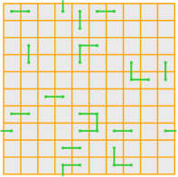
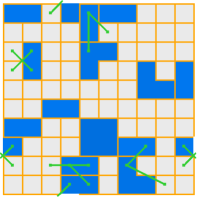
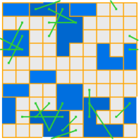
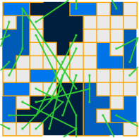
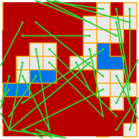
Figure 1.1: AE jigsaw percolation on $10\times 10$ torus (i.e., square with periodic boundary), with $p=0.11$, at times $t=0,\ldots,5$. The clusters are outlined in orange and colored grey-blue-dark blue-red according to their sizes. The edges of ${\mathcal{G}}_{t}$, that decide which cluster are merged in the next time step, are depicted in green. The edges connect vertices with the $G_{\text{ppl}}$-connection found by the algorithm. Clearly, all vertices are in one cluster for the first time at $t=6$.

Our general setting is a sequence of graph pairs $(G_{\text{puz}},G_{\text{ppl}})$, on a common vertex set $V$ whose size $N$ increases with an integer parameter $n$. The dependence on $n$ or $N$ is typically suppressed in our notation; $N$ will always mean the number of vertices in the graph, and for particular examples we choose the common parametrization (e.g., the two dimensional torus graph ${\mathbb{Z}}_{n}^{2}$ has $N=n^{2}$ vertices), while we formulate our statements about general graphs in terms of dependence on $N$ rather than $n$. The puzzle graph $G_{\text{puz}}=(V,E_{\text{puz}})$ is (for every $N$) a connected deterministic graph, while we assume throughout that the random people graph $G_{\text{ppl}}=(V,E_{\text{ppl}})$ is an Erdős-Rényi graph on $V$ with a small edge probability $p$ that also depends on $N$.

The models we consider retain the general flavor of [BCDS], with a new ingredient: how easy it is to discover that a puzzle piece fits to a cluster depends on the number of connections of each type between the piece and the cluster. A simple implementation of this principle leads to a three-parameter model that we now introduce.

We say that vertices $v_{1},v_{2}\in V$ are doubly connected if they are connected in both graphs: $\{v_{1},v_{2}\}\in E_{\text{ppl}}\cap E_{\text{puz}}$. For a fixed $v\in V$ and a set $S\subset V$, we let $\text{\tt coll}(v,S)$ (resp. $\text{\tt link}(v,S)$) be the number of $G_{\text{ppl}}$-neighbors (resp. $G_{\text{puz}}$-neighbors) of $v$ in $S$, not including $v$.

We define jigsaw percolation as a discrete-time dynamics with three threshold parameters: verification threshold $\sigma\geq 1$, link threshold $\tau\geq 1$, and exemption threshold $\theta\geq\tau$. At each time $t=0,1,2,\dots$, the state of the dynamics is a partition $\mathcal{P}^{t}=\{W_{i}^{t}:i=1,\dots,I_{t}\}$ of the vertex set, with $\mathcal{P}^{0}$ a given partition. Given $\mathcal{P}^{t}$, $\mathcal{P}^{t+1}$ is obtained as follows. Construct the graph ${\mathcal{G}}_{t}$ with vertex set $\mathcal{P}^{t}$ and unoriented edges between any $W_{i}^{t}$ and $W_{j}^{t}$ such that at least one of (J1)–(J3) is satisfied:

• there are doubly connected vertices $v_{1}\in W_{i}^{t}$ and $v_{2}\in W_{j}^{t}$;

• there is a vertex $v_{1}\in W_{i}^{t}$ with $\text{\tt link}(v_{1},W_{j}^{t})\geq\theta$;

• there is a vertex $v_{1}\in W_{i}^{t}$ with $\text{\tt coll}(v_{1},W_{j}^{t})\geq\sigma$ and $\text{\tt link}(v_{1},W_{j}^{t})\geq\tau$.

Then,

• to obtain $\mathcal{P}^{t+1}$, merge all sets in $\mathcal{P}^{t}$ that belong to the same connected component of ${\mathcal{G}}_{t}$.

The parameter $\theta$ is akin to the threshold in bootstrap percolation [AL], in that a vertex will merge with a larger cluster as soon as it has $\theta$ $G_{\text{puz}}$-neighbors in that cluster. In the example of ${\mathbb{Z}}_{n}^{2}$, when $\theta=2$, this amounts to filling in puzzle pieces that “obviously” fit with the partially solved puzzle because they fill in a missing corner. Of course, due to the nonlocal nature, other sites may be added to the cluster along with the missing corner (namely, those sites that have previously merged with the corner). (Another contrast with bootstrap percolation is that we get an essentially equivalent model if we require that the two neighbors, which a vertex needs in a neighboring cluster to join, are diagonally adjacent.) The parameters $\tau$ and $\sigma$ control the levels of redundancy required in the puzzle and people graphs, respectively, for two clusters to merge. We say that the event Solve happens if, when $\mathcal{P}^{0}$ consists of all singletons, the partition eventually gathers all vertices into one set, that is $\text{\tt Solve}=\{\mathcal{P}_{t}=\{V\}\text{ for some t}\}$.

Observe that, for every $t$, sets in $\mathcal{P}^{t}$ are $G_{\text{puz}}$-connected; provided that $\theta=\infty$, they are also $G_{\text{ppl}}$-connected. The model with parameters $\sigma=\tau=1$ and $\theta=\infty$ (or equivalently, $\theta$ exceeds the maximum degree of $G_{\text{puz}}$) was introduced in [BCDS] as the Adjacent-Edge (AE) jigsaw percolation and we will keep this name. The paper [BCDS] mostly analyzes the basic jigsaw percolation in which there is an edge between $W_{i}^{t}$ and $W_{j}^{t}$ in ${\mathcal{G}}^{t}$ when

• there are vertices $v_{1},v_{1}^{\prime}\in W_{i}^{t}$ and $v_{2},v_{2}^{\prime}\in W_{j}^{t}$, such that $\{v_{1},v_{2}\}\in E_{\text{ppl}}$ and $\{v_{1}^{\prime},v_{2}^{\prime}\}\in E_{\text{puz}}$.

All our results that apply to AE dynamics (Theorems 1, 2, 6, and results in Sections 3 and 4, as well as $\sigma=1$ instances of Theorems 4 and 5) hold for the basic version with unchanged proofs. In fact, as noted in [BCDS], it is an interesting open problem to devise a class of puzzle graphs with significant difference in behaviors between the AE and basic versions.

A small example of solving the torus puzzle in the AE case is depicted in Figure 1.1 and a larger one in Figure 1.2; see Section 10 for a description of algorithms we employ. The general message of simulations is that $p$ should be large enough so that nucleation centers (as in Figure 1.2) appear. In this sense, jigsaw percolation is similar to bootstrap percolation [AL, Hol] and Greenberg-Hastings model [FGG], in spite of the fact that it is non-local. Indeed, to our knowledge the present paper is the first to establish scaling of critical probabilities and sharp phase transitions using nucleation techniques in a non-local setting.

Typical for nucleation-and-growth models is an order parameter: a function of $p$ and $N$ that determines (for large $N$) whether $\mathbb{P}_{p}\left(\text{\tt Solve}\right)$ is large or small; often there is sharp transition from probability close to $0$ to close to $1$. For example, we will prove that for the ${\mathbb{Z}}^{2}_{n}$ case of Figure 1.1, the order parameter is $p\log n$, but a sharp transition in this case remains an open problem. To make this concept precise, we define the critical probability $p_{c}=p_{c}(N)$ by

$$\mathbb{P}_{p_{c}}\left(\text{\tt Solve}\right)=\frac{1}{2}.$$

We say that there is sharp transition if $\mathbb{P}_{(1-\epsilon)p_{c}}\left(\text{\tt Solve}\right)\to 0$ and $\mathbb{P}_{(1+\epsilon)p_{c}}\left(\text{\tt Solve}\right)\to 1$ as $N\to\infty$, for any $\epsilon>0$. It is expected that under general conditions there is sharp transition [FK]. We will prove this for some examples in which the asymptotic behavior of $p_{c}$ can be determined exactly. The general results in [FK] (and subsequent work) cannot be used as they depend on symmetry of random bits. This in our case clearly fails as, for example, $G_{\text{ppl}}$-edges between $G_{\text{puz}}$-neighbors do not play exactly the same role as other $G_{\text{ppl}}$-edges. We refer to [BCDS] for much more background and intuition. We now state our main results, which are divided into three categories in subsections below.

1.1 Results for general puzzle graphs

Notably, the asymptotic order of $p_{c}$ can be determined in some generality. In this subsection, we assume the puzzle graph $G_{\text{puz}}$ has maximum degree $D$, which may depend on $N$. The proof of the following theorem is given in Section 3.

Theorem 1.

Assume AE dynamics and that $p=\mu/(D\log N)$ for a constant $\mu\leq 1/30$. Then $\mathbb{P}_{p}\left(\text{\tt Solve}\right)\to 0$.

Theorem 2 from [BCDS] demonstrates that for the AE dynamics $\mathbb{P}_{p}\left(\text{\tt Solve}\right)\to 1$ if $p\geq C/\log N$, for an absolute constant $C$. The next theorem provides a more precise result for some well-known vertex-transitive graphs: together with Theorem 1 it implies that $p_{c}$ scales as $1/(D\log N)$ in these cases. On the other hand, in Section 4 we will exhibit a vertex-transitive example for which this scaling does not hold. Section 4 also contains a general method used to prove results such as Theorem 2.

Theorem 2.

Assume AE dynamics and $p=\mu/(D\log N)$ for a constant $\mu$. For each of the following vertex-transitive graphs, there exists a universal constant $C$ such that $\mu\geq C$ implies $\mathbb{P}_{p}\left(\text{\tt Solve}\right)\to 1$: $d$-dimensional torus ${\mathbb{Z}}_{n}^{d}$ with lattice edges; range-$r$ two-dimensional graph on ${\mathbb{Z}}_{n}^{2}$ with neighborhood of $x$ given by $\{y:||x-y||_{\infty}\leq r\}$; hypercube with vertex set $\{0,1\}^{n}$; and $d$-dimensional Hamming graph with vertex set ${\mathbb{Z}}_{n}^{d}$.

An important question we attempt to answer in various contexts is the following: how costly is it to require a large number of verifications in the people graph? Our next result, proved in Section 6, clarifies the general answer for the most natural setting whereby we keep the AE parameters $\tau=1$, $\theta=\infty$, but assume $\sigma$ is large. It turns out that the number of people connections required to solve the puzzle then increases as the square of $\sigma$.

Theorem 3.

Assume that $\tau=1$, $\theta=\infty$, and $\sigma$ is arbitrary. Assume also that the degree $D$ is bounded by a constant independent of $N$. Then, for $N\geq N_{0}(\sigma)$, $p_{c}$ is between two constants times $\sigma^{2}/\log N$.

1.2 Results for the ring graph

We next turn to more precise results for low-dimensional puzzle lattices. As pointed out in [BCDS], the one-dimensional ring puzzle with $V={\mathbb{Z}}_{n}$ is already of interest. By exploiting remarkable similarity to two-dimensional bootstrap percolation (see Section 5 for details), we prove Conjecture 2 of [BCDS] and shed light on Open Problem 1 in the same paper. For $\sigma\geq 1$, we let

$$g_{\sigma}(x)=-\log\mathbb{P}\left({\mathrm{Poisson}}(x)\geq\sigma\right)$$

and

$$\lambda_{\sigma}=\int_{0}^{\infty}g_{\sigma}(x)\,dx.$$

Theorem 4.

Assume the ring puzzle graph with $\tau=1$, $\theta=\infty$, and arbitrary $\sigma\geq 1$. As $n\to\infty$,

$$p_{c}\log n\to\lambda_{\sigma},$$

with sharp transition.

Theorem 5.

In the context of Theorem 4, assume $p\sim\lambda/\log n$, for some $\lambda>0$. Let $T_{f}=\min\{t:\mathcal{P}_{t+1}=\mathcal{P}_{t}\}$ be the time when the jigsaw dynamics stops. Then, in probability,

$$\begin{cases}\limsup_{n\to\infty}\frac{T_{f}}{\log n}<\infty&\text{if $\lambda<\lambda_{\sigma}$}\\ \lim_{n\to\infty}\frac{\log T_{f}}{\log n}=\frac{\lambda_{\sigma}}{\lambda}&\text{if $\lambda>\lambda_{\sigma}$}\end{cases}$$

Roughly then, for large $n$, $(\log n)^{-1}\log T_{f}$ as a function of $p\log n$ vanishes on $[0,\lambda_{\sigma})$, has a discontinuous jump to $1$ at $\lambda_{\sigma}$ and then decreases to 0 as the inverse first power. For a comparison with simulations, see Figure 5b in [BCDS].

1.3 Results for the two dimensional torus

The bulk of the paper is devoted to the case of two-dimensional lattice torus $G_{\text{puz}}$ with $V={\mathbb{Z}}_{n}^{2}$, which will be assumed in Theorems 6, 7, and 8. We begin with the AE dynamics, for which Theorems 1 and 2 imply that the order parameter is $p\log n$, as previously announced. While we are unable to prove sharp transition, we will at least give upper and lower bounds within a factor of $10$. We suspect the lower bound is the cruder of the two; see Section 7 for a proof.

Theorem 6.

Assume the AE dynamics. For a large enough $n$,

$$\frac{0.0388}{\log n}<p_{c}<\frac{0.303}{\log n}.$$

The two-dimensional torus is the simplest instance for which we can investigate the dependence on two puzzle graph thresholds $\theta$ and $\tau$. It it is not hard to see that for this $G_{\text{puz}}$ there are essentially only three interesting cases: $\tau=1,\theta=\infty$; $\tau=1$, $\theta=2$; and $\theta\geq\tau=2$. The first case is covered by Theorems 6 and 3, while the other two are addressed in our next two results. Many open problems remain for other puzzle graphs; see the Open problems section at the end of the paper.

Our most substantial result is about the parameter choice $\tau=1$ and $\theta=2$. In this case, corners are fit automatically, but non-corner pieces require $\sigma\geq 1$ verifications. By contrast to Theorem 3, and perhaps surprisingly, $\sigma$ now affects the power of $\log n$ in the critical scaling. Change of the order parameter without a change in the underlying geometry appears to be a novel phenomenon. We let $g(x)=g_{1}(x)=-\log(1-e^{-x})$ and

$$\nu_{\sigma}=\int_{0}^{\infty}g\left(\frac{x^{2\sigma+1}}{\sigma!}\right)\,dx=\frac{(\sigma!)^{1/(2\sigma+1)}\Gamma(\frac{1}{2\sigma+1})\zeta(\frac{2\sigma+2}{2\sigma+1})}{2\sigma+1}.$$

For example, when $\sigma=1$, $\nu_{1}=\frac{\Gamma(\frac{1}{3})\zeta(\frac{4}{3})}{3}\approx 3.216$ and the next theorem implies that transition occurs at $p(\log n)^{3}=\nu_{1}^{3}\approx 33.25$. See Figure 1.2 for an illustration and Section 8 for a proof.

Theorem 7.

Assume $\tau=1$, $\theta=2$ and $\sigma\geq 1$. As $n\to\infty$,

$$p_{c}(\log n)^{2+\frac{1}{\sigma}}\to\nu_{\sigma}^{2+\frac{1}{\sigma}},$$

with sharp transition.

The final interesting case has $\tau=2$, and arbitrary $\theta$ and $\sigma$. The asymptotic scaling of the critical probability is always $1/\log n$, but the only instance we are able to identify the constant factor is when $\theta=2$ and the dynamics does not depend on $\sigma$. We give a proof in Section 9 and, again, Figure 1.2 provides an illustration.

Theorem 8.

Assume $\theta\geq\tau=2$, and $\sigma\geq 1$. Then,

(1.1) $$\frac{\pi^{2}}{6}\leq\liminf_{n\to\infty}p_{c}\log n\leq\limsup_{n\to\infty}p_{c}\log n\leq\frac{\pi^{2}}{6}+\frac{1}{2}\int_{0}^{\infty}g_{\sigma}(x)\,dx.$$

If $\tau=\theta=2$, then

(1.2) $$p_{c}\sim\frac{\pi^{2}}{6}\cdot\frac{1}{\log n}$$

as $n\to\infty$, with sharp transition.

The lower bound in (1.1) can be improved for large $\sigma$, as Theorem 3 implies that it can be replaced by a bound on the order $\sigma^{2}$. We do not know whether the upper bound in (1.1) (which is also on the order $\sigma^{2}$) can be improved.

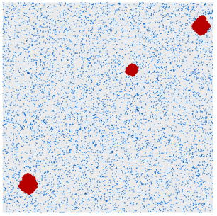
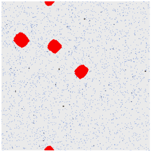
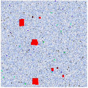
Figure 1.2: Jigsaw percolation on $400\times 400$ torus. Top left: AE version ($\sigma=\tau=1$, $\theta=\infty$) with $p=0.021$, at time $t=31$. Top right: $\sigma=\tau=1$, $\theta=2$ with $p=0.009$, at $t=31$. Bottom: $\sigma=1$, $\tau=2$, $\theta=\infty$, with $p=0.11$ at $t=91$. These pictures illustrate the nucleation and metastability of the dynamics: most of the space is divided into small clusters (color-coded by size with grey singletons). A few favorable local configurations generate large (red) clusters that grow unstoppably and result in Solve.

We remark that for random puzzle graphs, a related result was proven in [Sli], where it is assumed that both the people and puzzle graphs are Erdős-Rényi with probabilities $p$ and $p_{\text{puz}}$, respectively, with $p\wedge p_{\text{puz}}\geq(1+\epsilon)\log N/N$ for some $\epsilon>0$. Then it is shown that the probability of solving the puzzle is close to zero if $p\cdot p_{\text{puz}}\leq c/(N\log N)$ and is close to one if $p\cdot p_{\text{puz}}\geq C\log\log N/(N\log N)$, for some constants $c,C>0$.

The rest of the paper is organized as follows. We begin with Section 2 that contains more formal definitions and some useful observations. Sections 3–9 are devoted to proofs to the above theorems. Section 10 contains a discussion of computational aspects of simulation algorithms, and the paper is concluded by a list of intriguing open problems.

2 Preliminaries

We say that a given partition $\mathcal{P}$ is inert if jigsaw percolation started at $\mathcal{P}^{0}=\mathcal{P}$ results in ${\mathcal{G}}^{0}$ with no edges and thus $\mathcal{P}^{1}=\mathcal{P}$. Clearly, for any $\mathcal{P}^{0}$, $\mathcal{P}^{t}$ is inert for some $t$; we call this the final partition started from $\mathcal{P}_{0}$. Note that the final partition also depends on $G_{\text{ppl}}$.

When not explicitly stated otherwise, the initial partition $\mathcal{P}^{0}$ will consist of all singletons and in this case we denote the final partition as final.

For a given set $S\subset V$, denote its outside boundary by $\partial_{o}(S)=\{v\notin S:\{v,v^{\prime}\}\in E_{\text{puz}}\text{ for some }v^{\prime}\in S\}$.

Proposition 2.1.

Assume that $\{\mathcal{P}_{j}\}$ is a finite collection of inert partitions of $V$, and let the partition $\mathcal{P}$ consist of all non-empty intersections $\cap_{j}W_{j}$ for arbitrary $W_{j}\in\mathcal{P}_{j}$. Then $\mathcal{P}$ is also inert.

Proof.

A partition $\mathcal{P}$ is inert if and only if for every $W\in\mathcal{P}$ and every vertex $v\in\partial_{o}(W)$ all of the following hold: $v$ is not doubly connected to any vertex in $W$; $\text{\tt link}(v,W)<\theta$; $\text{\tt coll}(v,W)<\sigma$ or $\text{\tt link}(v,W)<\tau$. To show this holds for the so defined $\mathcal{P}$, pick $v\in\partial_{o}(\cap_{j}W_{j})$ for arbitrary $W_{j}\in\mathcal{P}_{j}$ such that their intersection is nonempty. Then $v\in\partial_{o}(W_{j_{0}})$ for some $j_{0}$ and $\text{\tt link}(v,\cap_{j}W_{j})\leq\text{\tt link}(v,W_{j_{0}})<\theta$. Other verifications are similar. ∎

By Proposition 2.1, for any partition $\mathcal{P}^{0}$, there exists an inert partition $\langle\mathcal{P}^{0}\rangle$, which is the finest of all inert partitions $\mathcal{P}$ such that $\mathcal{P}^{0}$ is finer than $\mathcal{P}$.

We call a dynamics on partitions a slowed-down jigsaw percolation if (J4) is replaced by the following.

• If ${\mathcal{G}}_{t}$ has no edges, $\mathcal{P}^{t+1}=\mathcal{P}^{t}$; otherwise use some rule to choose any nonempty subset of edges of ${\mathcal{G}}_{t}$ to form a graph ${\mathcal{G}}_{t}^{\prime}$, then merge all sets in $\mathcal{P}^{t}$ which are in the same connected component of ${\mathcal{G}}_{t}^{\prime}$ to obtain $\mathcal{P}^{t+1}$.

The following corollary, which is now immediate, in particular states that the final partition is independent of the slowed-down version.

Corollary 2.2.

For any slowed-down jigsaw percolation, and any $\mathcal{P}^{0}$, there exists a $t$ for which $\mathcal{P}^{t}=\langle\mathcal{P}^{0}\rangle$.

We recall that, for a given graph $G_{\text{puz}}$ and a choice of parameters $\sigma$, $\tau$, and $\theta$, we let Solve be the event $\{\text{\tt final}=\{V\}\}$ that the jigsaw percolation eventually gathers all vertices in a single cluster. (Recall also that the random partition final assumes the default partition $\mathcal{P}^{0}$ that consists of singletons.) Most of this paper will be concerned with estimating $\mathbb{P}_{p}\left(\text{\tt Solve}\right)$ for particular choices of $p$. Figure 1.2 and analogy with other nucleation processes [AL, Hol, GH, GHM, FGG], suggest that the dominant mechanism in jigsaw percolation is growth from a single center into undisturbed environment. This approach yields a good, and often optimal, lower bound on the probability of Solve, as we will see. Thus we introduce the following local jigsaw percolation. As before, we assume that $G_{\text{puz}}$ is a connected deterministic graph on $V$ and $G_{\text{ppl}}$ is a random graph in which each pair of vertices is independently connected with a probability $p$, but here $V$ is typically infinite. Fix a center $v_{0}\in V$. The dynamics iteratively determines random sets $V_{0}\subset V_{1}\subset\ldots\subset V$. Let $V_{0}=\{v_{0}\}$. For $t\geq 0$, $V_{t+1}\supset V_{t}$ is obtained by adjoining to $V_{t}$ any $z\in V$ which is either: doubly connected to a point in $V_{t}$; or $\text{\tt link}(z,V_{t})\geq\theta$; or ($\text{\tt link}(z,V_{t})\geq\tau$ and $\text{\tt coll}(z,V_{t})\geq\sigma$). Define the event

$$\text{\tt Grow}=\{\cup_{t}V_{t}=V\}.$$

We will use comparison with the local version when $G_{\text{puz}}$ is the two-dimensional torus ${\mathbb{Z}}_{n}^{2}$. In this case, the corresponding local process is on the first quadrant ${\mathbb{Z}}_{+}^{2}$ with center $(0,0)$. As we will see, $\mathbb{P}_{p}\left(\text{\tt Solve}\right)\approx n^{2}\mathbb{P}_{p}\left(\text{\tt Grow}\right)$ in the relevant regime.

For a graph $G=(V,E)$ and a subset of vertices, $A\subset V$, let $G^{A}$ denote the subgraph of $G$ induced by $A$. That is, $G^{A}$ is the graph with vertex set $A$ and edge set $E^{A}=\{\{u,v\}\in E:u,v\in A\}$.

We say that a subset of vertices, $A\subset V$, is internally solved [BCDS] if the jigsaw percolation process with people graph $G_{\text{ppl}}^{A}$ solves the puzzle graph $G_{\text{puz}}^{A}$. We denote this event as $\text{\tt Solve}_{A}$. Similarly, for a partition $\mathcal{P}^{0}$ of $A$, we denote by $\langle\mathcal{P}^{0}\rangle_{A}$ the final partition obtained by running the jigsaw percolation with the two induced graphs, and let $\text{\tt final}_{A}=\langle\mathcal{P}^{0}\rangle_{A}$ when $\mathcal{P}^{0}$ is the set of singletons of $A$.

For two sets $A\subset A^{\prime}\subset V$, we let $D(A,A^{\prime})$ be the event that $\langle\mathcal{P}^{0}\rangle_{A^{\prime}}=\{A^{\prime}\}$ when the initial partition is $\mathcal{P}^{0}=\{A,\{v\}:v\in A^{\prime}\setminus A\}$. Therefore,

$$\mathbb{P}_{p}\left(\text{\tt Solve}_{A^{\prime}}\mid\text{\tt Solve}_{A}\right)=\mathbb{P}_{p}\left(D(A,A^{\prime})\right),$$

and we may think of $D(A,A^{\prime})$ as the event that jigsaw percolation internally solves $A^{\prime}$ provided it has already solved $A$.

We now state a key observation; see [AL] for the analogous result for bootstrap percolation.

Lemma 2.3.

For any slowed-down jigsaw percolation, all sets in the partition at any time are internally solved. If Solve happens, then for any $k\leq N/2$ there exists an $A\subset V$, with $|A|\in[k,2k]$, such that $\text{\tt Solve}_{A}$ happens.

Proof.

The first claim is a simple observation. For the second claim, consider a slowed-down jigsaw percolation where at each step the graph ${\mathcal{G}}_{t}^{\prime}$ in (J6) has at most one edge, so that if the process does not stop exactly two clusters merge. In this version, the size of the largest cluster can at most double in a single step. ∎

We call a set $A\subset V$ of vertices unstoppable if every vertex $v\in V\setminus A$ is $G_{\text{ppl}}$-connected to at least $\sigma$ vertices in $A$. The following simple observation is frequently used.

Lemma 2.4.

Assume $\tau=1$. For any $A\subset V$,

$$\text{\tt Solve}_{A}\cap\{A\text{ is unstoppable}\}\subset\text{\tt Solve}.$$

Lemma 2.5.

Assume that $S\subset V$ is a set of size at least $\alpha\frac{\log N}{p}$, for $\alpha>\sigma$. Then,

$$\mathbb{P}_{p}\left(\text{$S$ is unstoppable}\right)\geq 1-3\sigma N^{1-\alpha/\sigma}.$$

Proof.

If $|S|=k$,

(2.1) $$\mathbb{P}_{p}\left(\text{$S$ is not unstoppable}\right) \leq(N-k)(1-\mathbb{P}\left(\text{\rm Binomial}(k,p)\geq\sigma\right))$$

$$\leq N(1-\mathbb{P}\left(\text{\rm Binomial}(\lfloor k/\sigma\rfloor,p)\geq 1\right)^{\sigma})$$

$$=N(1-(1-(1-p)^{\lfloor k/\sigma\rfloor})^{\sigma})$$

$$\leq N(1-(1-e^{-p\lfloor k/\sigma\rfloor})^{\sigma})$$

$$\leq\sigma Ne^{-p\lfloor k/\sigma\rfloor}.$$

∎

Another useful simple observation concerns “dividing up” the edge probability in $G_{\text{ppl}}$.

Lemma 2.6.

If $p_{j}\geq 0$, then the union of independent $G_{\text{ppl}}$-graphs with edge probabilities $p_{j}$ is stochastically dominated by the $G_{\text{ppl}}$-graph with edge probability $1\wedge\sum_{j}p_{j}$.

The following elementary lemma is useful when estimating large deviation probabilities of a binomial random variable with small expectation.

Lemma 2.7.

For all $m$, $k$, $\beta$,

(2.2) $$\mathbb{P}\left(\text{\rm Binomial}(m,\beta)\geq k)\right)\leq\binom{m}{k}\beta^{k}\leq\left(\frac{3m\beta}{k}\right)^{k}.$$

In Section 4, we also need the following large deviation bound.

Lemma 2.8.

If $p$ is small enough, $P(\text{\rm Binomial}(n,p)\leq np/2)\leq\exp(-np/7)$.

If we have an event $A$ (that depends on $N$), and $\mathbb{P}_{p}\left(A\right)\to 1$ as $N\to\infty$, we say that $A$ occurs asymptotically almost surely (a. a. s.).

Finally, we remark that we often omit integer parts when we specify integer quantities such as lengths and rectangle dimensions.

3 General graphs: lower bound

Assume the puzzle graph $G_{\text{puz}}$ has maximum degree $D$, which may depend on $\left|V\right|=N$. We will prove the following result, which implies Theorem 1. We assume the AE dynamics, that is, parameters $\tau=\sigma=1$, $\theta=\infty$, throughout this section.

Theorem 3.1.

If $p=\mu/(D\log N)$ and $\mu<\min\{2e^{-(3+\eta)},e^{-(5+\eta)/2}\}$ where $\eta=\limsup\frac{\log D}{\log N}$, then $\mathbb{P}_{p}\left(\text{\tt Solve}\right)\to 0$.

Remark 3.2.

Notice that $\eta\in[0,1]$, and the two expressions in the constraint on $\mu$ are equal when $\eta=2\log 2-1$.

When combined with Theorem 2 of [BCDS], Theorem 3.1 gives the following corollary.

Corollary 3.3.

If $G_{\text{puz}}$ has maximum degree bounded above by $D$ as $N\to\infty$, then $p_{c}$ is bounded between two constants (depending only on $D$) times $1/\log N$.

The proof of the Theorem 3.1 appears after the next two important lemmas.

Lemma 3.4.

Suppose $A\subset V$ is a set of vertices such that $\left|A\right|=\alpha\log N$ and $G_{\text{puz}}^{A}$ is connected. If $p=\mu/(D\log N)$ with $\mu<2D/\alpha$, then

$$\mathbb{P}_{p}\left(\text{\tt Solve}_{A}\right)\leq\frac{2D}{\alpha\mu}N^{\alpha(1-\alpha\mu/(2D)-\log(\frac{2D}{\alpha\mu}))}.$$

Proof.

Observe that in order to solve any connected puzzle, the people graph must at least be connected, and any connected graph on $\left|A\right|$ vertices must have at least $\left|A\right|-1$ edges, so

(3.1) $$\mathbb{P}_{p}\left(\text{\tt Solve}_{A}\right)\leq\mathbb{P}_{p}\left(G_{\text{ppl}}^{A}\text{ is connected}\right)\leq\mathbb{P}_{p}\left(\left|E_{\text{ppl}}^{A}\right|\geq\left|A\right|-1\right).$$

The distribution of $\left|E_{\text{ppl}}^{A}\right|$ is stochastically dominated by Binomial($\left|A\right|^{2}/2,p$), so for any $\theta>0$ we have

$$\mathbb{P}_{p}\left(\left|E_{\text{ppl}}^{A}\right|\geq\left|A\right|-1\right) =\mathbb{P}_{p}\left(e^{\theta\left|E_{\text{ppl}}^{A}\right|}\geq e^{\theta(\left|A\right|-1)}\right)$$

$$\leq e^{-\theta(\left|A\right|-1)}\left[1+\left(e^{\theta}-1\right)p\right]^{\left|A\right|^{2}/2}$$

$$\leq\exp\left[(e^{\theta}-1)\left|A\right|^{2}p/2-\theta\left|A\right|+\theta\right].$$

Substituting $\theta=\log(2D/(\alpha\mu))>0$, and using inequality (3.1) gives the result. ∎

Lemma 3.5.

Fix a vertex $v\in V$, and let

$$C(v,k):=\{A\subset V:v\in A,\left|A\right|=k,G_{\text{puz}}^{A}\text{ is connected}\}.$$

Then,

$$\left|C(v,k)\right|\leq(eD)^{k}$$

The proof follows an argument of Kesten ([Kes1], pg. 85).

Proof.

Consider independent site percolation on $G_{\text{puz}}$ with vertex probability $1/D$. The probability that $A$ is a connected component in the site percolation graph is

$$(1/D)^{k}(1-1/D)^{\left|\partial_{o}A\right|}\geq(1/D)^{k}(1-1/D)^{(D-1)k},$$

where the inequality follows because every vertex in $A$ has at most $D$ neighbors, at least one of which is in $A$. Summing the probability that $A$ is a connected component in the site percolation graph over all sets $A\in C(v,k)$ gives the probability that $v$ is in a site percolation cluster of size $k$, which of course is at most $1$. Therefore,

$$\left|C(v,k)\right|(1/D)^{k}(1-1/D)^{(D-1)k}=\sum_{A\in C(v,k)}(1/D)^{k}(1-1/D)^{(D-1)k}\leq 1.$$

This yields

$$\left|C(v,k)\right| \leq[D(1-1/D)^{-D+1}]^{k}=D^{k}\left[1+\frac{1}{D-1}\right]^{(D-1)k}\leq D^{k}e^{k},$$

where in the last inequality we used $1+x\leq e^{x}$. ∎

Proof of Theorem 3.1.

Apply Lemma 2.3 with $k=\log N$, then apply Lemmas 3.4 and 3.5 to get

$$\mathbb{P}_{p}\left(\text{\tt Solve}\right) \leq\mathbb{P}_{p}\left(\bigcup_{A\subset V:\left|A\right|\in[\log N,2\log N]}\text{\tt Solve}_{A}\right)$$

$$\leq\sum_{v\in V}\sum_{k\in[\log N,2\log N]}\sum_{A\in C(v,k)}\mathbb{P}_{p}\left(\text{\tt Solve}_{A}\right)$$

$$\leq(N\log N)\cdot\sup_{\alpha\in[1,2]}\left\{(eD)^{\alpha\log N}\frac{2D}{\alpha\mu}N^{\alpha(1-\alpha\mu/(2D)-\log(\frac{2D}{\alpha\mu}))}\right\}$$

$$\leq\frac{2}{\mu}(\log N)\sup_{\alpha\in[1,2]}\exp\left[\left(2\alpha+1+\frac{\log D}{\log N}-\alpha^{2}\mu/(2D)-\alpha\log\left(\frac{2}{\alpha\mu}\right)\right)\log N\right].$$

When the $\limsup$ of the coefficient of $\log N$ in the exponential is strictly smaller than $0$ for any $\alpha\in[1,2]$, we see that $\mathbb{P}_{p}\left(\text{\tt Solve}\right)\to 0$. Recalling that $\eta=\limsup(\log D/\log N)$, this condition is satisfied whenever

$$\mu <2e^{-2}\inf_{\alpha\in[1,2]}\frac{1}{\alpha}e^{-(1+\eta)/\alpha}$$

$$=2e^{-2}\min\left\{e^{-(1+\eta)},\frac{1}{2}e^{-(1+\eta)/2}\right\}.$$

This completes the proof. ∎

4 General graphs: upper bound

We first formulate a general theorem, then prove Theorem 2 in subsequent corollaries. This section is also devoted only to AE dynamics.

Fix a graph $G=(V,E)$, and positive integers $a$ and $k$. We will denote by $\mathcal{S}_{k}$ a set of sequences of length $k$, consisting of vertices and started at a fixed vertex $v_{0}\in V$. We will assume that $\mathcal{S}_{k}$ is given recursively by a building algorithm as follows. Let $\mathcal{S}_{0}=\{v_{0}\}$. For every $i\in[1,k]$, there exists a a successor map $\text{\tt Step}_{i}$ defined on $\mathcal{S}_{i-1}$ that attaches to every sequence $(v_{0},\ldots,v_{i-1})\in\mathcal{S}_{i-1}$ a set $\text{\tt Step}_{i}(v_{0},\ldots,v_{i-1})\subset V$, so that

$$\mathcal{S}_{i}=\{(v_{0},\ldots,v_{i-1},v_{i}):(v_{0},\ldots,v_{i-1})\in\mathcal{S}_{i-1},v_{i}\in\text{\tt Step}_{i}(v_{0},\ldots,v_{i-1})\}.$$

We also assume that each $B=\text{\tt Step}_{i}(v_{0},\ldots,v_{i-1})\subset V$ is ordered, and for $w\in B$, we let $\overleftarrow{B}^{w}$ be the set of vertices in $B$ that are ahead of, or equal to, $w$ in the ordering. We think of $\overleftarrow{B}^{v_{i}}$ as the “inspected” vertices. We call $\mathcal{S}_{k}$ $a$-admissible if the following holds. Fix any sequence $(v_{0},\ldots,v_{k})\in\mathcal{S}_{k}$, and let $B_{i}=\text{\tt Step}_{i}(v_{0},\ldots,v_{i-1})$, $1\leq i\leq k$, and $B_{0}=\{v_{0}\}$. Then, for $1\leq i\leq k$,

• $|B_{i}|\geq a$;

• $\{v_{0},\ldots,v_{i}\}$ is a connected subset of graph $G$; and

• The selection up to $i$ does not affect selection at $i$, i.e.,

  (4.1) $$\left(\bigcup_{j=0}^{i-1}\overleftarrow{B}_{j}^{v_{j}}\right)\bigcap B_{i}=\emptyset.$$

For a fixed probability $q$, we call ${\text{\tt Size}}(G,v,q)$ the (random) number of vertices in the connected component of $v\in V$ in site percolation on $G$ where vertices other than $v$ are open independently with probability $q$, and $v$ is open with probability $1$.

For a nondecreasing integer sequence $D_{N}$, we call a sequence of $G_{\text{puz}}$-graphs $D_{N}$-regular if the following is true for some constants $c,C>0$: $D_{N}\geq 2C$ and there exist disjoint sets $V_{\ell}\subset V$, $\ell=1,\ldots,N^{c}$, so that induced subgraphs $G_{\ell}=G_{\text{puz}}^{V_{\ell}}$ have the properties that

• for each $\ell=1,\ldots,N^{c}$, $G_{\ell}$ contains a $cD_{N}$-admissible set of length at least $c\log N$ started at some $w_{\ell}\in V_{\ell}$; and

• $\liminf_{N}\inf_{\ell}\mathbb{P}\left({\text{\tt Size}}(G_{\ell},w_{\ell},C/D_{N})\geq 2D_{N}(\log N)^{2}\right)>0$.

Theorem 4.1.

If $G_{\text{puz}}$ is $D_{N}$-regular, and $p=\frac{\mu}{D_{N}\log N}$ for a large enough constant $\mu$, then $\mathbb{P}_{p}\left(\text{\tt Solve}\right)\to 1$.

Proof.

We will use Lemma 2.6, with three probabilities. Assume first that $p_{1}=\mu_{1}/(D_{N}\log N)$, where $\mu_{1}=3/c^{2}$. Fix an $\ell$ and let $F_{1}$ be the event that $w_{\ell}$ is included in an internally solved set of size $c\log N$ within $G_{\ell}$. By (R1), we may build such a cluster by using the building algorithm for the $cD_{N}$-admissible set of sequences. In this algorithm, we let $v_{0}=w_{\ell}$ and check the vertices in $\text{\tt Step}_{i}(v_{0},\ldots,v_{i-1})$ in their given order and stop checking once we find one that is $G_{\text{ppl}}$-connected to $\{v_{0},\ldots,v_{i-1}\}$. Therefore,

(4.2) $$\mathbb{P}_{p_{1}}\left(F_{1}\right) \geq\prod_{i=1}^{c\log N}\left(1-(1-p_{1})^{cD_{N}i}\right)$$

$$\geq\prod_{i=1}^{\infty}\left(1-e^{-p_{1}cD_{N}i}\right)$$

$$\geq\exp\left(\int_{0}^{\infty}\log(1-e^{-p_{1}cD_{N}x})\,dx\right)$$

$$=\exp\left(-\frac{\pi^{2}}{6c}\cdot\frac{1}{p_{1}D_{N}}\right)$$

$$=N^{-\frac{\pi^{2}}{6c\mu_{1}}}.$$

Now assume that $p_{2}=\mu_{2}/(D_{N}\log N)$, for $\mu_{2}=2C/c$. Connect each pair of vertices with a green edge independently with probability $p_{2}$. Then declare each vertex in $V_{\ell}$ to be open if it has a green edge to at least one of the vertices in the largest internally solved subset of $V_{\ell}$ containing $w_{\ell}$ in the independent people graph with the $G_{\text{ppl}}$-edge probability $p_{1}$. If $F_{1}$ happens, the probability that a vertex is open is, since $C/D_{N}\leq 0.5$, at least $C/D_{N}$ independently of other vertices, and (R2) applies. Let $F_{2}$ be the event that $w_{\ell}$ is included in an internally solved set within $G_{\ell}$ of size $2D_{N}(\log N)^{2}$. By (R2), (4.2) and Lemma 2.6,

(4.3) $$\mathbb{P}_{p_{1}+p_{2}}\left(F_{2}\right)\geq\alpha N^{-\frac{\pi^{2}}{6c\mu_{1}}},$$

for some constant $\alpha>0$. Therefore, by (R1) and (4.3),

(4.4) $$\mathbb{P}_{p_{1}+p_{2}}\left(\text{there is an internally solved set of size $2D_{N}(\log N)^{2}$}\right)$$

$$\geq 1-\left(1-\alpha N^{-\frac{\pi^{2}}{6c\mu_{1}}}\right)^{N^{c}}$$

$$\geq 1-\exp(-\alpha N^{c-\frac{2}{c\mu_{1}}})$$

$$=1-\exp(-\alpha N^{c/3}).$$

Now let $p_{3}=1/(D_{N}\log N)$. If a fixed set $V_{0}$ of vertices has size at least $2D_{N}(\log N)^{2}$, then by Lemma 2.5

(4.5) $$\mathbb{P}_{p_{3}}\left(\text{$V_{0}$ is unstoppable}\right)\geq 1-\frac{1}{N}.$$

From Lemmas 2.4 and  2.6, and (4.4) and (4.5), it follows that

$$\mathbb{P}_{p_{1}+p_{2}+p_{3}}\left(\text{\tt Solve}\right)\geq\left(1-\frac{1}{N}\right)\cdot\left(1-\exp(-N^{c/3})\right),$$

and the result holds with $\mu\geq\mu_{1}+\mu_{2}+1$. ∎

In a vertex-transitive graph, $D_{N}$ will typically be proportional to the degree. We now apply the above theorem to some famous graphs. In the corollaries that follow, note that $n$ is the natural parameter in the description of a family of graphs, and is not equal to the total number of vertices.

Corollary 4.2.

If $G_{\text{puz}}$ is the $d$-dimensional lattice torus with $V={\mathbb{Z}}_{n}^{d}$, there exists a universal constant $C$ so that $p\geq C/(d^{2}\log n)$ implies $\mathbb{P}_{p}\left(\text{\tt Solve}\right)\to 1$.

Proof.

In this, and subsequent, proofs we will omit the obvious integer parts required to make certain quantities integers. In the torus, find $n^{d/2}$ disjoint subcubes congruent to $[1,\sqrt{n}]^{d}$. In each of these subcubes, consider the set of oriented percolation paths, which is clearly $d$-admissible: $B_{i}$ only depends on $v_{i-1}$ and is the set $\{v_{i-1}+e_{1},\ldots,v_{i-1}+e_{d}\}$ (where $e_{j}$ are the standard basis vectors). The order is immaterial, as (4.1) holds with all $\overleftarrow{B}_{j}^{v_{j}}$ replaced by $B_{j}$. Then (R1) holds with $c=1$, provided $\sqrt{n}\geq 2d\log n$. To verify (R2), use the well-known fact that the critical probability of site percolation on ${\mathbb{Z}}^{d}$ scales as $1/(2d)$ [Kes2]. ∎

Corollary 4.3.

If $G_{\text{puz}}$ is the graph with vertices $V={\mathbb{Z}}_{n}^{2}$ and edges between all pairs of vertices $x$ and $y$ such that $||x-y||_{\infty}\leq r$, there exists an universal constant $C$ so that $P\geq C/(r^{2}\log n)$ implies $\mathbb{P}_{p}\left(\text{\tt Solve}\right)\to 1$.

Proof.

Divide ${\mathbb{Z}}_{n}^{2}$ into $\sqrt{n}\times\sqrt{n}$ squares. In each, consider the set of neighborhood paths, which start at the lower left corner and are oriented (i.e, both coordinates are increasing along the paths). Here, $B_{i}$ is the $(r+1)\times(r+1)$ square with its leftmost lowest corner at $v_{i-1}$, with $v_{i-1}$ excluded. Moreover, the ordering of points in $B_{i}$ is given as follows: $(x_{1},y_{1})<(x_{2},y_{2})$ if either $x_{1}+y_{1}<x_{2}+y_{2}$; or $x_{1}+y_{1}=x_{2}+y_{2}$ and $x_{1}<x_{2}$. Then (R1) holds provided $\sqrt{n}>2r\log n$. See [Gra] for the relevant site percolation result to verify (R2). ∎

Corollary 4.4.

If $G_{\text{puz}}$ is the $n$-dimensional hypercube with $V=\{0,1\}^{n}$, there exists an universal constant $C$ so that $p\geq C/n^{2}$ implies $\mathbb{P}_{p}\left(\text{\tt Solve}\right)\to 1$.

Proof.

Let $d$ be the Hamming distance, and divide the graph into $2^{n/4}$ disjoint $(3n/4)$-dimensional subcubes. In each subcube we find a $(n/4)$-admissible set of length $n/4$ by letting $B_{i}$ be the set of hypercube-neighbors $w$ of $v_{i-1}$ that have $d(w,v_{0})>d(v_{i-1},v_{0})$, and the order is immaterial. To verify (R2), use the percolation result from [BKL]. ∎

To prove our Hamming torus result in low dimensions, we need a lemma on connectivity of high-density random subsets.

Lemma 4.5.

Assume that every vertex of the two-dimensional Hamming torus with vertex set $V=[0,n-1]^{2}$ is open independently with probability that may vary among vertices but is bounded below by $n^{-\gamma}$ for some $\gamma<2/3$. Then, with probability approaching $1$, for each pair $x,y\in V$ there exist open vertices $z_{1},z_{2},z_{3}$ so that $z_{1}$ is a neighbor of $x$ and of $z_{3}$, and $z_{2}$ is a neighbor of $y$ and of $z_{3}$. Furthermore, a. a. s. all open vertices form a connected set of size at least $0.5n^{2-\gamma}$.

Proof.

Fix any two vertices $x$ and $y$, and let $E$ be the event that vertices $z_{1},z_{2},z_{3}$ with specified properties exist. Let $E_{1}$ be the event that the horizontal line through $x$ and the vertical line through $y$ both have at least $0.5n^{1-\gamma}$ open vertices. Then, by Lemma 2.8,

$$\mathbb{P}\left(E_{1}\right)\geq 1-2\exp(-n^{1-\gamma}/7),$$

Conditioned on $E_{1}$, there are at least $0.25n^{2-2\gamma}$ independent candidates for an open vertex that is incident to open vertices in both neighborhoods of $x$ and $y$. As $\gamma<2/3$, by Lemma 2.8,

$$\mathbb{P}\left(E|E_{1}\right)\geq 1-\exp(-0.03\cdot n^{2-3\gamma}),$$

which easily finishes the proof of the first claim. The second claim is then another easy application of Lemma 2.8. ∎

Corollary 4.6.

If $G_{\text{puz}}$ is the $d$-dimensional Hamming torus on the vertex set ${\mathbb{Z}}_{n}^{d}$, there exists a universal constant $C$ so that $p\geq C/(d^{2}n\log n)$ implies $\mathbb{P}_{p}\left(\text{\tt Solve}\right)\to 1$.

Proof.

Assume first that $d\geq 4$. Let $d_{1}=\lfloor d/2\rfloor-1$. For any $d_{1}$-tuple $a=(a_{1},\ldots a_{d_{1}})$, let $M_{a}$ be the set of vertices whose last $d_{1}$ coordinates equal $a$. There are $n^{d_{1}}$ disjoint sets $M_{a}$, each of which is a Hamming torus of dimension $d-d_{1}\geq 3$. In each of these tori, $\text{\tt Step}_{i}(v_{0},\ldots,v_{i-1})$ comprises vertices that are in the neighborhood of $v_{i-1}$, but not in the neighborhood of any of the previous points, $v_{0},\ldots,v_{i-2}$. This defines a $dn/4$-admissible set of length $d\log n$; the order is again immaterial. This verifies (R1). Theorem 1.2 from [Siv] implies that the giant component in $M_{a}$ is on the order of $n^{d-d_{1}-1}\gg D_{N}(\log N)^{2}=d^{3}n(\log n)^{2}$, which implies (R2).

Theorem 4.1 thus handles the case $d\geq 4$. The cases $d=2,3$ require a modified argument that we now present. For $d=2$ consider the entire puzzle graph, and for $d=3$ consider a fixed two-dimensional subgraph. Assume first that the $G_{\text{ppl}}$ probability is $p_{1}=\mu_{1}/(n\log n)$. We will describe a sequence $(z_{i})$ of vertices, divided into ordinary and base vertices. The sequence starts with an arbitrary $z_{0}\in V$, a base vertex. Given vertices $z_{0},\ldots,z_{i-1}$, let $z_{j}$, be the base vertex with the largest index $j<i$. Inspect one by one all vertices in the neighborhood of $z_{i-1}$ which are not in the neighborhood of any previous vertices, $z_{0},\ldots,z_{i-2}$, until either:

• a vertex that is $G_{\text{ppl}}$-connected to one of the vertices $z_{j},\ldots,z_{i-1}$ is found, which is then declared an ordinary vertex $z_{i}$; or

• all vertices are exhausted, in which case $z_{i}$ is a new base vertex, selected arbitrarily outside of the neighborhoods of vertices $z_{0},\ldots,z_{i-1}$.

We continue this construction until we either: encounter a subsequence of $n^{0.7}$ consecutive ordinary vertices, in which case we call the sequence successful; or the sequence reaches length $n^{0.9}$. By construction, the number of vertices available for inspection is always at least $n-o(n)$. Thus, conditioned on any outcome of prior inspections, a new base vertex is the last base vertex with probability at least $n^{-0.1}$ for a large enough $\mu_{1}$, by a calculation similar to (4.2). The number of base vertices in an unsuccessful sequence is at least $n^{0.2}$ and so

(4.6) $$\mathbb{P}_{p_{1}}\left(\text{there is an internally solved set of size $n^{0.7}$}\right)$$

$$\geq\mathbb{P}_{p_{1}}\left(\text{sequence successful}\right)\geq 1-\exp(-n^{0.1}).$$

Now let $p_{2}=1/(n\log n)$, and as in the proof of Theorem 4.1 assume that each pair of vertices is connected by a green edge with probability $p_{2}$, and then declare a vertex open if it is connected by a green edge to the largest internally solved set at edge density $p_{1}$. On the event that the largest $p_{1}$-internally solved cluster has size at least $n^{0.7}$, the $p_{2}$-probability of a fixed vertex being open is at least

$$\left(1-(1-p_{2})^{n^{0.7}}\right)>n^{-1/2},$$

independently of other vertices. By (4.6) and Lemma 4.5,

$$\mathbb{P}_{p_{1}+p_{2}}\left(\text{there is an internally solved set of size $0.5n^{3/2}$}\right)\to 1.$$

As $0.5n^{3/2}\gg n(\log n)^{2}$, the proofs for both $d=2$ and $d=3$ are easily concluded using the unstoppability Lemma 2.5 and additional density $p_{3}=1/(n\log n)$, as at the end of the proof of Theorem 4.1. ∎

As we see from the above examples, for many vertex-transitive graphs of $N$ vertices and degree $D$, $p_{c}$ scales as $1/(D\log N)$. This is however not always true. The easiest counterexample is the complete graph $K_{n}$ where $p=\mu/(n\log n)$ yields a disconnected graph $G_{\text{ppl}}$, and in fact $p_{c}\sim\log n/n$, as observed in [BCDS]. We now show by an example that this scaling may fail to hold even if $G_{\text{ppl}}$ is connected.

Proposition 4.7.

Consider the Cartesian product graph $G_{\text{puz}}=K_{n}\times R_{(\log n)^{3}}$ of a complete graph $K_{n}$ (of $n$ vertices) and a ring graph $R_{(\log n)^{3}}$ (of $(\log n)^{3}$ vertices), and $p=\mu/(n\log n)$ for some constant $\mu>0$. Then $G_{\text{ppl}}$ is a. a. s. connected, but $\mathbb{P}_{p}\left(\text{\tt Solve}\right)\to 0$.

Proof.

The first statement is clear as the threshold for $G_{\text{ppl}}$-connectivity scales as $1/(n(\log n)^{2})$. To prove the second statement, we find an upper bound for the number $C(v,k)$ of connected sets of size $k=\mathcal{O}(\log n)$ that include a specific vertex $v$.

Divide the set of vertices into copies of $K_{n}$, denoted by $K^{\prime}_{i}$, $i=1,\ldots,(\log n)^{3}$, which are in cyclic order connected by the ring graph edges. We will assume that the vertices in $K_{i}^{\prime}$ have a prescribed order. A connected set $A$, with $v\in A$, of size $k$ in $G_{\text{puz}}$ must be divisible into $\ell$ contiguous sets (on the ring) $K_{i_{0}+1}^{\prime},\ldots,K_{i_{0}+\ell}^{\prime}$, for some $\ell\in[1,k]$ and some $i_{0}$. Thus there exist $k_{1},\ldots,k_{\ell}\geq 1$, with $k_{1}+\ldots+k_{\ell}=k$, so that there are $k_{i}$ vertices in each $A\cap K_{i_{0}+i}^{\prime}$, $i=1,\ldots,\ell$. We now fix a choice of $A$ recursively as follows. Once the $k_{i}$ points in $K_{i_{0}+i}$ are chosen, we choose the first point in the ordering that has a ring connection to a point in $A\cap K_{i_{0}+i+1}$. This fixes one of $k_{i+1}$ points in $A\cap K_{i_{0}+i+1}$, which we call the base point, and we have at most $\binom{n}{k_{i+1}-1}$ choices for the others. We choose, say, the first point in the set $A\cap K_{i_{0}+1}$ as its base point. This gives

(4.7) $$C(v,k) \leq kn\sum_{\ell}\sum_{k_{1},\ldots,k_{\ell}}k_{1}\cdots k_{\ell-1}\binom{n}{k_{1}-1}\cdots\binom{n}{k_{\ell}-1}$$

$$\leq n\sum_{\ell=1}^{k}k^{\ell}\binom{n\ell}{k-\ell}\leq n\cdot\max_{1\leq\ell\leq k}k^{\ell+1}\binom{n\ell}{k-\ell}.$$

We now use $\binom{n}{k}\leq(en/k)^{k}$, so that from (4.7)

$$C(v,k)\leq n\exp((\ell+1)\log k+(k-\ell)(1+\log n+\log\ell-\log(k-\ell))),$$

and the derivative of the expression inside $\exp$ with respect to $\ell$ is

$$\log k+\log\left(\frac{k}{\ell}-1\right)+\frac{k}{\ell}-3-\log n.$$

This last expression is negative for all $n\geq e^{2}$, $\ell\geq 1$, and $1\leq k\leq\frac{1}{2}\log n$. Assuming this,

$$C(v,k)\leq\exp(k\log n-k\log k+\mathcal{O}(\log n)).$$

Now by Lemma 3.4, for an $A$ of size $|A|=\alpha\log n$,

$$\mathbb{P}_{p}\left(\text{\tt Solve}_{A}\right)\leq\exp\left(-\alpha(\log n)^{2}+\mathcal{O}(\log n)\right).$$

When Solve occurs, so does $\text{\tt Solve}_{A}$ for some $A$ with $A\in[\frac{1}{4}\log n,\frac{1}{2}\log n]$, and then

$$\mathbb{P}_{p}\left(\text{\tt Solve}\right)\leq\exp\left(-\frac{1}{4}\log n\log\log n+\mathcal{O}(\log n)\right),$$

which ends the proof. ∎

5 Ring puzzle: sharp transition

In this section we assume that $G_{\text{puz}}$ is the ring graph ${\mathbb{Z}}_{n}$ of $n$ vertices, that $\tau=1$, $\theta=\infty$ and $\sigma\geq 1$ is arbitrary, and prove Theorems 4 and 5.

Lemma 5.1.

The function $g_{\sigma}$ is positive, decreasing, and convex on $(0,\infty)$.

Proof.

Positivity is obvious, and

$$g_{\sigma}^{\prime}(x)=-\frac{1}{(\sigma-1)!\sum_{i=\sigma}^{\infty}\frac{x^{i-\sigma+1}}{i!}}.$$

implies the other two properties. ∎

Lemma 5.2.

Fix $a,b,\epsilon>0$. Then there exists a $\delta>0$ so that the following holds. Assume $R\subset R^{\prime}$ are intervals with $|R|=x/p$ and $|R^{\prime}|=(x+\delta)/p$. Then, if $p$ is small enough,

$$p\log\mathbb{P}_{p}\left(D(R,R^{\prime})\right)\leq-(1-\epsilon)g_{\sigma}(x)\delta,$$

for all $x\in[a,b]$.

Proof.

Let $M$ be the number of vertices in $R^{\prime}\setminus R$ that have no $G_{\text{ppl}}$-neighbors in $R^{\prime}\setminus R$. Let $L=|R^{\prime}|-|R|$. We will show that $M$ is very likely to be close to $L$ even in the large deviation regime.

Let $X$ be the number of $G_{\text{ppl}}$-edges between vertices in $R^{\prime}\setminus R$. Then, by (2.2),

$$\mathbb{P}_{p}\left(L-M\geq\epsilon L\right)\leq\mathbb{P}_{p}\left(X\geq\epsilon L/2\right)\leq\mathbb{P}\left(\text{\rm Binomial}(L^{2}/2,p)\geq\epsilon L/2\right)\leq\left(\frac{3\delta}{\epsilon}\right)^{\epsilon L/2}$$

Further, for $p$ small enough, by Poisson approximation [BHJ], for any $y\in R^{\prime}\setminus R$,

$$\mathbb{P}_{p}\left(y\text{ has at least $\sigma$ $G_{\text{ppl}}$-neighbors in $R$}\right)\leq e^{-g_{\sigma}(x)}+p.$$

Therefore, by independence between edges within $R^{\prime}\setminus R$ and those leading out of this set,

(5.1) $$\mathbb{P}_{p}\left(D(R,R^{\prime})\right) \leq(e^{-g_{\sigma}(x)}+p)^{(1-\epsilon)L}+\mathbb{P}_{p}\left(M<(1-\epsilon)L\right)$$

$$\leq\exp(-g_{\sigma}(x)(1-\epsilon)L+Cp(1-\epsilon)L)+2\cdot\exp\left[-\left(\frac{1}{2}\log\frac{\epsilon}{3\delta}\right)\epsilon L\right]$$

Here, $C$ is a constant that depends only on $a$ and $b$. The second term can be made smaller than the first term (uniformly for $x\in[a,b]$), by choosing $\delta$ small enough, and then the result follows. ∎

Lemma 5.3.

Fix any interval $R$,

$$\mathbb{P}_{p}\left(R\text{ \rm internally solved}\right)\leq(2|R|p)^{|R|}.$$

Proof.

This follows from (2.2) as $\mathbb{P}_{p}\left(|E_{\text{ppl}}^{R}|\geq|R|\right)=\mathbb{P}\left(\text{\rm Binomial}(|R|(|R|-1)/2,p)\geq|R|\right)$. ∎

Lemma 5.4.

Let $R$ be an internally solved interval with $|R|\geq 2$. Then there are non-empty internally solved intervals $R^{\prime}$, $R^{\prime\prime}$ which partition $R$ such that $\langle\{R^{\prime},R^{\prime\prime}\}\rangle=R$.

Proof.

This follows from the slowed-down jigsaw percolation on the pair $G_{\text{puz}}^{R}$, $G_{\text{ppl}}^{R}$, whereby ${\mathcal{G}}_{t}^{\prime}$ in (J6) has exactly one edge. If $T_{f}^{R}$ is the minimal time when the final configuration is reached, then the partition at time $T_{f}^{R}-1$ satisfies the theorem. ∎

We now adapt the key concepts from [Hol] that we use to prove the lower bound on $p_{c}$. None of what we do in the next two lemmas is original, but we give some details mainly to demonstrate how much simpler the argument is in this one-dimensional case.

Pick small constants $T$ and $Z$; we will also assume that $T$ is much smaller than $Z$. A hierarchy $\mathcal{H}$ is a finite directed tree in which each vertex $u$ is associated with a nonempty interval $R_{u}$. A special vertex $r$, the root, is associated with an interval $R$. All edges point away from the root, and $u\to v$ implies $R_{u}\supset R_{v}$. Each vertex $u$ is one of the three kinds:

• a seed with no children;

• normal with a single child $v$, written as $u\Rightarrow v$; or

• a splitter with two children $v,w$, written as $u\rightrightarrows v,w$.

To say that a hierarchy occurs we further require that $R_{v}$ and $R_{w}$ partition $R_{u}$ whenever $u\rightrightarrows v,w$, that $R_{u}$ is internally solved for each seed $u$ and that $D(R_{v},R_{u})$ happens whenever $u\Rightarrow v$. Finally, we impose the following conditions on the lengths of the intervals:

• $|R_{u}|<2Z/p$ for every seed $u$;

• $|R_{u}|\geq 2Z/p$ for every splitter and every normal vertex;

• $u\Rightarrow v$ and $v$ is not a splitter implies $|R_{u}|-|R_{v}|\in[T/(2p),T/p]$;

• $u\Rightarrow v$ and $v$ is a splitter implies $|R_{u}|-|R_{v}|\leq T/p$; and

• $u\rightrightarrows v,w$ implies $|R_{u}|-|R_{v}|\geq T/(2p)$ and $|R_{u}|-|R_{w}|\geq T/(2p)$.

Lemma 5.5.

If $R$ is an internally spanned interval, a hierarchy with $R_{r}=R$ occurs.

Proof.

See the proof of Proposition 32 in [Hol]. ∎

Lemma 5.6.

Fix $a,\epsilon>0$, $b\geq a$, and an interval $R$ of length $\lceil b/p\rceil$. Then

$$\mathbb{P}_{p}\left(\text{\tt Solve}_{R}\right)\leq\exp\left(-p^{-1}(1-2\epsilon)\int_{a}^{b}g_{\sigma}(x)\,dx\right),$$

for small enough $p$.

Proof.

For an interval $R^{\prime}$, we let

$$V(R^{\prime})=-p|R^{\prime}|\log(2p|R^{\prime}|)$$

and for $R^{\prime}\subset R^{\prime\prime}$, we let

$$U(R^{\prime},R^{\prime\prime})=\int_{p|R^{\prime}|}^{p|R^{\prime\prime}|}g_{\sigma}(x)\,dx.$$

Observe that $U(R^{\prime},R^{\prime\prime})\leq g(p|R^{\prime}|)(p|R^{\prime\prime}|-p|R^{\prime}|)$ by Lemma 5.1.

Then we have, for a given hierarchy $\mathcal{H}$,

(5.2) $$\mathbb{P}_{p}\left(\text{$\mathcal{H}$ occurs}\right) \leq\exp\left(-p^{-1}\left[(1-\epsilon)\sum_{u\Rightarrow v}U(R_{u},R_{v})+\sum_{w\text{ seed}}V(R_{w})\right]\right)$$

Here, the first sum is over pairs $u,v$ of vertices in $\mathcal{H}$ with $u\Rightarrow v$ and the second sum is over seeds $w$ of $\mathcal{H}$. We get (5.2) from Lemmas 5.2 (with a suitable choice of $T$, which is now fixed) and 5.3.

Now let $S$ be the interval with its length equal to the combined length of all seeds in $\mathcal{H}$, positioned inside $R$ (say, so that the left endpoints agree, although the exact position is not essential). Note that $S$ is analogous to what [Hol] refers to as a pod. Then we claim that

(5.3) $$\sum_{u\Rightarrow v}U(R_{v},R_{u})\geq U(S,R)$$

This assertion is proved by induction on the number of vertices in $\mathcal{H}$. If $R$ is a seed, then (5.3) is trivial. If the root $r$ (with $R_{r}=R$) is a normal vertex with child $y$, then apply the induction hypothesis to the hierarchy rooted at $y$ to get

$$\sum_{u\Rightarrow v}U(R_{v},R_{u})\geq U(R_{y},R)+U(S,R_{y})\geq U(S,R).$$

If $r$ is a splitter with children $y_{1}$, $y_{2}$, then we apply the induction hypothesis to the hierarchies rooted at $y_{1}$ and $y_{2}$ with respective pods $S_{1}$ and $S_{2}$, to get

$$\sum_{u\Rightarrow v}U(R_{v},R_{u})\geq U(S_{1},R_{y_{1}})+U(S_{2},R_{y_{2}})\geq U(S,R),$$

as it is easy to see by Lemma 5.1 using $|S|=|S_{1}|+|S_{2}|$ and $|R|=|R_{y_{1}}|+|R_{y_{2}}|$. This establishes (5.3).

For a seed $w$, by the definition of $V$ and property (H1) of seeds,

$$\sum_{w\text{ seed}}V(R_{w})\geq p|S|\log\frac{1}{4Z}.$$

Therefore,

(5.4) $$\mathbb{P}_{p}\left(\text{$\mathcal{H}$ occurs}\right) \leq\exp\left(-p^{-1}\left[(1-\epsilon)U(S,R)+p|S|\log\frac{1}{4Z}\right]\right).$$

Choose $Z$ so small that $\log\frac{1}{4Z}>\lambda_{c}/a$. Then, if $p|S|>a$,

$$p|S|\log\frac{1}{4Z}\geq(1-\epsilon)\int_{a}^{b}g_{\sigma}(x)\,dx.$$

If $p|S|\leq a$, then $U(S,R)\geq\int_{a}^{b}g_{\sigma}(x)\,dx$. Then, by (5.4),

(5.5) $$\mathbb{P}_{p}\left(\text{$\mathcal{H}$ occurs}\right) \leq\exp\left(-p^{-1}(1-\epsilon)\int_{a}^{b}g_{\sigma}(x)\,dx\right).$$

It is not hard to see [Hol] that the number of hierarchies $\mathcal{H}$ that satisfy (H1–5) is bounded above by $p^{-K}$, where $K$ is a constant that depends only on $b$ and $T$. But if $p$ is small enough,

$$K\log\frac{1}{p}\leq\epsilon p^{-1}\int_{a}^{b}g_{\sigma}(x)\,dx,$$

which ends the proof. ∎

Proof of Theorem 4.

Assume that $p=\lambda/\log n$ for some $\lambda<\lambda^{\prime}<\lambda_{c}$. Then choose $a$, $b$ and $\epsilon$ so that $(1-2\epsilon)\int_{a}^{b}g_{\sigma}(x)\,dx>\lambda^{\prime}$. By Lemmas 2.3 and 5.6,

$$\mathbb{P}_{p}\left(\text{\tt Solve}\right) \leq\mathbb{P}_{p}\left(\bigcup_{R\,:\,|R|\in[b/p,2b/p]}\text{\tt Solve}_{R}\right)$$

$$\leq b\lambda n\log n\cdot\exp(-(\lambda^{\prime}/\lambda)\log n)=b\lambda n^{1-\lambda^{\prime}/\lambda}\log n\to 0,$$

which proves the lower bound for $p_{c}$.

The proof of the upper bound generalizes the one in [BCDS] for $\sigma=1$. Fix a small $\epsilon>0$. We will later choose a small $a>0$ and a large $b$ dependent on $\epsilon$.

Let $p=\lambda/\log n$, for some $\lambda>\lambda_{c}+5\epsilon$. Fix an interval $R$ with length $L=\lceil 3\epsilon^{-1}(\log n)^{2}\rceil$. We will find a lower bound for $\mathbb{P}_{p}\left(\text{\tt Solve}_{R}\right)$. For notational convenience, we will assume the left endpoint of $R$ is at the origin.

Let

$$H_{k}=\{k\text{ is $G_{\text{ppl}}$-connected to at least $\sigma$ points in $[0,k-1]$}\},$$

and define the following four events

$$G_{1}=\{\{k,k+1\}\in G_{\text{ppl}},\text{ for all }k\leq p^{-1/2}\},$$

$$G_{2}=\cap_{p^{-1/2}<k\leq ap^{-1}}H_{k},$$

$$G_{3}=\cap_{ap^{-1}<k\leq bp^{-1}}H_{k},$$

$$G_{4}=\cap_{bp^{-1}<k<L}H_{k}.$$

Clearly these are independent events and $G_{1}\cap G_{2}\cap G_{3}\cap G_{4}\subset\text{\tt Solve}_{R}$. We now estimate their probabilities. Clearly,

(5.6) $$\mathbb{P}_{p}\left(G_{1}\right)\geq\exp\left(-p^{-1/2}\log\textstyle{\frac{1}{p}}\right)>\exp(-p^{-1}\epsilon),$$

for small enough $p$. Moreover, with all products and sums over $k$ in the corresponding range

(5.7) $$\mathbb{P}_{p}\left(G_{2}\right) \geq\prod_{k}\mathbb{P}\left(\text{\rm Binomial}(k-1,p)\geq\sigma\right)$$

$$\geq\prod_{k}\mathbb{P}\left(\text{\rm Binomial}(\lfloor(k-1)/\sigma\rfloor,p)\geq 1\right)^{\sigma}$$

$$\geq\exp\left(\sigma\sum_{k}\log(1-e^{-pk/(2\sigma)})\right)$$

$$\geq\exp\left(p^{-1}\sigma\int_{0}^{a}\log(1-e^{-x/(2\sigma)})\,dx\right)$$

$$\geq\exp(-p^{-1}\epsilon),$$

for small enough $a$. Similarly,

(5.8) $$\mathbb{P}_{p}\left(G_{4}\right)\geq\exp\left(p^{-1}\sigma\int_{b}^{\infty}\log(1-e^{-x/(2\sigma)})\,dx\right)\geq\exp(-p^{-1}\epsilon),$$

for large enough $b$. Finally, for $p$ small enough [BHJ],

(5.9) $$\mathbb{P}_{p}\left(G_{3}\right) \geq\prod_{k}\left(\mathbb{P}\left(\text{Poisson}(kp)\geq\sigma\right)-2p\right)$$

$$\geq\exp\left(p^{-1}\int_{a}^{b}\log(\mathbb{P}\left(\text{Poisson}(x)\geq\sigma\right)-2p)\,dx\right)$$

$$\geq\exp\left(-p^{-1}\epsilon-p^{-1}\int_{a}^{b}g_{\sigma}(x)\,dx\right)$$

$$\geq\exp\left(-p^{-1}\lambda_{\sigma}-p^{-1}\epsilon\right).$$

From (5.6–5.9) we get

(5.10) $$\mathbb{P}_{p}\left(\text{\tt Solve}_{R}\right)\geq\exp\left(-p^{-1}\lambda_{\sigma}-4p^{-1}\epsilon\right)$$

and then

(5.11) $$\mathbb{P}_{p}\left(\text{exists an internally solved interval of length $L$}\right)$$

$$\geq 1-\left(1-n^{-(\lambda_{\sigma}+4\epsilon)/(\lambda_{\sigma}+5\epsilon)}\right)^{\frac{1}{4}\epsilon n(\log n)^{-2}}\to 1.$$

For a fixed interval $R$ with length $L$, we also have,

(5.12) $$\mathbb{P}_{\epsilon/\log n}\left(\text{$R$ is unstoppable}\right)\geq 1-n^{-2},$$

by Lemma 2.5. For the final step, assume that $p=\lambda/\log n$ with $\lambda>\lambda_{\sigma}+6\epsilon$. By Lemmas 2.4 and 2.6, (5.11), and (5.12), $\mathbb{P}_{p}\left(\text{\tt Solve}\right)\to 1$. This finishes the proof. ∎

To prove Theorem 5, we need a simple observation.

Lemma 5.7.

Assume Solve happens and there is an interval $R\subset V$ with $|R|=L$ such that no element of the partition $\text{\tt final}_{R}$ exceeds size $\ell$. Then $T_{f}\geq L/(2\ell)$.

Proof.

By monotonicity of jigsaw percolation, we may start with the partition ${\mathcal{R}}^{0}=\text{\tt final}_{R}\cup\{R^{c}\}$. If $t<L/(2\ell)$ the graph ${\mathcal{G}}_{t}$ has at most two edges, as the cluster that contains $R^{c}$ may only advance into $R$ from either end, and so $t<T_{f}$. ∎

Proof of Theorem 5.

The result for $\lambda<\lambda_{\sigma}$ is proved in the previous theorem, as all intervals in the final partition are a. a. s. of logarithmic size. We assume that $\lambda>\lambda_{\sigma}$ for the rest of the proof.

Take any $\lambda^{\prime}<\lambda_{\sigma}$, and fix an interval $R$ of length $e^{\lambda^{\prime}/p}$. Then a. a. s. $\text{\tt final}_{R}$ only contains intervals of size $C\log n$ for some constant $C$. By Lemma 5.7,

$$T_{f}\geq(2C\log n)^{-1}e^{\lambda^{\prime}/p}=(2C\log n)^{-1}n^{\lambda^{\prime}/\lambda},$$

and so

(5.13) $$\liminf(\log n)^{-1}\log T_{f}\geq\lambda^{\prime}/\lambda.$$

Now take $\lambda^{\prime\prime}\in(\lambda_{\sigma},\lambda)$. For any fixed interval $R$ of length $L=e^{\lambda^{\prime\prime}/p}$, and for $p$ small enough, $\text{\tt Solve}_{R}$ happens with probability at least $0.5$. Futhermore, a. a. s., every interval of length $L$ is unstoppable (as is every interval of length $\gg(\log n)^{2}$; see the previous proof). Therefore, by the run-length problem, a. a. s. each $v\in V$ is at most $C\log n$ intervals away from an internally solved unstoppable interval of length $L$, for some constant $C$. It follows that $T_{f}\leq L\cdot C\log n,$ and

(5.14) $$\limsup(\log n)^{-1}\log T_{f}\leq\lambda^{\prime\prime}/\lambda.$$

The two inequalities (5.13) and (5.14) end the proof. ∎

6 Bounded degree graphs with large $\sigma$

In this section we prove Theorem 3. Thus, our dynamic parameters are $\tau=1$, $\theta=\infty$, and a large $\sigma$. We also assume that the maximum degree of $G_{\text{puz}}$ with $|V|=N$ is bounded above by a fixed constant $D$. All constants will depend on $D$, in addition to explicitly stated dependencies.

We will need the method used to prove Theorem 2 of [BCDS]. The essence of this method is presented in the lemma below, whose simple proof we provide for completeness. Let $T$ be a tree with $N$ vertices and $N-1$ edges; generate $2(N-1)$ oriented edges by giving each edge both orientations. Consider an oriented cycle of length $\ell$, i.e., a vector of oriented edges $(f_{0},\ldots,f_{\ell-1})$ such that the head-vertex of $f_{i}$ is the tail-vertex of $f_{i+1}$, $0\leq i\leq\ell$; in a cycle, indices are always reduced modulo $\ell$. A segment of length $m\leq\ell$ in such cycle is a vector $(f_{i},\ldots,f_{i+m-1})$, for some $i$. For a segment, we call its edge set and vertex set the set of all its (unoriented) edges, and the set of all vertices incident to its edges, respectively.

Lemma 6.1.

If $T$ is a tree with $N$ vertices, there is an oriented cycle that includes each oriented edge exactly once. Further, for any integer $L\in[1,N-1]$ there exist $\lceil(N-1)/(2L^{2})\rceil$ segments with the following three properties: (1) the edge set of each segment has cardinality $L$; (2) any two segments have disjoint edge sets; and (3) any two segments have vertex sets whose intersection is at most a singleton.

Proof.

The first statement is well-known and easy to prove by induction. Observe that it implies that the vertex and edge sets of any segment determine a connected subtree of $T$. This observation, together with (2), implies (3).

Start with any segment with edge set of size $L$. This segment has length at most $2L$. Assume $j$ segments satisfying (1) and (2) are found. A $(j+1)$st segment can then be selected provided that there is an segment of length $2L$ whose edge set is disjoint from the union $U$ of edge sets of all $j$ segments. The set $U$ has size $Lj$, and these edges are in at most $4L^{2}j$ segments of length $2L$. One of $2(N-1)$ segments of length $2L$ therefore contains no edge in $U$ provided $2(N-1)>4L^{2}j$, that is, $j<(N-1)/(2L^{2})$. ∎

Proof of Theorem 3.

To prove the upper bound (which does not require the bound on the degree), we prove that

(6.1) $$\limsup_{N\to\infty}p_{c}\log N\leq\lambda_{\sigma}.$$

To prove (6.1), replace $G_{\text{puz}}$ by its spanning tree $T$. As in the proof of Theorem 4 in Section 5, assume that $\lambda>\lambda_{\sigma}+5\epsilon$ and $p=\lambda/\log N$. Then use Lemma 6.1 with $L=\lceil 3\epsilon^{-1}(\log N)^{2}\rceil$. Let $T_{i}$ be subtrees given by the edge and vertex sets of the resulting segments. As each $T_{i}$ is connected, it is easy to adapt the proof of (5.10) to get the same lower bound on the probability that $T_{i}$ is internally solved. Notice also that, by (3), the subtrees $T_{i}$ are internally solved independently. Thus, the probability that at least one of them is internally solved is bounded below by the following analogue of (5.11)

$$1-\left(1-N^{-(\lambda_{\sigma}+4\epsilon)/(\lambda_{\sigma}+5\epsilon)}\right)^{(N-1)/(2L^{2})}\to 1,$$

since $(N-1)/(2L^{2})\sim 4.5\epsilon^{2}N/(\log N)^{4}$. The proof of (6.1) is now finished in the same way as the proof of Theorem 4 after (5.11). Once we have (6.1), the upper bound follows from the following asymptotic fact, valid as $\sigma\to\infty$,

$$\lambda_{\sigma}\sim\int_{0}^{\sigma}(\sigma\log\sigma-\sigma\log x-\sigma+x)\,dx=\frac{1}{2}\sigma^{2},$$

which follows from an elementary large deviation estimate for Poisson distribution.

To prove the lower bound, assume that $p=\lambda/\log N$. Fix a $G_{\text{puz}}$-connected set $A\subset V$ of size $|A|=\ell$, with $\log N/\sigma\leq\ell\leq 2\log N/\sigma$. Consider the version of slowed-down jigsaw percolation on $(G_{\text{puz}}^{A},G_{\text{ppl}}^{A})$ in which ${\mathcal{G}}_{t}^{\prime}$ in (J6) has at most one edge when $t\geq 1$. When $t=0$, we let ${\mathcal{G}}_{0}^{\prime}={\mathcal{G}}_{0}$, that is, all components of doubly connected vertices are merged at the first time step.

For a vertex $v\in A$, let

$$E_{v}=\{\text{$G_{\text{ppl}}^{A}$-degree of $v$ is at least $\sigma$}\}.$$

A merge at a time $t\geq 1$ uses a set of $\sigma$ $G_{\text{ppl}}^{A}$-edges that are incident to a single vertex and disjoint from the sets of $G_{\text{ppl}}^{A}$-edges used at other times. Moreover, the number of clusters in the partition $\mathcal{P}^{1}$ is at least $\ell-|E_{\text{puz}}^{A}\cap E_{\text{ppl}}^{A}|$. It follows that for every $k\geq 0$

(6.2) $$\text{\tt Solve}_{A}\subset\{|E_{\text{puz}}^{A}\cap E_{\text{ppl}}^{A}|\geq\ell-k\}\cup\left(\bigcup E_{v_{1}}\circ\ldots\circ E_{v_{k}}\right),$$

where the last union is over sets $\{v_{1},\ldots,v_{k}\}\subset A$ of $k$ different vertices and the symbol $\circ$ represents disjoint occurrence of events. Choose $k=\lceil\ell/2\rceil$. Then, as $|E_{\text{puz}}^{A}|\leq D\ell$,

(6.3) $$\mathbb{P}_{p}\left(|E_{\text{puz}}^{A}\cap E_{\text{ppl}}^{A}|\geq\ell-k\right)\leq\mathbb{P}_{p}\left(|E_{\text{puz}}^{A}\cap E_{\text{ppl}}^{A}|\geq\ell/4\right)\leq 2^{D\ell}p^{\ell/4}\leq e^{-c(\log N)^{2}},$$

for some constant $c>0$. Moreover, by Lemma 2.7,

(6.4) $$P(E_{v})\leq\left(\frac{3\ell p}{\sigma}\right)^{\sigma}\leq\left(\frac{6\lambda}{\sigma^{2}}\right)^{\sigma}$$

and therefore by (6.2)–(6.4) and BK inequality,

$$\mathbb{P}_{p}\left(\text{\tt Solve}_{A}\right)\leq e^{-c(\log N)^{2}}+\left(\frac{6\lambda}{\sigma^{2}}\right)^{\sigma k}\leq e^{-c(\log N)^{2}}+\left(\frac{6\lambda}{\sigma^{2}}\right)^{\log N/2},$$

provided that $\lambda\leq\sigma^{2}/6$. Now, by Lemmas 2.3 and 3.5, for every $\sigma\geq 1$,

(6.5) $$\mathbb{P}_{p}\left(\text{\tt Solve}\right)\leq N\log N\left((eD)^{2\log N}e^{-c(\log N)^{2}}+\left(\frac{6e^{4}D^{4}\lambda}{\sigma^{2}}\right)^{\log N/2}\right).$$

If $\lambda\leq\sigma^{2}/(6e^{8}D^{4})$, then (6.5) implies that $\mathbb{P}_{p}\left(\text{\tt Solve}\right)\to 0$ as $N\to\infty$. ∎

7 Two-dimensional torus puzzle: AE dynamics

For the rest of the paper, we assume that the puzzle graph is the two-dimensional lattive torus with $V={\mathbb{Z}}_{n}^{2}$. To make sure that $p_{c}$ is small, we also assume that $\tau$ is either 1 or 2. Indeed, when $\tau\geq 3$, $\mathbb{P}_{p}\left(\text{\tt Solve}\right)$ is close to $0$ unless $p$ is close to 1. To see this, assume there is a $2\times 2$ square $S$ none of whose four vertices are doubly connected to any other vertex. Then each of the four vertices of $S$ is in its own singleton cluster in final and therefore Solve cannot happen. Thus $\mathbb{P}_{p}\left(\text{\tt Solve}\right)$ is exponentially small if $p$ is bounded away from 1.

In this section we assume $\tau=1$ and $\theta=\infty$ (except in Proposition 7.4 at the very end). It follows immediately from Theorem 4 and Theorem 1 that the order parameter is $p\log n$ for all $\sigma$. To prove Theorem 6, we will further restrict our attention to $\sigma=1$, and assume $p=\frac{\lambda}{\log n}$. .

To get the lower bound, we recall that the number of connected subsets on ${\mathbb{Z}}^{2}$ of size $k$ that contain the origin is at most $4.65^{k}$, for large $k$ (see Section 3 of [Fin]). Moreover, by Theorem 3.2 in [OCo], for any $c,\epsilon>0$, the Erdős-Rényi graph with $n$ vertices and edge probability $c/n$ is connected with probability at most $(1-e^{-c}+\epsilon)^{n}$ for a large enough $n$.

It follows that, for large $n$,

$$\mathbb{P}\left(\text{\tt Solve}\right)\leq cn^{2}\log n\sup_{\alpha\in[1,2]}(4.65)^{\alpha c\log n}\left(1-e^{-\lambda\alpha c}+\epsilon\right)^{\alpha c\log n},$$

which proves the following result.

Lemma 7.1.

Assume that $\lambda$ is any number such that, for some $c>0$,

$$\inf_{\alpha\in[1,2]}\left(-\alpha c\log(1-e^{-\lambda\alpha c})-\alpha c\log 4.65\right)>2.$$

Then $\mathbb{P}\left(\text{\tt Solve}\right)\to 0$; in fact, a. a. s. there is no internally solved set of size at least $c\log n$.

It is easy to use Theorem 1 of [BCDS] (or Theorem 4) to show that $\limsup_{n}p_{c}\log n\leq\pi^{2}/12$. We now establish a significant improvement of this upper bound by using a percolation comparison similar to the one in Section 3 of [FGG].

Fix integers $k>0$ and $\ell\geq 0$. For a probability $r\in(0,1)$, assume that the origin $(0,0)$ is open, every other point in $Q_{k}=\{(x,y)\in{\mathbb{Z}}_{+}^{2}:x+y\leq k\}$ is open independently with probability $r$, and no point in $Q_{k}^{c}$ is open. Let $\phi_{k,\ell}(r)$ be the probability that there is a connected cluster of at least $k+1+\ell$ open sites containing $(0,0)$ and the line $x+y=k$. Observe that $\phi_{k,0}(r)$ is the probability of a (possibly unoriented) connection between $(0,0)$ and the line $x+y=k$ within $Q_{k}$. Further, $\phi_{k,0}(r)$ is bounded away from 0 independently of $k$ as soon as $p>p_{c}^{\text{site}}$ [Rus]; here, $p_{c}^{\text{site}}$ is the critical probability for site percolation. Finally, observe that each $\phi_{k,\ell}$ is a polynomial of degree $k(k+3)/2$, readily computable for small $k$, and non-decreasing on $[0,1]$.

Lemma 7.2.

Assume that

$$\lambda>\frac{1}{2}\int_{0}^{-\frac{\log(1-p_{c}^{\text{site}})}{k+\ell}}-\log\phi_{k,\ell}(1-\exp((k+\ell)r))\,dr,$$

for some $k$ and $\ell$. Then $\mathbb{P}\left(\text{\tt Solve}\right)\to 1$.

Proof.

Observe that the integrand is a positive decreasing function and that the integral is finite. We will drop the subscripts $k$ and $\ell$ which are fixed throughout the proof.

Pick $r_{0}>-\frac{\log(1-p_{c}^{\text{site}})}{k+\ell}$ and $\epsilon>0$ so that

$$\lambda\geq\epsilon+\lambda_{0}$$

where

$$\lambda_{0}=\epsilon+\frac{1}{2}\int_{0}^{r_{0}}-\log\phi(1-\exp((k+\ell)r)\,dr.$$

Again, we will use the fact that $G_{\text{ppl}}$ with probability $\lambda/\log n$ stochastically dominates the union of two independent Erdős-Rényi graphs, with probabilities $\lambda_{0}/\log n$ and $\epsilon/\log n$.

Write $M=\lceil\log n/\lambda_{0}\rceil$, $J=\lceil Mr_{0}\rceil$. Let $G_{1}$ be the event that there is a cluster of at least $J(k+\ell)$ sites inside $Q_{Jk}$ that connects $(0,0)$ to the line $x+y=Jk$. Then

(7.1) $$\mathbb{P}_{\lambda_{0}/\log n}\left(G_{1}\right) \geq\phi(1/M)\cdot\prod_{j=1}^{J}\phi(1-\exp((k+\ell)j/M)$$

$$=\exp\left(\log\phi(1/M)-M\cdot\sum_{j=1}^{J}\frac{1}{M}(-\log\phi(1-\exp((k+\ell)j/M)))\right)$$

$$\geq\exp\left(\log\phi(1/M)-M\cdot\int_{1/M}^{J/M}-\log\phi(1-\exp((k+\ell)r)\,dr\right)$$

$$\geq\exp\left(-M\cdot\int_{0}^{r_{0}}-\log\phi(1-\exp((k+\ell)r)\,dr-C\log M\right),$$

for some constant $C$. Let $G_{2}$ be the event that $Q_{M^{3}}$ contains an internally solved cluster connecting $(0,0)$ to a point on the line $x+y=M^{3}$. As

$$1-(1-\lambda_{0}/\log n)^{(k+\ell)J}\geq 1-\exp(-(k+\ell)r_{0})>p_{c}^{\text{site}},$$

the classic result of Russo [Rus] implies that there exists an $\alpha=\alpha(r_{0})>0$ so that

(7.2) $$\mathbb{P}_{\lambda_{0}/\log n}\left(G_{2}\mid G_{1}\right)\geq\alpha.$$

The square $[0,n-1]^{2}$ contains at least $0.5n^{2}/M^{6}$ disjoint translations of $Q_{M^{3}}$ and each of them independently contains a translate of the event $G_{2}$. Therefore, by (7.1) and (7.2), for large $n$,

(7.3) $$\mathbb{P}_{\lambda_{0}/\log n}\left(\text{there is an internally solved cluster of size $\geq M^{3}$}\right)$$

$$\geq 1-\left(1-\mathbb{P}_{\lambda_{0}/\log n}\left(G_{2}\right)\right)^{0.5n^{2}/M^{6}}$$

$$\geq 1-\exp\left(-e^{-2\log n+\epsilon\log n/\lambda_{0}}\cdot\frac{0.5n^{2}}{M^{6}}\right)$$

$$=1-\exp(-n^{\epsilon/\lambda_{0}}/M^{6})\to 1,$$

as $n\to\infty$.

The final step uses sprinkling: for any fixed set $S\subset[0,n-1]^{2}$ of size $M^{3}$,

(7.4) $$\mathbb{P}_{\epsilon/\log n}\left(\text{$S$ is unstoppable}\right)\to 1,$$

by Lemma 2.5. Now Lemmas 2.4 and 2.6, together with (7.3) and (7.4) finish the proof. ∎

Theorem 7.3.

For a large enough $n$,

$$\frac{0.0388}{\log n}<p_{c}<\frac{0.303}{\log n}.$$

Proof of Theorem 6.

The lower bound is obtained by talking $c=1.5116$ in Lemma 7.1, which yields the infimum $2.008$ for $\lambda=0.0388$. The upper bound is obtained by using Lemma 7.2 with $k=6$, $\ell=4$ and the best rigorous upper bound for $p_{c}^{\text{site}}$ known, $p_{c}^{\text{site}}<0.6795$ [Wie]. ∎

We remark that one could also get a valid upper bound by allowing $\ell$ to change with $r$ in Lemma 7.2. The resulting improvement in our constant is too small to justify additional complications.

We end this section with a simple proposition that shows that only the $\theta=2$ case may have a different scaling when $\sigma=\tau=1$. Indeed, we show in Section 8 that it does.

Proposition 7.4.

Assume that $\theta\geq 3$, while $\tau=\sigma=1$. Then $\mathbb{P}_{p}\left(\text{\tt Solve}\right)\to 0$ if $p<\frac{1}{4}\cdot~{}0.0388/\log n$.

Proof.

Assume for simplicity that $n$ is even and divide the torus into $2\times 2$ squares. Create a new torus $G_{\text{puz}}^{\prime}$ with a $(n/2)\times(n/2)$ vertex set $V^{\prime}$. The new people graph $G_{\text{ppl}}^{\prime}$ has an edge between $(i,j)$ and $(i^{\prime},j^{\prime})$ if and only if there is at least one $G_{\text{ppl}}$ edge connecting $2\times 2$ squares $(2i,2j)+\{0,1\}^{2}$ and $(2i^{\prime},2j^{\prime})+\{0,1\}^{2}$. Let $\text{\tt Solve}^{\prime}$ be the event that the AE jigsaw percolation solves the puzzle with the pair $G_{\text{puz}}^{\prime}$, $G_{\text{ppl}}^{\prime}$. As no point in a $2\times 2$ square on (the original) $G_{\text{puz}}$ has 3 neighbors outside it, it is easy to see that $\text{\tt Solve}\subset\text{\tt Solve}^{\prime}$. The result then follows from Theorem 7.3. ∎

8 Two-dimensional torus puzzle: $\theta=2$ and $\tau=1$

In this section we determine how the scaling of $p_{c}$ depends on $\sigma$ when $\tau=1$ and $\theta=2$ and the puzzle graph is two-dimensional torus, proving Theorem 7. We begin with the key step for the upper bound on $p_{c}$.

Lemma 8.1.

$$\liminf_{p\to 0}p^{\sigma/(2\sigma+1)}\log\mathbb{P}_{p}\left(\text{\tt Grow}\right)\geq-2\nu_{\sigma}.$$

Proof.

Let $B_{k}^{h}=[0,k]\times\{k+1\}$, $B_{k}^{v}=\{k+1\}\times[0,k]$. One scenario that assures that Grow happens is that the pairs $(k-1,0)$–$(k,0)$ and $(0,k-1)$–$(0,k)$ are doubly connected for $k=1,\ldots,\sigma+1$, and then for every $k>\sigma+1$ there are points $z_{k}\in B_{k}^{h}$ and $z_{k}^{\prime}\in B_{k}^{v}$ with $\text{\tt coll}(z_{k},[0,k]^{2})\geq\sigma$ and $\text{\tt coll}(z_{k}^{\prime},[0,k]^{2})\geq\sigma$. Thus

(8.1) $$\mathbb{P}_{p}\left(\text{\tt Grow}\right) \geq p^{2(\sigma+1)}\prod_{k=\sigma+1}^{\infty}\left[1-\mathbb{P}\left(\text{\rm Binomial}(k^{2},p)<\sigma\right)^{k}\right]^{2}$$

$$\geq p^{2(\sigma+1)}\prod_{k=\sigma+1}^{\infty}\left[1-\exp(-k\cdot\mathbb{P}\left(\text{\rm Binomial}(k^{2},p)\geq\sigma\right))\right]^{2}.$$

Fix an $\epsilon>0$. When $k\geq p^{-1/2+\epsilon}$ and $p$ is small enough,

$$\mathbb{P}\left(\text{\rm Binomial}(k^{2},p)\geq\sigma\right) \geq\mathbb{P}\left(\text{\rm Binomial}(p^{-1+2\epsilon},p)\geq\sigma\right)$$

$$\geq\mathbb{P}\left(\text{\rm Binomial}(p^{-1+2\epsilon},p)=\sigma\right)\geq cp^{2\epsilon\sigma},$$

for some constant $c>0$ that depends on $\sigma$. Therefore

(8.2) $$\prod_{k\geq p^{-1/2+\epsilon}}\left[1-\exp(-k\cdot\mathbb{P}\left(\text{\rm Binomial}(k^{2},p)\geq\sigma\right))\right]$$

$$\geq\exp\left(\sum_{k\geq 1}\log\left[1-\exp(-ckp^{2\epsilon\sigma})\right]\right)$$

$$\geq\exp\left(-p^{-2\epsilon\sigma}\int_{0}^{\infty}g(cx)\,dx\right)$$

$$\geq\exp\left(-c^{-1}p^{-2\epsilon\sigma}\right).$$

Moreover, when $\sigma+1\leq k\leq p^{-1/2+\epsilon}$ and $p$ is small enough,

$$k\cdot\mathbb{P}\left(\text{\rm Binomial}(k^{2},p)=\sigma\right) \geq\frac{(k-\sigma)^{2\sigma+1}}{\sigma!}p^{\sigma}(1-p)^{p^{-1+2\epsilon}}$$

$$\geq(1-\epsilon)\frac{(k-\sigma)^{2\sigma+1}}{\sigma!}p^{\sigma},$$

and so

(8.3) $$\prod_{k=\sigma+1}^{p^{-1/2+\epsilon}}\left[1-\exp(-k\cdot\mathbb{P}\left(\text{\rm Binomial}(k^{2},p)\geq\sigma\right))\right]$$

$$\geq\exp\left(\sum_{k\geq 1}\log\left[1-\exp\left(-(1-\epsilon)\frac{k^{2\sigma+1}}{\sigma!}p^{\sigma}\right)\right]\right)$$

$$\geq\exp\left(-p^{-\sigma/(2\sigma+1)}\int_{0}^{\infty}g\left((1-\epsilon)\frac{x^{2\sigma+1}}{\sigma!}\right)\,dx\right).$$

If $\epsilon<1/(4\sigma+2)$, (8.1)–(8.3) imply that

$$\liminf_{p\to 0}p^{\sigma/(2\sigma+1)}\log\mathbb{P}_{p}\left(\text{\tt Grow}\right)\geq-2\int_{0}^{\infty}g\left((1-\epsilon)\frac{x^{2\sigma+1}}{\sigma!}\right)\,dx.$$

Now we send $\epsilon\to 0$ to get the desired inequality. ∎

Observe that if a subset of the vertex set $V$ is internally solved, so is the smallest rectangle containing it, therefore we will exclusively deal with internally solved rectangles in the rest of this section. The maximum (resp. minumum) of two dimensions of a rectangle $R$ will be denoted by $\text{\tt long}(R)$ (resp. $\text{\tt short}(R)$). As we will see, after the next five lemmas are established, the proof of the lower bound on $p_{c}$ proceeds by a variant of the argument in [Hol].

Lemma 8.2.

Assume $\lambda>\nu_{\sigma}^{2+1/\sigma}$. If $p\geq\lambda/(\log n)^{2+1/\sigma}$, then $\mathbb{P}_{p}\left(\text{\tt Solve}\right)\to 1$.

Proof.

By Lemma 2.5, for any fixed set $S$ of size $(\log n)^{5}$, and any $\epsilon>0$,

(8.4) $$\mathbb{P}_{\epsilon/(\log n)^{2+1/\sigma}}\left(\text{$S$ is unstoppable}\right)\to 1.$$

Assume $\lambda^{\sigma/(2\sigma+1)}>\lambda^{\prime\prime}>\nu_{\sigma}$. Divide the torus into disjoint $(\log n)^{5}\times(\log n)^{5}$ squares. Call such a square good if the local jigsaw process, started from its lower left corner, produces an internally solved rectangle whose longest side has length $(\log n)^{5}$. By Lemma 8.1, each of these squares is good with probability at least $\exp(-2\lambda^{\prime\prime}p^{-\sigma/(2\sigma+1)})$, independently of others. Then

(8.5) $$\mathbb{P}_{p}\left(\text{there is a good square}\right)\geq 1-(1-n^{-2\lambda^{\prime\prime}\lambda^{-\sigma/(2\sigma+1)}})^{n^{2}/(\log n)^{10}}\to 1.$$

The two inequalities (8.4) and (8.5), together with Lemma 2.4, finish the proof. ∎

Lemma 8.3.

If Solve happens, there exists an internally solved rectangle $R$ with $\text{\tt long}(R)\in[\log n,2\log n]$.

Proof.

The argument is the same as for Lemma 2.3. ∎

For a rectangle $R$, we say that its column $I$ is isolated if, for every point $v\in I$, $\text{\tt coll}(v,R\setminus I)<\sigma$ and $v$ is not doubly connected to any point in $R\setminus I$. Further, we say that $I$ is inert if no two vertices within $I$ are doubly connected.

Lemma 8.4.

Assume $R$ is a rectangle with at least two columns. If $\sigma>1$, $\text{\tt Solve}_{R}\subset\{$no column of $R$ is both isolated and inert$\}$, while if $\sigma=1$, $\text{\tt Solve}_{R}\subset\{$no column of $R$ is isolated$\}$.

Proof.

If $\sigma>1$, let $I$ be a column that is both isolated and inert and assume that, at some time $t$, all points in $I$ are in singleton clusters. If $\sigma=1$, assume that $I$ is isolated and assume that at time $t$ no cluster intersects both $I$ and $R\setminus I$. In either case it is easy to see that the condition remains true at time $t+1$. ∎

Lemma 8.5.

Fix $b>0$ and $Z\in(0,b)$. There exists a constant $C$ dependent only on $\sigma$ so that for small enough $p$ the following is true. For any rectangle $R$ with $\text{\tt long}(R)\leq bp^{-\sigma/(2\sigma+1)}$ and $\text{\tt short}(R)\leq Zp^{-\sigma/(2\sigma+1)}$,

$$\mathbb{P}_{p}\left(\text{$R$ is internally solved}\right)\leq(Cb^{\sigma}Z^{\sigma+1})^{\text{\tt long}(R)/(\sigma+1)}.$$

Proof.

For a vertex $v\in R$, define the event

$$E_{v}=\{v\text{ is doubly connected to another vertex in }R\}\cup\{\text{\tt coll}(v,R\setminus\{v\})\geq\sigma\}.$$

Then, by Lemma 2.7,

(8.6) $$\mathbb{P}_{p}\left(E_{v}\right)\leq 4p+\left(\frac{3}{\sigma}\right)^{\sigma}(|R|p)^{\sigma}.$$

Assuming that $\text{\tt long}(R)$ is the number of columns of $R$, by Lemma 8.4,

(8.7) $$\mathbb{P}_{p}\left(\text{$R$ is internally solved}\right)\leq\mathbb{P}_{p}\left(\sum_{v}{\mathbbm{1}}_{E_{v}}\geq\text{\tt long}(R)\right).$$

Let $k=\lceil\text{\tt long}(R)/(\sigma+1)\rceil$. As each $E_{v}$ only requires the presence of at most $\sigma$ $G_{\text{ppl}}$-edges connecting at most $\sigma+1$ vertices,

$$\{\sum_{v}{\mathbbm{1}}_{E_{v}}\geq\text{\tt long}(R)\}\subset\bigcup\left(E_{v_{1}}\circ\ldots\circ E_{v_{k}}\right),$$

where the union is over all subsets $\{v_{1},\ldots,v_{k}\}\subset R$ of size $k$, and the symbol $\circ$ denotes disjoint occurrence of the events. Therefore, by the BK inequality, (8.6) and Lemma 2.7

(8.8) $$\mathbb{P}_{p}\left(\sum_{v}{\mathbbm{1}}_{E_{v}}\geq\text{\tt long}(R)\right)$$

$$\leq\binom{|R|}{k}\left(4p+\left(\frac{3}{\sigma}\right)^{\sigma}(|R|p)^{\sigma}\right)^{k}$$

$$\leq\left[12(\sigma+1)p\,\text{\tt short}(R)+3(\sigma+1)\left(\frac{3}{\sigma}\right)^{\sigma}\text{\tt short}(R)^{\sigma+1}\text{\tt long}(R)^{\sigma}p^{\sigma}\right]^{\text{\tt long}(R)/(\sigma+1)}.$$

Now, $p\,\text{\tt short}(R)=o(1)$ and $\text{\tt short}(R)^{\sigma+1}\text{\tt long}(R)^{\sigma}p^{\sigma}\leq Z^{\sigma+1}b^{\sigma}$, so (8.8) and (8.7) finish the proof. ∎

We pause in our quest to prove Theorem 7 to see how our results up to this point imply a weaker result: $p_{c}$ is between two constants times $1/(\log n)^{2+1/\sigma}$. Indeed, we can use Lemmas 8.3 and 8.5 to get, for any $b$ and $\lambda$, with $p=\lambda/(\log n)^{2+1/\sigma}$,

$$\mathbb{P}_{p}\left(\text{\tt Solve}\right)\leq Cn^{2}(\log n)(Cb^{2\sigma+1})^{\frac{b}{2(\sigma+1)}\lambda^{-\sigma/(2\sigma+1)}\log n}.$$

Now, we first choose $b$ small enough so that $Cb^{2\sigma+1}<e^{-1}$, and then $\lambda$ so small that

$$\frac{b}{2(\sigma+1)}\lambda^{-\sigma/(2\sigma+1)}>2$$

to ensure that $\mathbb{P}_{p}\left(\text{\tt Solve}\right)\to 0$.

The key to proving the sharp transition is the next lemma, which gives an adequately sharp upper bound on the probability that the solving progresses from a rectangle with sides on the scale $p^{-\sigma/(2\sigma+1)}$ to a rectangle slightly larger on the same scale.

Lemma 8.6.

Fix small $a,\epsilon>0$ and large $b>0$. Then there exists a $\delta>0$ so that the following holds uniformly over $x,y\in[a,b]$. Assume that $R\subset R^{\prime}$ are rectangles with dimensions $xp^{-\sigma/(2\sigma+1)}\times yp^{-\sigma/(2\sigma+1)}$ and $(x+\delta_{x})p^{-\sigma/(2\sigma+1)}\times(y+\delta_{y})p^{-\sigma/(2\sigma+1)}$, with $\delta_{x},\delta_{y}<\delta$. Then, for a small enough $p$,

$$p^{\sigma/(2\sigma+1)}\log\mathbb{P}_{p}\left(D(R,R^{\prime})\right)\leq-(1-\epsilon)(g\left(\textstyle{\frac{1}{\sigma!}}x^{\sigma}y^{\sigma+1}\right)\delta_{x}+g\left(\textstyle{\frac{1}{\sigma!}}x^{\sigma+1}y^{\sigma}\right)\delta_{y})$$

Proof.

Divide $R^{\prime}\setminus R$ into eight disjoint rectangles $S_{1},\ldots,S_{8}$ as in Figure 8.1.

Figure 8.1: The rectangles $S_{1},\ldots,S_{8}$ in the proof of Lemma 8.6.

Let $S_{h}=S_{1}\cup S_{2}\cup S_{3}\cup S_{5}\cup S_{6}\cup S_{7}$, $S_{v}=S_{7}\cup S_{8}\cup S_{1}\cup S_{3}\cup S_{4}\cup S_{5}$, and $S_{c}=S_{1}\cup S_{3}\cup S_{5}\cup S_{7}$. Call a vertex $v\in R^{\prime}\setminus R$ (resp. $v\in S_{v}$) exceptional (resp. horizontally exceptional) if it is either doubly connected to another vertex in $R^{\prime}$, or it has both $\text{\tt coll}(v,R^{\prime})\geq\sigma$ and $\text{\tt coll}(v,S_{h}\cup S_{v})\geq 1$ (resp. $\text{\tt coll}(v,S_{h})\geq 1$). Moreover, declare $v$ successful (resp. horizontally successful) if $\text{\tt coll}(v,R)\geq\sigma$ (resp. $\text{\tt coll}(v,R^{\prime}\setminus S_{h})\geq\sigma$).

Without loss of generality, we may assume $\delta_{x}\leq\delta_{y}$. We divide our argument into two cases.

Case 1: $\delta_{x}\geq\epsilon\delta_{y}$.

Define the following events

(8.9) $$G_{1}=\{\text{at least $\epsilon\delta_{y}p^{-\sigma/(2\sigma+1)}$ vertices in $S_{h}$ are exceptional}\},$$

$$G_{2}=\{\text{at least $\epsilon\delta_{x}p^{-\sigma/(2\sigma+1)}$ vertices in $S_{v}$ are exceptional}\},$$

$$G_{3}=\{\text{at least $\epsilon(\delta_{x}\wedge\delta_{y})p^{-\sigma/(2\sigma+1)}$ vertices in $S_{c}$ are successful}.\}$$

$$G_{4}=\{\text{at least $(1-3\epsilon)\delta_{y}p^{-\sigma/(2\sigma+1)}$ rows in $S_{2}\cup S_{6}$ contain a successful vertex}.\}$$

$$G_{5}=\{\text{at least $(1-3\epsilon)\delta_{x}p^{-\sigma/(2\sigma+1)}$ columns in $S_{4}\cup S_{8}$ contain a successful vertex}.\}$$

By Lemma 8.4,

(8.10) $$D(R,R^{\prime})\subset G_{1}\cup G_{2}\cup G_{3}\cup(G_{4}\cap G_{5}).$$

From now on, $C$ will be a generic constant that depends on $a$, $b$, and $\sigma$. We have, for any vertex $v$,

$$\mathbb{P}_{p}\left(v\text{ is exceptional}\right)\leq C\delta p^{\sigma/(2\sigma+1)}.$$

As in the proof of Lemma 8.5, on $G_{1}$ there must exist ${\frac{1}{\sigma+1}\epsilon\delta_{y}p^{-\sigma/(2\sigma+1)}}$ vertices that are exceptional disjointly, and analogous statement holds for $G_{2}$. Therefore, by Lemma 2.7,

(8.11) $$\mathbb{P}_{p}\left(G_{1}\right)\leq(C\delta/\epsilon)^{\frac{1}{\sigma+1}\epsilon\delta_{y}p^{-\sigma/(2\sigma+1)}},$$

$$\mathbb{P}_{p}\left(G_{2}\right)\leq(C\delta/\epsilon)^{\frac{1}{\sigma+1}\epsilon\delta_{x}p^{-\sigma/(2\sigma+1)}}.$$

Moreover, for $p$ small enough,

(8.12) $$p_{\mathrm{succ}}=\mathbb{P}_{p}\left(v\text{ successful}\right)\leq(1+\epsilon)\frac{1}{\sigma!}(xy)^{\sigma}p^{\sigma/(2\sigma+1)}\leq Cp^{\sigma/(2\sigma+1)},$$

so that, by Lemma 2.7, as the points in $S_{c}$ are successful independently,

(8.13) $$\mathbb{P}_{p}\left(G_{3}\right)\leq(C\delta/\epsilon)^{\epsilon\delta_{x}p^{-\sigma/(2\sigma+1)}}$$

Now, as points in $S_{2}\cup S_{4}\cup S_{6}\cup S_{8}$ are also successful independently, $G_{4}$ and $G_{5}$ are independent. To estimate $\mathbb{P}_{p}\left(G_{4}\right)$, we see that the number of choices of the required number of rows that contain a successful vertex is bounded above by $\exp(C\epsilon\log\frac{3}{\epsilon}\delta_{y}p^{-\sigma/(2\sigma+1)})$, which we will, for simplicity, bound by $\exp(C\sqrt{\epsilon}\delta_{y}p^{-\sigma/(2\sigma+1)})$. Moreover, for $p$ small enough, by (8.12),

(8.14) $$\mathbb{P}_{p}\left(G_{4}\right) \leq\exp(C\sqrt{\epsilon}\delta_{y}p^{-\sigma/(2\sigma+1)})\left(1-(1-p_{\mathrm{succ}})^{xp^{-\sigma/(2\sigma+1)}}\right)^{(1-3\epsilon)\delta_{y}p^{-\sigma/(2\sigma+1)}}$$

$$\leq\exp\left[(C\sqrt{\epsilon}\delta_{y}p^{-\sigma/(2\sigma+1)}-g\left((1+\epsilon)p_{\mathrm{succ}}xp^{-\sigma/(2\sigma+1)}\right)(1-3\epsilon)\delta_{y}p^{-\sigma/(2\sigma+1)}\right]$$

$$\leq\exp\left[(C\sqrt{\epsilon}\delta_{y}p^{-\sigma/(2\sigma+1)}-g\left((1+\epsilon)^{2}\textstyle{\frac{1}{\sigma!}}x^{\sigma+1}y^{\sigma}\right)(1-3\epsilon)\delta_{y}p^{-\sigma/(2\sigma+1)}\right]$$

$$\leq\exp\left[-(1-C\sqrt{\epsilon})g\left(\textstyle{\frac{1}{\sigma!}}x^{\sigma+1}y^{\sigma}\right)\delta_{y}p^{-\sigma/(2\sigma+1)}\right].$$

and

(8.15) $$\mathbb{P}_{p}\left(G_{5}\right)\leq\exp\left[-(1-C\sqrt{\epsilon})g\left(\textstyle{\frac{1}{\sigma!}}x^{\sigma}y^{\sigma+1}\right)\delta_{x}p^{-\sigma/(2\sigma+1)}\right].$$

Let $\beta$ be the upper bound on $\mathbb{P}_{p}\left(G_{4}\cap G_{5}\right)=\mathbb{P}_{p}\left(G_{4}\right)\mathbb{P}_{p}\left(G_{5}\right)$ obtained by (8.14) and (8.15). Now we claim that $\mathbb{P}_{p}\left(G_{1}\right)$, $\mathbb{P}_{p}\left(G_{2}\right)$, and $\mathbb{P}_{p}\left(G_{3}\right)$ are, for small enough $\delta$, all smaller than $\beta$. It is here that we use the Case 1 assumption. For example, for arbitrary large $M>0$, $\delta$ can be chosen small enough so that

$$\mathbb{P}_{p}\left(G_{2}\right)\leq(C\delta/\epsilon)^{\frac{1}{\sigma+1}\epsilon^{2}\delta_{y}p^{-\sigma/(2\sigma+1)}}\leq\exp(-M\delta_{y}p^{-\sigma/(2\sigma+1)}),$$

while

$$\beta\geq\exp(-C\delta_{y}p^{-\sigma/(2\sigma+1)}).$$

Therefore, for small enough $\delta$, $\mathbb{P}_{p}\left(D(R,R^{\prime})\right)\leq 4\beta$, which finishes the proof in this case.

Case 2: $\delta_{x}\leq\epsilon\delta_{y}$.

In this case it is enough to show

(8.16) $$\mathbb{P}_{p}\left(D(R,R^{\prime})\right)\leq\exp\left[-(1-C\sqrt{\epsilon})g\left(\textstyle{\frac{1}{\sigma!}}x^{\sigma+1}y^{\sigma}\right)\delta_{y}p^{-\sigma/(2\sigma+1)}\right]$$

as, for $x,y\in[a,b]$,

$$g\left(\textstyle{\frac{1}{\sigma!}}x^{\sigma}y^{\sigma+1}\right)\delta_{x}\leq C\epsilon g\left(\textstyle{\frac{1}{\sigma!}}x^{\sigma+1}y^{\sigma}\right)\delta_{y}.$$

To demonstrate (8.16), introduce the following two events

$$G_{6}=\{\text{at least $\epsilon\delta_{y}p^{-\sigma/(2\sigma+1)}$ vertices in $S_{h}$ are horizontally exceptional}\},$$

$$G_{7}=\{\text{at least $(1-\epsilon)\delta_{y}p^{-\sigma/(2\sigma+1)}$ rows in $S_{h}$ contain a horizontally successful vertex}\}.$$

Now $P(D(R,R^{\prime}))\leq P(G_{6})+P(G_{7})$ and the rest of the proof is similar as in Case 1. ∎

Proof of Theorem 7.

The upper bound on $p_{c}$ follows from Lemma 8.2. The proof of the lower bound, at this point, follows rather closely the argument in Sections 6–10 in [Hol] and we merely identify the key steps. The functional $w$ on paths $\gamma$ is now given by

$$w(\gamma)=\int_{\gamma}\left(g\left(\frac{x^{\sigma}y^{\sigma+1}}{\sigma!}\right)\,dx+g\left(\frac{x^{\sigma+1}y^{\sigma}}{\sigma!}\right)\,dy\right),$$

and analogous variational principles as in Section 6 of [Hol] hold. The disjoint spanning properties and hierarchies also have analogous formulations, and then the argument in Section 10 of [Hol] goes through by the use of key Lemmas 8.5 and 8.6. ∎

9 Two-dimensional torus puzzle: $\tau=2$

Here we assume the two-dimensional torus with $\tau=2$. We will assume that $\theta\geq 2$ and $\sigma\geq 1$ are arbitrary and show that the asymptotic scaling of the critical probability is always $1/\log n$, proving Theorem 8. We begin with the local result.

Lemma 9.1.

Assume that $\tau=2$, $\theta=\infty$ and $\sigma\geq 1$. Then

$$\liminf_{p\to 0}p\log\mathbb{P}_{p}\left(\text{\tt Grow}\right)\geq-\frac{\pi^{2}}{3}+\int_{0}^{\infty}\log\mathbb{P}\left(\text{\rm Poisson}(x)\geq\sigma\right)\,dx.$$

Proof.

Fix $\epsilon>0$. For a $b>0$ (which will depend on $\epsilon$), let $J=\lceil(b/p)^{1/2}\rceil$. Let $G_{1}$ be the event that the pairs of points $\{(0,j-1),(0,j)\}$ and $\{(j-1,0),(j,0)\}$, $1\leq j\leq J$ are all doubly connected.

Order the points in ${\mathbb{Z}}_{+}^{2}$ as in the proof of Corollary 4.3: $(x_{1},y_{1})<(x_{2},y_{2})$ if either $x_{1}+y_{1}<x_{2}+y_{2}$ or $x_{1}+y_{1}=x_{2}+y_{2}$ and $x_{1}<x_{2}$. Let $G_{2}$ be the event that every point $(x,y)\in(0,J]^{2}$ has at least $\sigma$ $G_{\text{ppl}}$-neighbors within $([0,J]\times\{0\})\cup(\{0\}\times[0,J])\cup\overleftarrow{(x,y)}$. Here, $\overleftarrow{(x,y)}$ is the set of points that strictly precede $(x,y)$ in the ordering.

As in the proof of Lemma 8.1, let $B_{k}^{h}=[0,k-1]\times\{k\}$ and $B_{k}^{v}=\{k\}\times[0,k-1]$. Let $G_{3}$ be the event that, for every $k>J$, there are points $z_{k}\in B_{k}^{h}$ and $z_{k}^{\prime}\in B_{k}^{v}$, each of which is doubly connected to a point in $[0,k-1]^{2}$, and let $G_{4}$ be the event that, for every $k>J$, each point in $B_{k}^{h}\cup B_{k}^{v}\cup\{(k,k)\}$ is $G_{\text{ppl}}$-connected to at least $\sigma$ points in $[0,k-1]^{2}$.

By the FKG inequality, $P(G_{3}\cap G_{4})\geq P(G_{3})P(G_{4})$, while $G_{1}$, $G_{2}$, and $G_{3}\cap G_{4}$ are independent. It is easy to see that $G_{1}\cap G_{2}\cap G_{3}\cap G_{4}\subset\text{\tt Grow}$. Therefore,

(9.1) $$\mathbb{P}_{p}\left(\text{\tt Grow}\right)\geq\mathbb{P}_{p}\left(G_{1}\right)\mathbb{P}_{p}\left(G_{2}\right)\mathbb{P}_{p}\left(G_{3}\right)\mathbb{P}_{p}\left(G_{4}\right),$$

and we estimate each factor separately. Clearly

(9.2) $$\mathbb{P}_{p}\left(G_{1}\right)=p^{2J},$$

and, by the same estimates as in (5.7) and (5.9),

(9.3) $$\mathbb{P}_{p}\left(G_{2}\right)\geq\exp\left(-2\epsilon p^{-1}+p^{-1}\int_{0}^{\infty}\log\mathbb{P}\left(\text{\rm Poisson}(x)\geq\sigma\right)\,dx\right),$$

for small enough $p$. Further,

(9.4) $$\mathbb{P}_{p}\left(G_{3}\right) =\prod_{k=J+1}^{\infty}(1-(1-p)^{k})^{2} \geq\prod_{k=1}^{\infty}(1-(1-p)^{k})^{2} \geq\exp\left(-p^{-1}\cdot\frac{\pi^{2}}{3}\right),$$

by the standard calculation, and

(9.5) $$\mathbb{P}_{p}\left(G_{4}\right) =\prod_{k=J+1}^{\infty}\mathbb{P}\left(\text{\rm Binomial}((k-1)^{2},p)\geq\sigma\right)^{2k+1}$$

$$\geq\prod_{k=J+1}^{\infty}\mathbb{P}\left(\text{\rm Binomial}(\lfloor(k-1)^{2}/\sigma\rfloor,p)\geq 1\right)^{(2k+1)\sigma}$$

$$\geq\exp\left(3\sigma\sum_{k=J+1}^{\infty}k\log(1-e^{-0.5\sigma^{-1}pk^{2}})\right)$$

$$=\exp\left(3\sigma{p}^{-1}\sum_{k=J+1}^{\infty}k\sqrt{p}\cdot\log(1-e^{-0.5\sigma^{-1}(k\sqrt{p})^{2}})\sqrt{p}\right)$$

$$\geq\exp\left(3\sigma{p}^{-1}\int_{b}^{\infty}x\log(1-e^{-0.5\sigma^{-1}x^{2}})\,dx\right)$$

$$\geq\exp\left(-\epsilon p^{-1}\right),$$

for small enough $p$ and large enough enough $b$. The result now follows from (9.1)–(9.5). ∎

Proof of Theorem 8.

We first consider the parameter choice $\theta=2$, which makes the growth easiest. The resulting analysis is also the easiest, as the dynamics is a slight variant of the modified bootstrap percolation [Hol]. Namely, it is equivalent to the following edge-growth process. Initially, the edges that connect doubly connected vertices are occupied. Then one simply “completes the squares,” i.e., when two $G_{\text{puz}}$-edges $\{v,v_{1}\}$, $\{v,v_{2}\}$ adjacent to the vertex $v$ are occupied, there exists a unique $v^{\prime}$ so that the two $G_{\text{puz}}$-edges $\{v^{\prime},v_{1}\}$, $\{v^{\prime},v_{2}\}$ are adjacent and each (if not already occupied) becomes occupied at the next time. By following the argument from [Hol], (1.2) follows.

Therefore, for any $\epsilon>0$, and $p\leq(1-\epsilon)(\pi^{2}/6)/\log n$, $\mathbb{P}_{p}\left(\text{\tt Solve}\right)\to 0$ in all cases, proving the lower bound in (1.1). The upper bound in (1.1) follows immediately from Lemma 9.1. ∎

10 Two-dimensional torus puzzle: computational aspects

For concreteness, we assume the AE dynamics throughout this section. This is more challenging to simulate than the basic jigsaw percolation [BCDS] as a cluster cannot be “collapsed” into a vertex. For large two-dimensional tori ${\mathbb{Z}}_{n}^{2}$, the simulations seem daunting at first, as generation of $G_{\text{ppl}}$ alone involves $n^{2}(n^{2}-1)/2$ coin flips. However, as we will see, only a small proportion of these flips is ever likely to be used, leading to a significant reduction in computational requirements. The key idea is that the status of edges of $G_{\text{ppl}}$ can be determined dynamically as needed, rather than at the beginning.

We begin by describing an implementation of the dynamics. We recall that the state at time $t$ is a partition $\mathcal{P}^{t}=\{W_{i}^{t}:i=1,\dots,I_{t}\}$ of ${\mathbb{Z}}_{n}^{2}$ into disjoint nonempty sets that are internally solved; in particular, they are connected clusters in both graphs. One may use an appropriate pointer-based data structure which makes Union and Find operations efficient, for example shallow (threaded) trees [Sed]. We change the terminology slightly in that we consider $G_{\text{ppl}}$ a random configuration on the set of complete graph edges in which each edge is independently open with probability $p$ and closed otherwise. At any time $t=0,1,\ldots$ one performs the following two operations:

• For any point $z\in W_{i}^{t}$ that has a $G_{\text{puz}}$-neighbor in a cluster $W_{j}^{t}$, $j\neq i$, check the status of the $G_{\text{ppl}}$–edges between $z$ and points $z^{\prime}\in W_{j}^{t}$ in some order; stop when an open edge is encountered or when all points in $W_{j}^{t}$ are exhausted. In the former case say that $z$ communicates with $z^{\prime}$.

• Repeatedly merge any two sets in the partition if a point in one communicates with a point in another, until no more merges are possible. The resulting partition is $\mathcal{P}^{t+1}$.

Whenever a status of $G_{\text{ppl}}$-edge in step (1) is checked, we say that an oriented pair $z\to z^{\prime}$ is examined at time $t$. Observe that $z\to z^{\prime}$ and $z^{\prime}\to z$ may be examined at the same time $t$. Observe also that if a pair $z\to z^{\prime}$ is examined at time $t-1$, and $z\to z^{\prime}$ or $z^{\prime}\to z$ is again examined at time $t$, then $\{z,z^{\prime}\}$ is necessarily a closed edge in $G_{\text{ppl}}$. One may arrange the algorithm so that no edge is examined twice. However, in a practical implementation, it is easiest to store the set of edges $(z,z^{\prime})$ of $G_{\text{ppl}}$, such that either $z\to z^{\prime}$ or $z^{\prime}\to z$, in a convenient data structure (say, a binary search tree or a hash table [Sed]). These are the edges whose status has been decided.

Theorem 10.1.

Fix any sequence of probabilities $p$. With probability converging to 1 as $n\to\infty$, for every vertex $z\in V$, at most $1000(\log n)^{2}$ oriented pairs $z\to z^{\prime}$ are ever examined. Consequently, the space and time requirements for deciding whether the puzzle is solved are both a. a. s. bounded by $Cn^{2}(\log n)^{2}$, for some absolute constant $C$.

Proof.

We may assume that $p\geq 0.038/\log n$, as otherwise the result follows from Lemma 7.1 and Theorem 7.3 (in fact, with $\log n$ instead of $(\log n)^{2}$).

Fix an edge $\{z_{1},z_{2}\}\in E_{\text{puz}}$. Call this edge active at time $t$ if $z_{1}$ and $z_{2}$ belong to different clusters at time $t$. Observe that no pair $z\to z^{\prime}$ is checked at any time $t^{\prime}\geq t$ if none of the for $G_{\text{puz}}$-edges incident to $z$ are active at time $t$. Furthermore, if $W_{1}^{t},W_{2}^{t}\in\mathcal{P}^{t}$ are the clusters that contain $z_{1},z_{2}$, respectively, then for $t\geq 0$,

$$\{\{z_{1},z_{2}\}\text{ active at time $t+1$}\}\subset\{\{z_{1},z_{2}^{\prime}\}\notin E_{\text{ppl}},\{z_{2},z_{1}^{\prime}\}\notin E_{\text{ppl}},\text{ for all }z_{1}^{\prime}\in W_{1}^{t},z_{2}^{\prime}\in W_{2}^{t}\},$$

as the status of $G_{\text{ppl}}$-edges $\{z_{1},z_{2}^{\prime}\}$ is checked when $z_{2}^{\prime}$ joins the cluster containing $z_{2}$. It follows that

$$\mathbb{P}_{p}\left(\{z_{1},z_{2}\}\text{ is active at time $t+1$},|W_{1}^{t}\cup W_{2}^{t}|\geq k\right)\leq(1-p)^{k},$$

and then

$$\mathbb{P}_{p}\left(\{z_{1},z_{2}\}\text{ is active at time $t+1$},|W_{2}^{t}|\geq 240(\log n)^{2}\right)=o(n^{-4}).$$

Let

$$G_{z_{1},z_{2}}=\{\text{more than $240(\log n)^{2}$ pairs $z_{1}\to z_{2}^{\prime}$, $z_{2}^{\prime}\in\bigcup_{s\geq 0}W_{2}^{s}$ are examined}\}.$$

Then, for any fixed time $t$,

$$\mathbb{P}_{p}\left(G_{z_{1},z_{2}}\cap\{|W_{2}^{t}|\geq 240(\log n)^{2}\}\right)=o(n^{-4}),$$

and then by monotonicity of $|W_{2}^{t}|$,

$$\mathbb{P}_{p}\left(G_{z_{1},z_{2}}\right)=\mathbb{P}_{p}\left(G_{z_{1},z_{2}}\cap\left(\cup_{t\geq 0}\{|W_{2}^{t}|\geq 240(\log n)^{2}\}\right)\right)=o(n^{-4}).$$

Thus for any fixed $z\in V$,

$$\mathbb{P}_{p}\left(\text{more than $1000(\log n)^{2}$ pairs $z\to z^{\prime}$ are examined}\right)\leq\mathbb{P}_{p}\left(\bigcup_{z_{2}}G_{z,z_{2}}\right)=o(n^{-4}),$$

where the union is over four $z_{2}$ that are $G_{\text{puz}}$-neighbors of $z$. This proves the first claim of the theorem with $C=1000$. The spatial and temporal complexity bounds are then easy to deduce. ∎

Open problems

We conclude with a list of open problems, some of which were mentioned in passing in the text, but most are introduced here.

• For the AE dynamics ($\tau=1$, $\theta=\infty$) on ${\mathbb{Z}}_{n}^{2}$, can sharp transition be proved? Can one devise a sequence of approximations (in principle computable in finite time) that provably converges to $p_{c}$?

• For the dynamics with $\tau=1$ and $\theta=\infty$ on ${\mathbb{Z}}_{n}^{2}$, can one find a lower and an upper bound for $p_{c}$ of the form, respectively, $c_{\sigma}^{\ell}/\log n$ and $c_{\sigma}^{u}/\log n$, such that $c_{\sigma}^{\ell}\sim c_{\sigma}^{u}$ as $\sigma\to\infty$?

• When $G_{\text{puz}}$ is a regular tree with AE dynamics, can one show that $\lim_{p\to 0}p\log\mathbb{P}_{p}\left(\text{\tt Grow}\right)$ exists and compute it?

• To which precision can one estimate $p_{c}$ for AE dynamics on the hypercube or Hamming torus? (See Theorems 1 and 2, and Section 4 for the scaling results.)

• How fast is the convergence to $\lambda_{c}$ in Theorems 4 and 7? (Bootstrap percolation is analyzed from this perspective in [GHM].)

• Can the bounds in (1.1) be improved for $\sigma=1$?

• What is the scaling on three-dimensional torus with arbitrary $\sigma$, $\theta=2$ or $\theta=3$, and $\tau\leq\theta$? Or on the $d$-dimensional torus, for general $d$? (Again, the answers are known for bootstrap percolation [BBDM].)

References

[AL]
M. Aizenman, J. L. Lebowitz, Metastability effects in bootstrap percolation,
J. Phys. A: Math. Gen. 21 (1988), 3801–3813.
[BCDS]
C. D. Brummitt, S. Chatterjee, P. S. Dey, D. Sivakoff, Jigsaw percolation: What social networks can collaboratively solve a puzzle?, to appear in Annals of Applied Probability [arXiv:1207.1927]
[BBDM] J. Balogh, B. Bollobás, H. Duminil-Copin, R. Morris,
The sharp threshold for bootstrap percolation in all dimensions,
Transactions of the American Mathematical Society 364 (2012), 2667–2701.
[BHJ]
A. D. Barbour, L. Holst, S. Janson, “Poisson approximation.” Oxford
University Press, 1992.
[BKL]
B. Bollobás, Y. Kohayakawa, and T. Łuczak, On the evolution of random Boolean
functions. In “Extremal Problems for Finite Sets” (P. Frankl,
Z. Füredi, G. Katona,
and D. Miklós, eds.), Bolyai Society Mathematical Studies, vol. 3, János Bolyai
Mathematical Society, 1994, pp. 137–156.
[FGG] R. Fisch, J. Gravner, D. Griffeath, Metastability
in the Greenberg-Hastings Model, Annals of Applied Probability 3
(1993), 935–967.
[Fin]
S. R. Finch, Several constants arising in statistical mechanics,
Annals of Combinatorics 3 (1999), 323–335.
[FK]
E. Friedgut, G. Kalai, Every monotone graph property has a sharp
threshold, Proc. Amer. Math. Soc. 124 (1996), 2993–3002.
[GH]
J. Gravner, A. E. Holroyd, Local bootstrap percolation,
Electron. J. Probability, 14 (2009), Paper
14, 385–399.
[GHM]
J. Gravner, A. E. Holroyd, R. Morris, A sharper threshold for bootstrap percolation in two dimensions,
Probab. Theory Related Fields, 153 (2012), 1–23.
[Gra]
J. Gravner, Percolation times in two-dimensional models for excitable media,
Electronic Journal of Probability 1 (1996), Paper 12, 17 pp.
[Hol] A. E. Holroyd, Sharp metastability threshold for
two-dimensional bootstrap percolation, Probability Theory and Related Fields
125 (2003), 195–224.
[Kes1]
H. Kesten, “Percolation Theory for Mathematicians.”
Birkhüser, Boston (1982).
[Kes2]
H. Kesten, Asymptotics in high dimensions for percolation. In
“Disorder in Physical Systems” (G. Grimmett and D. J. A. Welsh, eds.),
Oxford, 1994, pp. 219–240.
[OCo]
N. O’Connell, Some large deviation results for sparse random graphs,
Probability Theory and Related Fields 110 (1998), 277–285.
[Rus]
L. Russo, On the critical percolation probabilities,
Z. Wahrsch. Verw. Gebiete 56 (1982), 229–237.
[Sed]
R. Sedgewick, “Algorithms in C.” Third edition, Addison-Wesley, 1997.
[Siv]
D. Sivakoff, Site percolation on the -dimensional Hamming torus, Combinatorics, Probability and Computing available on CJO (2013), 1–26.
[Sli]
E. Slivken, Jigsaw percolation on Erdős-Rényi random graphs,
In Preparation.
[Wie]
J. C. Wierman, Substitution method critical
probability bounds for the square lattice site percolation model,
Combinatorics, Probability and Computing 4 (1995), 181–188.