Numerical Simulation of Establishment of thermodynamic equilibrium in
cosmological model with an arbitrary acceleration
Yu.G. Ignat’ev
Kazan Federal University,
Kremlyovskaya str., 35, Kazan 420008, Russia
keywords: Early Universe, local thermodynamic equilibrium, relativistic kinetics,
scaling, cosmological acceleration, numerical simulation.
PACS: 04.20.Cv, 98.80.Cq, 96.50.S 52.27.Ny
Abstract
Results of numerical simulation constructed before strict mathematical model of an establishment of thermodynamic equilibrium in originally nonequilibrium cosmological ultrarelativistic plasma for the Universe with any acceleration in the assumption of restoration of a scalling of interactions of elementary particles are presented at energies above a unitary limit. Limiting parametres of residual nonequilibrium distribution of nonequilibrium relic particles of ultrahigh energies are found.
1 Introduction
1.1 Mathematic Model
In previous articles of the Author [1, 2] the strict mathematical model of restoration of thermodynamic equilibrium in originally nonequilibrium plasma in cosmological model with arbitrary acceleration has been constructed. The hypothesis about restoration of a scalling of interactions of elementary particles in the field of energies above a unitary limit that has led the Author to concept of a uniform asymptotic scattering cross-section (ACS), , was the basic assumption of the introduced model:
| (1) |
where , is a logarithmical factor. The analysis of results of numerical simulation has forced the Author to refuse the form of the logarithmic factor entered in late articles, and to return to the initial form of the logarithmic factor offered in article 1986 [3]:
| (2) |
which is a monotone decreasing function of the kinematic invariant –
and is a squared total energy of two colliding Planck masses so that on Planck energy scales:
| (3) |
This logarithmic factor differs from considered earlier on unit and is stabilized at energies above Planck. At energies below Planck addition of this unit does not change a little considerably mathematical model.
1.2 Once again about an asymptotic scattering cross-section
In the previous works arguments in favour of scalling behaviour of a scattering cross-section in the field of energy above a unitary limit have been resulted. Including it has been specified in coincidence of scatterings cross-section of some concrete four-partial reactions with values of the offered asymptotic scattering cross-section in corresponding areas of energies. However, in discussions with experts in the quantum theory of a field their unacceptance of this statement is often found out. According to the Author this unacceptance is caused, first of all, by rather limited range of energy in which are spent calculation of concrete scatterings cross-section, and, in-second turn, “a sight from below” in sense of energy below a unitary limit on quantum procedures of calculation of scatterings cross-section. For elimination of it of ”small-scale misunderstanding” the Author results in this article comparison of values of an asymptotic scattering cross-section (1) with known quantum four-partial processes in graphic formate (Fig. 1.2).
![[Uncaptioned image]](/html/1310.2183/assets/x1.png)
Figure 1. Comparison of the universal cross-section of scattering (1) at factor with the well-known cross-sections of fundamental processes – bold line. Dotted line corresponds to the graph of universal cross-section of scattering at factor . On the abscissa axis are laid values of the common logarithm of the first kinematic invariant in Planck units; along the ordinate axis are laid values of the common logarithm of the dimensionless invariant, . 1 – Thompson scattering, 2 – Compton scattering on electrons at Mev, 3 – Compton scattering of electrons at Gev, 4 – electroweak interaction with participation of: - bosons, 5 – with participation of - bosons, 6 – with participation of H-bosons at energy of the order of 7 Tev (fb); 7 – - interaction at mass of the superheavy X-bosons Gev, 8 – Gev; 9 – gravitational interaction on Planck scales. Vertical dotte lines correspond to energy values of the unitary limit for - interactions, Gev, and SU(5) - interactions, Gev.
2 The numerical model of LTE restoration in the accelerating Universe
2.1 The model of the initial non-equilibrium distribution
Thus, as was mentioned in papers [1, 2], a mathematical model of LTE restoration process in cosmological plasma is reduced to two parametric equations
| (4) |
| (5) |
which at given function define relations of form:
| (6) | |||
| (7) |
solving which we can determine function and thereby formally solve stated problem completely. Thus, the final solution of the task is found in quadratures specifying the initial distribution of non-equilibrium particles and following definition of the integral function :
| (8) |
Let us note that formally parametric equations (4) and (5), as well as function’s definition, do not differ from the similar, obtained earlier by the Author in articles [3], [4]. The main new statement is brought by the acceleration of the Universe and consists in the relation :
| (9) |
In order to construct a numerical model let us consider the initial distribution of white noise type:
| (10) |
where is a normalization constan, is a dimensionless parameter, is a Heaviside step function, so that the conformal energy density with respect to this distribution is equal to:
| (11) |
Calculating function relative to distribution (10), we find:
| (12) |
where is an integral exponential function
2.2 The results of numerical integration
Thus, the problem is reduced to the numerical integration of the system of equations (9), (4), (5). Below the certain integration results are represented. Further according to (79) [1]
| (13) | |||
| (14) |
and (83) [1]
| (15) |
it may be convenient to introduce a time cosmological constant
| (16) |
In article [5] the Author’s software package in system of computer mathematics Maple v.15 numerical simulation presented above mathematical model of restoration of thermodynamic equilibrium in the Universe containing transition to a stage of acceleration is described. More low we will describe results of numerical modelling in more details and we will carry out their analysis.
On Fig. 2 the results of numerical integration for the definition of the parameter are shown.
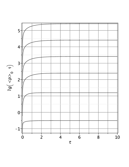
In particular, the integration of the relation (9) confirmed insensitivity of value from the number of parameters and, practically, confirmed the estimation formula (89) [1]
| (17) |
which did not account the details of the logarithmical dependency of the parameter on time. On Fig. 3 the results of this value’s numerical integration are shown.
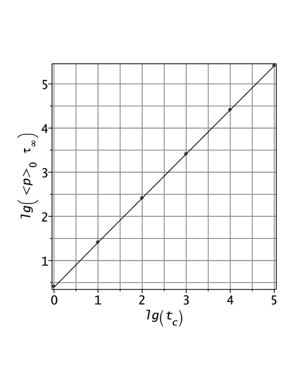
These results are well described by formula
| (18) |
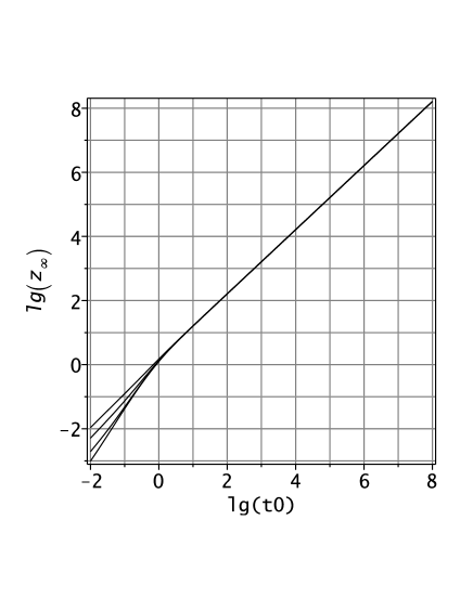
On Fig. 4 the dependency of the variable Z(t) at different values of time cosmological constant is shown.
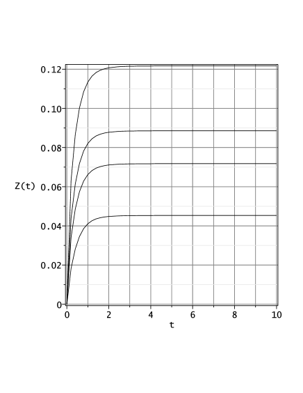
As it is follows from the results represented on this figure, function’s value also has a limit value at :
| (19) |
According to (47) [1]
| (20) |
this means that at superthermal particles’ distribution is “frozen”:
| (21) |
Thus, in modern Universe there can remain the “tail” of non-equilibrium particles of extra-high energies:
| (22) |
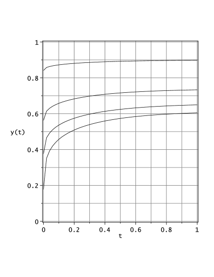
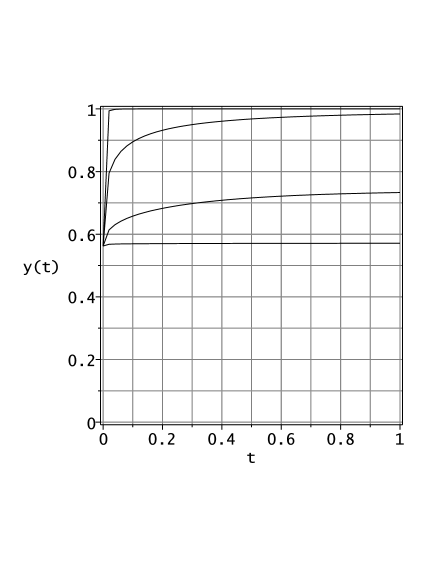
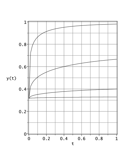
On Fig. 6–7 the results of numerical integration for the relative temperature are shown. According to the meaning of that value the dimensionless parameter:
| (23) |
is a relative part of cosmological plasma’s energy concluded in this non-equilibrium “tail” of distribution.
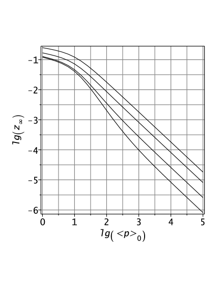
2.3 Asymptotic values of parametres of nonequilibrium distribution at an inflationary stage
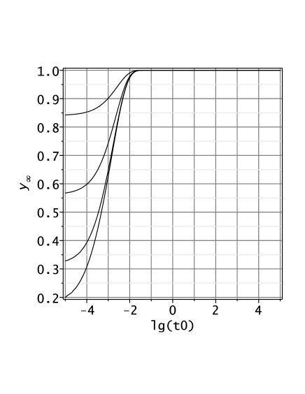
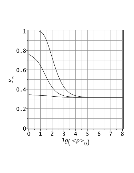
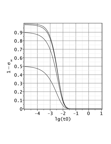
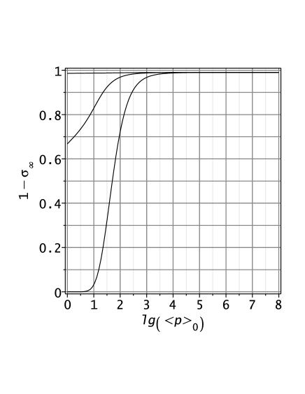
For supervision in present epoch the Universe the knowledge of possible limiting values of parametres of nonequilibrium distribution of particles is important. Such probable observable parametres are, first, relative temperature, , the relative part of energy concluded in a nonequilibrium tail of distribution, and also the form of this distribution. On Fig. 8, 9, 10, 11, 12, 13 the calculated values of the first two parametres are present.
2.4 Analysis of numerical simulation
From these results follows, that already at values of parameter an order 10-100 the survival of considerable number of nonequilibrium relic particles at a modern stage of evolution of the Universe is probable. It is the striking fact if to recollect, that according to results of early works of the Author in the standard cosmological scenario, deprived of an inflationary stage, at a modern stage only relic particles with energy of an order Gev and above can survive. At presence of a modern inflationary stage nonequilibrium relic particles with energy of an order 1 ev can survive!
On Fig. 14 the evolution of distribution of density of energy of nonequilibrium particles in the assumption of their initial distribution in form
| (24) |
is present.
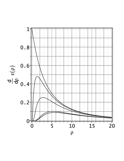
Calculating a maximum of distribution of density of energy from a relationship (20), we will find:
| (25) |
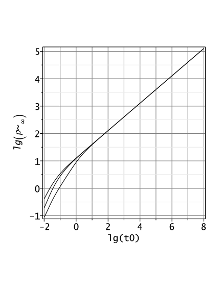
On Fig. 15 dependence of a maximum of a energy spectrum of nonequilibrium particles on cosmological constant is present. Apparently from this figure, at not so great values of a cosmological constant the maximum of a energy spectrum of nonequilibrium particles lays in the field of enough low energies, that, of course, does probable their detection in space conditions.
Conclusion
In the conclusion the Author once again expresses gratitude to professor Vitaly Melnikov for extremely fruitful question.
References
- [1] Yu.G. Ignat’ev. Russian Physics Journal, Vol. 56, No. 6, 2013, p. 745-751
- [2] Yurii Ignatyev, arXiv:1306.3633v1 [gr-qc] 13 June 2013; Yu.G. Ignatyev, Grav. and Cosmol., to be publish in vol. 19, No 4, 2013.
- [3] Yu.G. Ignat’ev, J. Sov. Phys. (Izv. Vuzov). 29, No 2, 19 (1986).
- [4] Yu.G.Ignatyev, D.Yu.Ignatyev, Gravitation & Cosmology Vol.13 (2007), No. 2 (50), pp. 101-113
- [5] Yu.G. Ignat’ev. Russian Physics Journal, to be publish in Vol. 56, No. 12, 2013.