Computation of summaries using net unfoldings

Abstract

We study the following summarization problem: given a parallel composition $\mathbf{A}=\mathcal{A}_{1}\parallel\ldots\parallel\mathcal{A}_{n}$ of labelled transition systems communicating with the environment through a distinguished component $\mathcal{A}_{i}$, efficiently compute a summary ${\cal S}_{i}$ such that $\mathbf{E}\parallel\mathbf{A}$ and $\mathbf{E}\parallel{\cal S}_{i}$ are trace-equivalent for every environment $\mathbf{E}$. While ${\cal S}_{i}$ can be computed using elementary automata theory, the resulting algorithm suffers from the state-explosion problem. We present a new, simple but subtle algorithm based on net unfoldings, a partial-order semantics, give some experimental results using an implementation on top of Mole, and show that our algorithm can handle divergences and compute weighted summaries with minor modifications.

1 Introduction

We address a fundamental problem in automatic compositional verification. Consider a parallel composition $\mathbf{A}=\mathcal{A}_{1}\parallel\ldots\parallel\mathcal{A}_{n}$ of processes, modelled as labelled transition systems, which is itself part of a larger system $\mathbf{E}\parallel\mathbf{A}$ for some environment $\mathbf{E}$. Assume that $\mathcal{A}_{i}$ is the interface of $\mathbf{A}$ with the environment, i.e., $\mathbf{A}$ communicates with the outer world only through actions of $\mathcal{A}_{i}$. The task consists in computing a new interface ${\cal S}_{i}$ with the same set of actions as $\mathcal{A}_{i}$ such that $\mathbf{E}\parallel\mathbf{A}$ and $\mathbf{E}\parallel{\cal S}_{i}$ have the same behaviour. In other words, the environment $E$ cannot distinguish between $\mathbf{A}$ and ${\cal S}_{i}$. Since ${\cal S}_{i}$ usually has a much smaller state space than $\mathbf{A}$ (making $\mathbf{E}\parallel\mathbf{A}$ easier to analyse) we call it a summary.

We study the problem in a CSP-like setting [13]: parallel composition is by rendez-vous, and the behaviour of a transition system is given by its trace semantics.

It is easy to compute ${\cal S}_{i}$ using elementary automata theory: we first compute the transition system of $\mathbf{A}$, whose states are tuples $(s_{1},\ldots,s_{n})$, where $s_{i}$ is a state of $\mathcal{A}_{i}$. Then we hide all actions except those of the interface, i.e., we replace them by $\varepsilon$-transitions ($\tau$-transitions in CSP terminology). We can then eliminate all $\varepsilon$-transitions using standard algorithms, and, if desired, compute the minimal summary by applying e.g. Hopcroft’s algorithm. The problem of this approach is the state-space explosion: the number of states of $\mathbf{A}$ can grow exponentially in the number of sequential components. While this is unavoidable in the worst case (deciding whether ${\cal S}_{i}$ has an empty set of traces is a PSPACE-complete problem, and the minimal summary ${\cal S}_{i}$ may be exponentially larger than $\mathcal{A}_{1},\ldots,\mathcal{A}_{n}$ in the worst case, see e.g. [11]) the combinatorial explosion happens already in trivial cases: if the components $\mathcal{A}_{1},\ldots,\mathcal{A}_{n}$ do not communicate at all, we can obviously take ${\cal S}_{i}=\mathcal{A}_{i}$, but the algorithm we have just described will need exponential time and space.

We present a technique to palliate this problem based on net unfoldings (see e.g. [4]). Net unfoldings are a partial-order semantics for concurrent systems, closely related to event structures [24], that provides very compact representations of the state space for systems with a high degree of concurrency. Intuitively, an unfolding is the extension to parallel compositions of the notion of unfolding a transition system into a tree. The unfolding is usually infinite. We show how to algorithmically construct a finite prefix of it from which the summary can be easily extracted. The algorithm can be easily implemented re-using many components of existing unfolders like Punf [14] and Mole [22]. However, its correctness proof is surprisingly subtle. This proof is the main contribution of the paper. However, we also evaluate the algorithm on some classical benchmarks [2]. We then show that – with minor modifications – the algorithm can be extended so that the summary obtained contains information about the possible divergences, that is whether or not after a given finite trace of the interface $\mathcal{A}_{i}$ it is possible that $\mathbf{A}$ evolves silently forever (i.e. without using any action of $\mathcal{A}_{i}$). And finally, we show how to extend the algorithm to deal with weighted systems: ${\cal S}_{i}$ then also gives for each of its finite traces the minimum cost in $\mathbf{A}$ to execute this trace.

Related work. The summarization problem has been extensively studied in an interleaving setting (see e.g. [10, 23, 25]), in which one first constructs the transition system of $\mathbf{A}$ and then reduces it. We study it in a partial-order setting.

Net unfoldings, and in general partial-order semantics, have been used to solve many analysis problems: deadlock [19, 16], reachability and model-checking questions [6, 3, 15, 4, 1], diagnosis [7], and other specific applications [18, 12]. To the best of our knowledge we are the first to explicitly study the summarization problem.

Our problem can be solved with the help of Zielonka’s algorithm [26, 20, 9], which yields an asynchronous automaton trace-equivalent to $\mathbf{A}$. The projection of this automaton onto the alphabet of $\mathcal{A}_{i}$ yields a summary ${\cal S}_{i}$. However, Zielonka’s algorithm is notoriously complicated and, contrary to our algorithm, requires to store much additional information for each event [20]. In [8], the complete tuple ${\cal S}_{1},\ldots,{\cal S}_{n}$ is computed – possibly in a weighted context – with an iterative message-passing algorithm that transfers information between components until a fixed point is reached. However, termination is only guaranteed when the communication graph is acyclic.

This paper extends [5] with proofs and implementation details.

2 Preliminaries

2.1 Transition systems

A labelled transition system (LTS) is a tuple $\mathcal{A}=(\Sigma,S,T,\lambda,s^{0})$ where $\Sigma$ is a set of actions, $S$ is a set of states, $T\subseteq S\times S$ is a set of transitions, $\lambda\colon T\rightarrow\Sigma$ is a labelling function, and $s^{0}\in S$ is an initial state. An $a$-transition is a transition labelled by $a$. We use this definition – excluding the possibility to have two transitions with different labels between the same pair of states – for simplicity. However, the results presented in this paper would still hold if this possibility was not excluded. A sequence of transitions $\tau=t_{1}t_{2}t_{3}\dots\in T^{*}\cup T^{\omega}$ is an execution of $\mathcal{A}$ if there is a sequence $s_{0}s_{1}s_{2}\dots$ of states such that $t_{k}=(s_{k-1},s_{k})$ for every $k$. We write $s_{0}\mathop{{\hbox{{$\buildrel\quad\scriptstyle{\tau}\quad\over{\hbox to10.06009pt{\rightarrowfill}}$}}}}$ (or $s_{0}\mathop{{\hbox{{$\buildrel\quad\scriptstyle{\tau}\quad\over{\hbox to10.06009pt{\rightarrowfill}}$}}}}s_{n}$ when $\tau$ is finite with $t_{n}$ as last transition). An execution is a history if $s_{0}=s^{0}$. A sequence $\sigma=a_{1}a_{2}a_{3}\ldots\in\Sigma^{*}\cup\Sigma^{\omega}$ of actions is a computation if there is an execution $\tau=t_{1}t_{2}t_{3}\dots$ such that $\lambda(\tau)=\lambda(t_{1})\lambda(t_{2})\lambda(t_{3})\ldots=\sigma$; if $s_{0}\mathop{{\hbox{{$\buildrel\quad\scriptstyle{\tau}\quad\over{\hbox to10.06009pt{\rightarrowfill}}$}}}}$, then we also write $s_{0}\mathop{{\hbox{{$\buildrel\quad\scriptstyle{\sigma}\quad\over{\hbox to10.99991pt{\rightarrowfill}}$}}}}$. It is a trace iff there exists such $\tau$ which is an history. We call $\tau$ a realization of $\sigma$. Abusing language, given an execution $\tau=t_{1}t_{2}t_{3}\ldots$, we denote by $tr(\tau)$ the computation $\lambda(t_{1})\lambda(t_{2})\lambda(t_{3})\ldots$ (even if it is not necessarily a trace). The set of traces of $\mathcal{A}$ is denoted by ${\it Tr}(\mathcal{A})$. Figure 1 shows (on its left) three transition systems.

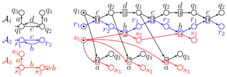
Figure 1: Three labeled transition systems (left) and a branching process (right)

Let $\mathcal{A}_{1},\dots,\mathcal{A}_{n}$ be LTSs where $\mathcal{A}_{i}=(\Sigma_{i},S_{i},T_{i},\lambda_{i},s^{0}_{i})$. The parallel composition $\mathbf{A}=\mathcal{A}_{1}\parallel\ldots\parallel\mathcal{A}_{n}$ is the LTS defined as follows. The set of actions is $\mathbf{\Sigma}=\Sigma_{1}\cup\ldots\cup\Sigma_{n}$. The states, called global states, are the tuples $\mathbf{s}=(s_{1},\dots,s_{n})$ such that $s_{i}\in S_{i}$ for every $i\in\{1..n\}$. The initial global state is $\mathbf{s}^{0}=(s_{1}^{0},\dots,s_{n}^{0})$. The transitions, called global transitions, are the tuples $\mathbf{t}=(t_{1},\ldots,t_{n})\in(T_{1}\cup\{\star\})\times\dots\times(T_{n}\cup\{\star\})\setminus\{(\star,\dots,\star)\}$ such that there is an action $a\in\mathbf{\Sigma}$ satisfying for every $i\in\{1..n\}$: if $a\in\Sigma_{i}$, then $t_{i}$ is an $a$-transition of $T_{i}$, otherwise $t_{i}=\star$; the label of $\mathbf{t}$ is the action $a$. If $t_{i}\neq\star$ we say that $\mathcal{A}_{i}$ participates in $\mathbf{t}$. It is easy to see that $\sigma\in\mathbf{\Sigma}^{*}\cup\mathbf{\Sigma}^{\omega}$ is a trace of $\mathbf{A}$ iff for every $i\in\{1..n\}$ the projection of $\sigma$ on $\Sigma_{i}$, denoted by $\sigma_{|\Sigma_{i}}$, is a trace of $\mathcal{A}_{i}$.

2.2 Petri nets

A labelled net is a tuple $(\Sigma,P,T,F,\lambda)$ where $\Sigma$ is a set of actions, $P$ and $T$ are disjoint sets of places and transitions (jointly called nodes), $F\subseteq(P\times T)\cup(T\times P)$ is a set of arcs, and $\lambda\colon P\cup T\rightarrow\Sigma$ is a labelling function. For $x\in P\cup T$ we denote by ${}^{\bullet}\!{x}=\{\,y\mid(y,x)\in F\,\}$ and ${x}^{\bullet}=\{\,y\mid(x,y)\in F\,\}$ the sets of inputs and outputs of $x$, respectively. A set $M$ of places is called a marking. A labelled Petri net is a tuple $\mathcal{N}=(\Sigma,P,T,F,\lambda,M_{0})$ where $(\Sigma,P,T,F,\lambda)$ is a labelled net and $M_{0}\subseteq P$ is the initial marking. A marking $M$ enables a transition $t\in T$ if ${}^{\bullet}\!{t}\subseteq M$. In this case $t$ can occur or fire, leading to the new marking $M^{\prime}=(M\setminus{}^{\bullet}\!{t})\cup{t}^{\bullet}$. An occurrence sequence is a (finite or infinite) sequence of transitions that can occur from $M_{0}$ in the order specified by the sequence. A trace is the sequence of labels of an occurrence sequence. The set of traces of $\mathcal{N}$ is denoted by ${\it Tr}(\mathcal{N})$.

2.3 Branching processes

The finite branching processes of $\mathbf{A}=\mathcal{A}_{1}~{}\parallel~{}\ldots~{}\parallel~{}\mathcal{A}_{n}$ are labelled Petri nets whose places are labelled with states of $\mathcal{A}_{1},\dots,\mathcal{A}_{n}$, and whose transitions are labelled with global transitions of $\mathbf{A}$. Following tradition, we call the places and transitions of these nets conditions and events, respectively. (Since global transitions are labelled with actions, each event is also implicitly labelled with an action.) We say that a marking $M$ of these nets enables a global transition $\mathbf{t}$ of $\mathbf{A}$ if for every state $s\in{}^{\bullet}\!{\mathbf{t}}$ some condition of $M$ is labelled by $s$. The set of finite branching processes of $\mathbf{A}$ is defined inductively as follows:

1. A labelled Petri net with conditions $b_{1}^{0},...,b_{n}^{0}$ labelled by $s_{1}^{0},\ldots,s_{n}^{0}$, no events, and with initial marking $\{b_{1}^{0},...,b_{n}^{0}\}$, is a branching process of $\mathbf{A}$.

2. Let $\mathcal{N}$ be a branching process of $\mathbf{A}$ such that some reachable marking of $\mathcal{N}$ enables some global transition $\mathbf{t}$. Let $M$ be the subset of conditions of the marking labelled by ${}^{\bullet}\!{\mathbf{t}}$. If $\mathcal{N}$ has no event labelled by $\mathbf{t}$ with $M$ as input set, then the Petri net obtained by adding to $\mathcal{N}$: a new event $e$, labelled by $\mathbf{t}$; a new condition for every state $s$ of ${\mathbf{t}}^{\bullet}$, labelled by $s$; new arcs leading from each condition of $M$ to $e$, and from $e$ to each of the new conditions, is also a branching process of $\mathbf{A}$.

Figure 1 shows on the right a branching process of the parallel composition of the LTSs on the left. Events are labelled with their corresponding actions.

The set of all branching processes of a net, finite and infinite, is defined by closing the finite branching processes under countable unions (after a suitable renaming of conditions and events) [4]. In particular, the union of all finite branching processes yields the unfolding of the net, which intuitively corresponds to the result of exhaustively adding all extensions in the definition above.

A trace of a branching process $\mathcal{N}$ is the sequence of action labels of an occurrence sequence of events of $\mathcal{N}$. In Figure 1, firing the events on the top half of the process yields any of the traces $cbdcbd$, $cdbcbd$, $cbdcdb$, or $cdbcdb$. The sets of traces of $\mathbf{A}$ and of its unfolding coincide.

Let $x,y$ be nodes of a branching process. We say that $x$ is a causal predecessor of $y$, denoted by $x<y$, if there is a non-empty path of arcs from $x$ to $y$; further, $x\leq y$ denotes that either $x<y$ or $x=y$. If $x\leq y$ or $x\geq y$, then $x$ and $y$ are causally related. We say that $x$ and $y$ are in conflict, denoted by $x\mathrel{\#}y$, if there is a condition $z$ (different from $x$ and $y$) from which one can reach both $x$ and $y$, exiting $z$ by different arcs. Finally, $x$ and $y$ are concurrent if they are neither causally related nor in conflict.

A set of events $E$ is a configuration if it is causally closed (that is, if $e\in E$ and $e^{\prime}<e$ then $e^{\prime}\in E$) and conflict-free (that is, for every $e,e^{\prime}\in E$, $e$ and $e^{\prime}$ are not in conflict). The past of an event $e$, denoted by $[e]$, is the set of events $e^{\prime}$ such that $e^{\prime}\leq e$ (so it is a configuration). For any event $e$, we denote by $M(e)$ the unique marking reached by any occurrence sequence that fires exactly the events of $[e]$. Notice that, for each component $\mathcal{A}_{i}$ of $\mathbf{A}$, $M(e)$ contains exactly one condition labelled by a state of $\mathcal{A}_{i}$. We denote this condition by $M(e)_{i}$. We write $\mathbf{St}(e)=\{\,\lambda(x)\mid x\in M(e)\,\}$ and call it the global state reached by $e$.

3 The Summary Problem

Let $\mathbf{A}=\mathcal{A}_{1}\parallel\dots\parallel\mathcal{A}_{n}$ be a parallel composition with a distinguished component $\mathcal{A}_{i}$, called the interface. An environment of $\mathbf{A}$ is any LTS $\mathbf{E}$ (possibly a parallel composition) that only communicates with $\mathbf{A}$ through the interface, i.e, $\Sigma_{\mathbf{E}}\cap(\Sigma_{1}\cup\ldots\cup\Sigma_{n})=\Sigma_{\mathbf{E}}\cap\Sigma_{i}$. We wish to compute a summary ${\cal S}_{i}$, i.e., an LTS with the same actions as $\mathcal{A}_{i}$ such that ${\it Tr}(\mathbf{E}\parallel\mathbf{A})|_{\Sigma_{\mathbf{E}}}={\it Tr}(\mathbf{E}\parallel{\cal S}_{i})|_{\Sigma_{\mathbf{E}}}$ for every environment $\mathbf{E}$, where $X|_{\Sigma}$ denotes the projection of the traces of $X$ onto $\Sigma$. It is well known (and follows easily from the definitions) that this holds iff ${\it Tr}({\cal S}_{i})={\it Tr}(\mathbf{A})|_{\Sigma_{i}}$ [13]. We therefore address the following problem:

Definition 1 (Summary problem)

Given LTSs $\mathcal{A}_{1},\ldots,\mathcal{A}_{n}$ with interface $\mathcal{A}_{i}$, compute an LTS ${\cal S}_{i}$ satisfying ${\it Tr}({\cal S}_{i})={\it Tr}(\mathbf{A})|_{\Sigma_{i}}$, where $\mathbf{A}=\mathcal{A}_{1}\parallel\cdots\parallel\mathcal{A}_{n}$.

The problem can be solved by computing the LTS $\mathbf{A}$, but the size of $\mathbf{A}$ can be exponential in $\mathcal{A}_{1},\ldots,\mathcal{A}_{n}$. So we investigate an unfolding approach.

The interface projection $\mathcal{N}_{i}$ of a branching process $\mathcal{N}$ of $\mathbf{A}$ onto $\mathcal{A}_{i}$ is the following labelled subnet of $\mathcal{N}$: (1) the conditions of $\mathcal{N}_{i}$ are the conditions of $\mathcal{N}$ with labels in $S_{i}$; (2) the events of $\mathcal{N}_{i}$ are the events of $\mathcal{N}$ where $\mathcal{A}_{i}$ participates; (3) $(x,y)$ is an arc of $\mathcal{N}_{i}$ iff it is an arc of $\mathcal{N}$ and $(x,y)$ are nodes of $\mathcal{N}_{i}$. Obviously, every event of $\mathcal{N}_{i}$ has exactly one input and one output condition, and $\mathcal{N}_{i}$ can therefore be seen as an LTS; thus, we sometimes speak of the LTS $\mathcal{N}_{i}$. The interface projection $\mathcal{N}_{1}$ for the branching process of Figure 1 is the subnet given by the black conditions and their input and output events, and its LTS representation is shown in the left of Figure 2.

Figure 2: Projection of the branching process of Figure 1 on $\mathcal{A}_{1}$ (left) and a folding (right)

The projection $\mathcal{U}_{i}$ of the full unfolding of $\mathbf{A}$ onto $\mathcal{A}_{i}$ clearly satisfies ${\it Tr}(\mathcal{U}_{i})={\it Tr}(\mathbf{A})_{|\Sigma_{i}}$; however, $\mathcal{U}_{i}$ can be infinite. In the rest of the paper we show how to compute a finite branching process $\mathcal{N}$ and an equivalence relation $\equiv$ between the conditions of $\mathcal{N}_{i}$ such that the result of folding $\mathcal{N}_{i}$ into a finite LTS by merging the conditions of each equivalence class yields the desired ${\cal S}_{i}$. The folding of $\mathcal{N}_{i}$ is the LTS whose states are the equivalence classes of $\equiv$, and every transition $(s,s^{\prime})$ of $\mathcal{N}_{i}$ yields a transition $([s]_{\equiv},[s^{\prime}]_{\equiv})$ of the folding. Figure 2 shows on the right the result of folding the LTS on the left when the only equivalence class with more than one member is formed by the two rightmost states labelled by $q_{2}$.

We construct $\mathcal{N}$ by starting with the branching processes without events and iteratively add one event at a time. Some events are marked as cut-offs [4]. An event $e$ added to $\mathcal{N}$ becomes a cut-off if $\mathcal{N}$ already contains an $e^{\prime}$, called the companion of $e$, satisfying a certain, yet to be specified cut-off criterion. Events with cut-offs in their past cannot be added. The algorithm terminates when no more events can be added. The equivalence relation $\equiv$ is determined by the interface cut-offs: the cut-offs labelled with interface actions. If an interface cut-off $e$ has companion $e^{\prime}$, then we set $M(e)_{i}\equiv M(e^{\prime})_{i}$. Algorithm 1 is pseudocode for the unfolding, where $Ext(\mathcal{N},co)$ denotes the possible extensions: the events which can be added to $\mathcal{N}$ without events from the set $co$ of cut-offs in their past.

let $\mathcal{N}$ be the unique branching process of $\mathbf{A}$ without events and let $co=\emptyset$

While $Ext(\mathcal{N},co)\neq\emptyset$ do

     choose $e$ in $Ext(\mathcal{N},co)$ and extend $\mathcal{N}$ with $e$

     If $e$ is a cut-off event then let $co=co\cup\{e\}$

For every $e\in co$ with companion $e^{\prime}$ do merge $[M(e)_{i}]_{\equiv}$ and $[M(e^{\prime})_{i}]_{\equiv}$

Algorithm 1 Unfolding procedure for a product $\mathbf{A}$.

Notice that the algorithm is nondeterministic: the order in which events are added is not fixed (though it necessarily respects causal relations). We wish to find a definition of cut-offs such that the LTS ${\cal S}_{i}$ delivered by the algorithm is a correct solution to the summary problem. Several papers have addressed the problem of defining cut-offs such that the branching process delivered by the algorithm contains all global states of the system (see [4] and the references therein). We first remark that these approaches do not “unfold enough”.

Standard cut-off condition does not work.

Usually, an event $e$ is declared a cut-off if the branching process already contains an event $e^{\prime}$ with the same global state. If events are added according to an adequate order [4], then the prefix generated by the algorithm is guaranteed to contain occurrence sequences leading to all reachable markings.

We show that with this definition of cut-off even we do not always compute a correct summary. We do so by showing an example in which independently of the order in which Algorithm 1 adds events the summary is always wrong. Consider the parallel composition of Figure 3 with $\mathcal{A}_{1}$ as interface.

Figure 3: Three labeled transition systems (left) and a branching process (right)

Independently of the order in which events are added, the branching process $\mathcal{N}$ computed by Algorithm 1 is the one shown on the right of Figure 3. The only cut-off event is $5$, with companion event $2$, for which we have $\mathbf{St}(5)=\{q_{2},r_{1},s_{2}\}=\mathbf{St}(2)$. The interface projection $\mathcal{N}_{1}$ is the transition system in Figure 4.

Figure 4: Projection of the branching process of Figure 3 on $\mathcal{A}_{1}$

Since $\mathcal{N}_{1}$ does not contain any cut-off, its folding is again $\mathcal{N}_{1}$, and since ${\it Tr}(\mathbf{A})|_{\Sigma_{1}}\supseteq cdc(dc)^{*}$, $\mathcal{N}_{1}$ is not a summary.

4 Two Attempts

The solution turns out to be remarkably subtle, and so we approach it in a series of steps.

4.1 First attempt

In the following we shall call events in which $\mathcal{A}_{i}$ participates $i$-events for short; analogously, we call $i$-conditions the conditions labelled by states of $\mathcal{A}_{i}$.

The simplest idea is to declare an $i$-event $e$ a cut-off if the branching process already contains another $i$-event $e^{\prime}$ with $\mathbf{St}(e)=\mathbf{St}(e^{\prime})$. Intuitively, the behaviours of the interface after the configurations $[e]$ and $[e^{\prime}]$ is identical, and so we only explore the future of $[e^{\prime}]$.

Cut-off definition 1. An event $e$ is a cut-off event if it is an $i$-event and $\mathcal{N}$ contains an $i$-event $e^{\prime}$ such that $\mathbf{St}(e)=\mathbf{St}(e^{\prime})$.

It is not difficult to show that this definition is correct for non-divergent systems.

Definition 2

A parallel composition $\mathbf{A}$ with interface $\mathcal{A}_{i}$ is divergent if some infinite trace of $\mathbf{A}$ contains only finitely many occurrences of actions of $\Sigma_{i}$.

Theorem 4.1

Let $\mathbf{A}$ be non-divergent. The instance of Algorithm 1 with cut-off definition 1 terminates with a finite branching process $\mathcal{N}$, and the folding ${\cal S}_{i}$ of $\mathcal{N}_{i}$ is a summary of $\mathbf{A}$.

Proof

Let $\mathcal{N}$ be the branching process constructed by Algorithm 1. Assume $\mathcal{N}$ is infinite (i.e., the algorithm does not terminate). Then $\mathcal{N}$ contains an infinite chain $e_{1}<e_{2}\cdots$ of causally related events [17]. Since $\mathbf{A}$ is non-divergent, the infinite configuration $C=\bigcup_{i=1}^{\infty}[e_{i}]$ contains infinitely many $i$-events. Since the interface $\mathcal{A}_{i}$ participates in all of them, they are all causally related, and so $C$ contains an infinite chain $e_{1}^{\prime}<e_{2}^{\prime}\ldots$ of causally related $i$-events. Since $\mathbf{A}$ has only finitely many global states, the chain contains two $i$-events $e_{j}^{\prime}<e_{k}^{\prime}$ such that $\mathbf{St}(e_{j}^{\prime})=\mathbf{St}(e_{k}^{\prime})$. So $e_{k}^{\prime}$ is a cut-off, in contradiction with the fact that $e_{k+1}^{\prime}$ belongs to $\mathcal{N}$. So $\mathcal{N}$ is finite, and so Algorithm 1 terminates.

It remains to prove ${\it Tr}({\cal S}_{i})={\it Tr}(\mathbf{A})|_{\Sigma_{i}}$. We prove both inclusions separately, but we first need some preliminaries. We extend the mapping $\mathbf{St}()$ to conditions by defining $\mathbf{St}(b)=\mathbf{St}(e)$, where $e$ is the unique input event of condition $b$. Since the states of ${\cal S}_{i}$ are equivalence classes of conditions of $\mathcal{N}_{i}$ and, by definition, if $b\equiv b^{\prime}$ then $\mathbf{St}(b)=\mathbf{St}(b^{\prime})$, we can extend $\mathbf{St}()$ further to equivalence classes by defining $\mathbf{St}([b]_{\equiv})=\mathbf{St}(b)$.

${\it Tr}({\cal S}_{i})\subseteq{\it Tr}(\mathbf{A})|_{\Sigma_{i}}$. Let $tr^{i}$ be a trace of ${\cal S}_{i}$. Then $[b^{0}]_{\equiv}\mathop{{\hbox{{$\buildrel\quad\scriptstyle{tr^{i}}\quad\over{\hbox to14.2584pt{\rightarrowfill}}$}}}}$ in ${\cal S}_{i}$, where $[b^{0}]_{\equiv}$ is the initial state of ${\cal S}_{i}$. By the definition of folding, there exist $tr^{i}_{1},tr^{i}_{2},tr^{i}_{3},\ldots$ (finite sequences of actions) and pairs $(b_{1}^{\prime},b_{1}),(b_{2}^{\prime},b_{2}),(b_{2}^{\prime},b_{2}),\ldots$ of conditions of $\mathcal{N}_{i}$ such that (1) $tr^{i}=tr^{i}_{1}tr^{i}_{2}tr^{i}_{3}\ldots$; (2) $b^{0}=b^{\prime}_{1}$; (3) $b_{j}^{\prime}\mathop{{\hbox{{$\buildrel\quad\scriptstyle{tr_{j}^{i}}\quad\over{\hbox to14.75655pt{\rightarrowfill}}$}}}}b_{j}$ in $\mathcal{N}_{i}$ for every $j$; and (4) $b_{j-1}\equiv b_{j}^{\prime}$ for every $j$.

By (3) and the definition of projection, we have $\mathbf{St}(b_{j}^{\prime})\mathop{{\hbox{{$\buildrel\quad\scriptstyle{tr_{j}}\quad\over{\hbox to14.75655pt{\rightarrowfill}}$}}}}\mathbf{St}(b_{j})$ in $\mathbf{A}$ for some $tr_{j}\in\Sigma^{*}$ such that $tr^{i}_{j}=tr_{j}|_{\Sigma_{i}}$: indeed, if $e$ and $e^{\prime}$ are the input events of $b_{j}$ and $b^{\prime}_{j}$, then $\mathbf{St}(b_{j})$ is reachable from $\mathbf{St}(b^{\prime}_{j-1})$ by means of any computation $tr_{j}$ corresponding to executing the events of $[e]\setminus[e^{\prime}]$, and any such $tr_{j}$ satisfies $tr^{i}_{j}=tr_{j}|_{\Sigma_{i}}$. Moreover, by (4) we have $\mathbf{St}(b_{j-1})=\mathbf{St}(b_{j}^{\prime})$. So we get

$$\mathbf{St}(b_{1}^{\prime})\mathop{{\hbox{{$\buildrel\quad\scriptstyle{tr_{1}}\quad\over{\hbox to14.88036pt{\rightarrowfill}}$}}}}\mathbf{St}(b_{2}^{\prime})\mathop{{\hbox{{$\buildrel\quad\scriptstyle{tr_{2}}\quad\over{\hbox to14.88036pt{\rightarrowfill}}$}}}}\mathbf{St}(b_{3}^{\prime})\mathop{{\hbox{{$\buildrel\quad\scriptstyle{tr_{3}}\quad\over{\hbox to14.88036pt{\rightarrowfill}}$}}}}\cdots$$

By (1) and (2) we have $\mathbf{St}(b^{0})\mathop{{\hbox{{$\buildrel\quad\scriptstyle{tr_{1}tr_{2}tr_{3}\dots}\quad\over{\hbox to35.89104pt{\rightarrowfill}}$}}}}$ in $\mathbf{A}$, and so $tr^{i}=tr|_{\Sigma_{i}}\in{\it Tr}(\mathbf{A})|_{\Sigma_{i}}$ with $tr=tr_{1}tr_{2}tr_{3}\dots$.

${\it Tr}(\mathbf{A})|_{\Sigma_{i}}\subseteq{\it Tr}({\cal S}_{i})$. Let $tr$ be a finite or infinite trace of $\mathbf{A}$. We prove that there exists a trace $tr^{i}$ of ${\cal S}_{i}$ such that $tr^{i}=tr|_{\Sigma_{i}}$. For that we prove that for every history $h$ of $\mathbf{A}$ there exists a history $h^{i}$ of ${\cal S}_{i}$ such that $tr(h^{i})=tr(h)|_{\Sigma_{i}}$.

A finite history $h=\mathbf{t}_{1}\ldots\mathbf{t}_{k}$ is short if the unique sequence of events of the unfolding $e_{1}\ldots e_{k}$ such that $\lambda(e_{\ell})=\mathbf{t}_{\ell}$ for every $\ell\in\{1..k\}$ satisfies the following conditions: $e_{\ell}\leq e_{k}$ for every $\ell\in\{1..k\}$, and $e_{k}$ is an $i$-event. (The name is due to the fact that, loosely speaking, $h$ is a shortest history in which $e_{k}$ occurs.)

We say that a finite or infinite history $h$ is succinct if there are $h_{1},h_{2},h_{3}\ldots$ such that $h=h_{1}h_{2}h_{3}\ldots$, $|tr(h_{k})|_{\Sigma_{i}}|=1$ for every $k$, and $h_{1}\ldots h_{\ell}$ is short for every $\ell$. We call $h_{1}h_{2}h_{3}\dots$ the $i$-decomposition of $h$. It is easy to see that for every history $h$ of $\mathbf{A}$ there exists a succinct history $h^{\prime}$ of $\mathbf{A}$ with the same projection onto $\mathcal{A}_{i}$ (let $o=o_{1}o_{2}o_{3}\dots$ be the occurrence sequence such that $\lambda(o)=h$, denote by $e_{i_{1}}e_{i_{2}}e_{i_{3}}\dots$ its $i$-events in the order they appear in $o$, then simply take for $h^{\prime}$ any history with $i$-decomposition $h^{\prime}_{1}h^{\prime}_{2}h^{\prime}_{3}\dots$ such that, for any $\ell$, $h^{\prime}_{1}\dots h^{\prime}_{\ell}$ is an history corresponding to $[e_{i_{\ell}}]$). So it suffices to prove the result for succinct histories.

We prove by induction the following stronger result. For every succinct history of $\mathbf{A}$ with $i$-decomposition $h_{1}h_{2}h_{3}\ldots$ there exist $h_{1}^{i},h_{2}^{i},h_{3}^{i},\dots$ such that for every $k$:

1. $H^{i}_{k}=h^{i}_{1}\dots h^{i}_{k}$ is an history of ${\cal S}_{i}$ such that $tr(H^{i}_{k})=tr(h_{1}\dots h_{k})|_{\Sigma_{i}}$.

2. There exists a configuration $C_{k}$ of $\mathcal{N}$ that contains no cut-offs and such that $[M(C_{k})_{i}]_{\equiv}$ is the state reached by $H^{i}_{k}$.

Base case. If $k=0$, then $H^{i}_{k}$ is the empty history of ${\cal S}_{i}$, take $C_{k}=\emptyset$.

Inductive step. Let $H_{k+1}$ be the prefix of $h$ with $i$-decomposition $H_{k+1}=h_{1}\ldots h_{k}h_{k+1}$ (it is a succinct history of $\mathbf{A}$). Then $H_{k}=h_{1}\ldots h_{k}$ is succinct with $i$-decomposition $h_{1}\ldots h_{k}$. By induction hypothesis $H_{k}^{i}=h_{1}^{i}\dots h_{k}^{i}$ and some configuration $C_{k}$ satisfy the conditions above.

Let $o_{k+1}=e_{1}\dots e_{m}$, where $m=|h_{k+1}|$, be the only sequence of events whose labelling is $h_{k+1}$ and can occur in the order of the sequence from the marking $M(C_{k})$ (this sequence always exists by the properties of $C_{k}$). Two cases are possible.

1. $o_{k+1}$ contains no cut-off. In this case $o_{k+1}$ is a sequence of events from $\mathcal{N}$ (because $C_{k}$ contains no cut-offs). Thus, there exists an execution $h_{i,k+1}$ of ${\cal S}_{i}$ from the state $[M(C_{k})_{i}]_{\equiv}$ to the state $[M(e_{m})_{i}]_{\equiv}$ such that $tr(h_{i,k+1})=tr(h_{k+1})|_{\Sigma_{i}}$. So we can take $h^{i}_{k+1}=h_{i,k+1}$. It remains to choose the configuration $C_{k+1}$. We take $C_{k+1}$ as $C_{k}\cup\{e_{1},\ldots,e_{m}\}$, which contains no cut-offs because $C_{k}$ contains no cut-offs by hypothesis.

2. $o_{k+1}$ contains some cut-off. Since $h_{k}$ is succinct, $e_{m}$ is the only $i$-event of $h_{k+1}$, and the only maximal event of $\{e_{1},\ldots,e_{m}\}$ w.r.t. the causal relation. Since only $i$-events can be cut-offs, $e_{m}$ is a cut-off, and the only cut-off among the events of $o_{k+1}$. So $o_{k+1}$ is a sequence of events from $\mathcal{N}$ whose last event is a cut-off. Further, by the maximality of $e_{m}$, the marking reached by $o_{k+1}$ is $M(e_{m})$. By the definition of folding, ${\cal S}_{i}$ has an execution $h_{i,k+1}$ from the state $[M(C_{k})_{i}]_{\equiv}$ to the state $[M(e_{m})_{i}]_{\equiv}$ such that $tr(h_{i,k+1})=tr(h_{k+1})|_{\Sigma_{i}}$. As above, this allows to take $h^{i}_{k+1}=h_{i,k+1}$.

   It remains to choose the configuration $C_{k+1}$. We cannot take $C_{k+1}=C_{k}\cup\{e_{1},\ldots,e_{m}\}$, because then $C_{k+1}$ would contain cut-offs. So we proceed differently. We choose $C_{k+1}=[e_{m}^{\prime}]$, where $e_{m}^{\prime}$ is the companion of $e_{m}$. Since $e_{m}^{\prime}$ is not a cut-off, $C_{k+1}$ contains no cut-offs. Moreover, since the marking reached by $o_{k+1}$ is $M(e_{m})$, we have that $[M(C_{k+1})_{i}]_{\equiv}$ is the state reached by $H_{k+1}^{i}$.

The system of Figure 1 is non-divergent. Algorithm 1 computes the branching process on the right of Figure 1. The only cut-off is event $9$ with companion $3$. The folding is shown in Figure 2 (right) and is a correct summary. However, cut-off definition 1 never works if $\mathbf{A}$ is divergent because the unfolding procedure does not terminate. Indeed, if the system has divergent traces then we can easily construct an infinite firing sequence of the unfolding such that none of the finitely many $i$-events in the sequence is a cut-off. Since no other events can be cut-offs, Algorithm 1 adds all events of the sequence. This occurs for instance for the system of Figure 5 with interface $\mathcal{A}_{1}$, where the occurrence sequence of the unfolding for the trace $\mathit{i}(\mathit{fcd})^{\omega}$ contains no cut-off.

4.2 Second attempt

To ensure termination for divergent systems, we extend the definition of cut-off. For this, we define for each event $e$ its $i$-predecessor. Intuitively, the $i$-predecessor of an event $e$ is the last condition that $e$ “knows” has been reached by the interface.

Definition 3

The $i$-predecessor of an event $e$, denoted by $ip(e)$, is the condition $M(e)_{i}$.

Assume now that two events $e_{1}<e_{2}$, neither of them interface event, satisfy $ip(e_{1})=ip(e_{2})$ and $\mathbf{St}(e_{1})=\mathbf{St}(e_{2})$. Then any occurrence sequence $\sigma$ that executes the events of the set $[e_{2}]\setminus[e_{1}]$ leads from a marking to itself and contains no interface events. So $\sigma$ can be repeated infinitely often, leading to an infinite trace with only finitely many interface actions. It is therefore plausible to mark $e_{2}$ as cut-off event, in order to avoid this infinite repetition.

Cut-off definition 2. An event $e$ is a cut-off if

1. $e$ is an $i$-event, and $\mathcal{N}$ contains an $i$-event $e^{\prime}$ with $\mathbf{St}(e)=\mathbf{St}(e^{\prime})$, or

2. $e$ is not an $i$-event, and some event $e^{\prime}<e$ satisfies $\mathbf{St}(e)=\mathbf{St}(e^{\prime})$ and $ip(e)=ip(e^{\prime})$.

We give an example showing that this natural definition does not work: the algorithm always terminates but can yield a wrong result. Consider the parallel composition at the left of Figure 5, with interface $\mathcal{A}_{1}$. Clearly ${\it Tr}(\mathcal{A})|_{\Sigma_{1}}={\it Tr}(A_{1})=iab^{*}e$. For any strategy the algorithm generates the branching process $\mathcal{N}$ at the top right of the figure (without the dashed part). $\mathcal{N}$ has two cut-off events: the interface event $6$, which is of type (1), and event $8$, a non-interface event, of type (2). Event $6$ has $5$ as companion, with $\mathbf{St}(5)=\mathbf{St}(6)=\{q_{2},r_{2},s_{2}\}$. Event $8$ has $0$ as companion, with $\mathbf{St}(0)=\{q_{1},r_{1},s_{1}\}=\mathbf{St}(8)$; moreover, $0<8$ and $ip(0)=ip(8)$. The folding of $\mathcal{N}_{1}$ is shown at the bottom right of the figure. It is clearly not trace-equivalent to $\mathcal{A}_{1}$ because it “misses” the trace $iabe$. The dashed event at the bottom right, which would correct this, is not added by the algorithm because it is a successor of $8$.

Figure 5: Cut-off definition 2 produces an incorrect result on $\mathbf{A}=\mathcal{A}_{1}\parallel\mathcal{A}_{2}\parallel\mathcal{A}_{3}$

5 The Solution

Intuitively, the reason for the failure of our second attempt on the example of Figure 5 is that $\mathcal{A}_{1}$ can only execute $iabe$ if $\mathcal{A}_{2}$ and $\mathcal{A}_{3}$ execute $\mathit{ifcd}$ first. However, when the algorithm observes that the markings before and after the execution of $\mathit{ifcd}$ are identical, it declares $8$ a cut-off event, and so it cannot “use” it to construct event $e$. So, on the one hand, $8$ should not be a cut-off event. But, on the other hand, some event of the trace $\mathit{i}(\mathit{fcd})^{\omega}$ must be declared cut-off, otherwise the algorithm does not terminate.

The way out of this dilemma is to introduce cut-off candidates. If an event is declared a cut-off candidate, the algorithm does not add any of its successors, just as with regular cut-offs. However, cut-off candidates may stop being candidates if the addition of a new event frees them. (So, an event is a cut-off candidate with respect to the current branching process.) A generic unfolding procedure using these ideas is given in Algorithm 2, where $Ext(\mathcal{N},co,coc)$ denotes the possible extensions of $\mathcal{N}$ that do not have any event of $co$ or $coc$ in their past. Assuming suitable definitions of cut-off candidates and freeing, the algorithm would, in our example, declare event $8$ a cut-off candidate, momentarily stop adding any of its successors, but later free event $8$ when event $5$ is discovered.

let $\mathcal{N}$ be the unique branching process of $\mathbf{A}$ without events; let $co=\emptyset$ and $coc=\emptyset$

While $Ext(\mathcal{N},co,coc)\neq\emptyset$ do

     choose $e$ in $Ext(\mathcal{N},co,coc)$ according to the search strategy

     If $e$ is a cut-off event then let $co=co\cup\{e\}$

     Elseif $e$ is a cut-off candidate of $\mathcal{N}$ then let $coc=coc\cup\{e\}$

     Else for every $e^{\prime}\in coc$ do

        If $e$ frees $e^{\prime}$ then $coc=coc\setminus\{e^{\prime}\}$

     extend $\mathcal{N}$ with $e$

For every $e\in co$ with companion $e^{\prime}$ do merge $[M(e)_{i}]_{\equiv}$ and $[M(e^{\prime})_{i}]_{\equiv}$

Algorithm 2 Unfolding procedure for a product $\mathbf{A}$.

The main contribution of our paper is the definition of a correct notion of cut-off candidate for the projection problem. We shall declare event $e$ a cut-off candidate if $e$ is not an interface event, and $\mathcal{N}$ contains a companion $e^{\prime}<e$ such that $\mathbf{St}(e^{\prime})=\mathbf{St}(e)$, $ip(e)=ip(e^{\prime})$, and, additionally, no interface event $e^{\prime\prime}$ of $\mathcal{N}$ is concurrent with $e$ without being concurrent with $e^{\prime}$. As long as this condition holds, the successors of $e$ are put “on hold”. In the example of Figure 5, if the algorithm first adds events $0$, $3$, $4$, and $8$, then event $8$ becomes a cut-off candidate with $0$ as companion. However, the addition of the interface event $5$ frees event $8$, because $5$ is concurrent with $8$ and not with $0$.

However, we are not completely done yet. The parallel composition at the left of Figure 6 gives an example in which even with this notion of cut-off candidate the result is still wrong. $\mathcal{A}_{1}$ is the interface. One branching process is represented at the top right of the figure. Event 3 (concurrent with 1) is a cut-off candidate with 2 (concurrent with 1, 4, and 5) as companion. This prevents the lower dashed part of the net to be added. Event 6 is cut-off with 1 as companion. This prevents the upper dashed part of the net to be added. The refolding obtained then (bottom right) does not contain the word $abcb$.

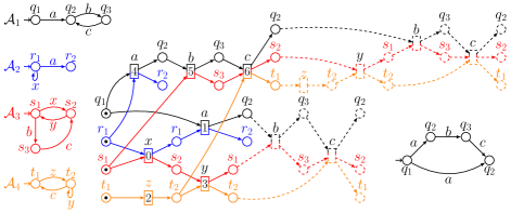
Figure 6: An example illustrating the use of strong causality

If we wish a correct algorithm for all strategies, we need a final touch: replace the condition $e^{\prime}<e$ by $e^{\prime}\ll e$, where $\ll$ is the strong causal relation:

Definition 4

Event $e^{\prime}$ is a strong cause of event $e$, denoted by $e^{\prime}\ll e$, if $e^{\prime}<e$ and $b^{\prime}<b$ for every $b\in M(e)\setminus M(e^{\prime}),b^{\prime}\in M(e^{\prime})\setminus M(e)$.

Using this definition, event 3 is no longer a cut-off candidate in the branching process of Figure 6 as it is not in strong causal relation with its companion 2 (because the $t_{2}$-labelled condition just after 2 belongs to $M(2)\setminus M(3)$ and is not causally related with the $r_{1}$-labelled condition just after $0$ which belongs to $M(3)\setminus M(2)$).

The two following lemma give properties of the strong causal relation that will be useful to prove our main result (Theorem 5.1).

Lemma 1

Every infinite chain $e_{1}<e_{2}<e_{3}\cdots$ of events of a branching process contains a strong causal subchain $e_{i_{1}}\ll e_{i_{2}}\ll e_{i_{3}}\cdots$.

Proof

Let $E=\{e_{1},e_{2},\dots\}$. Say that a component $\mathcal{A}_{j}$ of $\mathbf{A}$ participates in an event $e$ if it participates in the transition labelling $e$. We partition the (indices of the) components into the set $S$ of indices $j$ such that $\mathcal{A}_{j}$ participates in finitely many events of $E$, and $\bar{S}=\{1,\ldots,n\}\setminus S$. We say that the LTS $\mathcal{A}_{j}$ has stabilized at event $e_{k}$ in the chain if $\mathcal{A}_{j}$ does not participate in any event $e\geq e_{k}$. Let $e_{\alpha}$ be any event of $E$ such that all LTSs of $S$ have stabilized before $e_{\alpha}$. We claim that there exists $e_{\gamma}$ in $E$ such that $e_{\alpha}\ll e_{\gamma}$. Since clearly all LTSs of $S$ have also stabilized before $e_{\gamma}$, A repeated application of the claim produces the desired subsequence. The claim itself is proved in two steps:

• There exists $e_{\beta}>e_{\alpha}$ in $E$ such that $M(e_{\beta})_{k}\neq M(e_{\alpha})_{k}$ for every $k\in\bar{S}$, (which implies $M(e_{\alpha})_{k}<e_{\beta}$ for every $k\in\bar{S}$).
  The existence of $e_{\beta}$ follows from (1) the fact that all events of $E$ are causally related, and (2) the definition of $\bar{S}$, which implies for any $k\in\bar{S}$ the existence of an infinite subchain $e_{\ell_{1}}<e_{\ell_{2}}<\dots$ such that $M(e_{\ell_{i}})_{k}\neq M(e_{\ell_{j}})_{k}$ for every $i,j$.

• There exists $e_{\gamma}>e_{\beta}$ in $E$ such that $M(e_{\gamma})_{k}>e_{\beta}$ for every $k\in\bar{S}$.
  Observe that if $e<M(e_{i})_{k}$ for some $i$ and some $k$, then $e<M(e_{j})_{k}$ for all $j>i$ (as $\forall i,j,\forall k,M(e_{i})_{k}\leq M(e_{j})_{k}$). Suppose that $e_{\gamma}$ does not exist. Then there exists $k\in\bar{S}$ such that $M(e^{\prime})_{k}\ngtr e$ for every $e^{\prime}>e$. As $k\in\bar{S}$, there exists, by definition, an infinite subchain $e<e_{\ell_{1}}<e_{\ell_{2}}\dots$ of $E$ such that $M(e_{\ell_{i}})_{k}\neq M(e_{\ell_{j}})_{k}$ for every $i,j$. So for any of these $e_{\ell_{i}}$ there exists a $k$-event $e_{\ell_{i}}^{\prime}$ such that $e_{\ell_{i}}^{\prime}<e_{\ell_{i}}$ and $e_{\ell_{i}}^{\prime}$ is concurrent with $e_{\ell_{i-1}}$. Let $e_{\ell_{i}}^{\prime\prime}$ be an event on a path from $e_{\ell_{i}}^{\prime}$ to $e_{\ell_{i}}$ and such that $b>e$ and $b^{\prime}\ngtr e$ for some $b,b^{\prime}\in{}^{\bullet}\!{e_{\ell_{i}}^{\prime\prime}}$ (the existence of such an event is ensured by the fact that $M(e_{\ell_{i}})_{k}\ngtr e$). As $b>e$ we get $e_{\ell_{i}}^{\prime\prime}>e$ and thus $b^{\prime\prime}>e$ for every $b^{\prime\prime}\in{e_{\ell_{i}}^{\prime\prime}}^{\bullet}$. Hence, by the observation above, the set $\{k\in\bar{S}~{}:~{}M(e_{\ell_{i}})_{k}>e\}$ is strictly greater than the set $\{k\in\bar{S}~{}:~{}M(e_{\ell_{i-1}})_{k}>e\}$. Since $\mathbf{A}$ is finite, this contradicts the existence of $k\in\bar{S}$ such that $M(e^{\prime})_{k}\ngtr e$ for every $e^{\prime}>e$ in $E$. So the event $e_{\gamma}$ exists.

It follows immediately from (1) and (2) that $e_{\alpha}\ll e_{\gamma}$ (because for any $k,k^{\prime}$, $M(e_{\alpha})_{k}<e_{\beta}<M(e_{\gamma})_{k^{\prime}}$), and all LTSs of $S$ have stabilized before $e_{\gamma}$, and so the claim is proved.

Lemma 2

If $e^{\prime}\ll e$ and $\hat{e}$ is concurrent with both $e^{\prime}$ and $e$, then $([e]\setminus[e^{\prime}])\cap[\hat{e}]=\emptyset$.

Proof

Assume $e_{1}\in([e]\setminus[e^{\prime}])\cap[\hat{e}]$.

Then $e_{1}\leq e$ and $e_{1}\leq\hat{e}$. Since $e$ and $\hat{e}$ are concurrent, we have $e\neq e_{1}\neq\hat{e}$. So $e_{1}<\hat{e}$, and so there is a nonempty path $e_{1}\prec b_{1}\prec e_{2}\prec b_{2}\prec\ldots\prec e_{k}=\hat{e}$, where $x\prec y$ denotes $y\in{x}^{\bullet}$. Since $e$ and $\hat{e}$ are concurrent, there is a first condition $b_{j}$ in the path such that $b_{j}$ and $e$ are concurrent, and we have $b_{j}\in M(e)$. Since $e_{1}\notin[e^{\prime}]$, we have $b_{j}\notin M(e^{\prime})$. Since $e^{\prime}\ll e$, we have $b_{j}<b$ for every $b\in M(e^{\prime})\setminus M(e)$. In particular, since there is at least one condition $b^{\prime}$ such that $e^{\prime}\prec b^{\prime}<e$, we have $b_{j}<b^{\prime}$, and so $e^{\prime}<b_{j}$. But then, since $b_{j}$ belongs to the path from $e_{1}$ to $\hat{e}$, we have $e^{\prime}<b_{j}<\hat{e}$, contradicting that $e$ and $\hat{e}$ are concurrent.

We are now in a position to provide adequate definitions for Algorithm 2.

Definition 5 (Cut-off and cut-off candidate)

Let ${\it Ico}_{\mathcal{N}}(e)$ denote the set of non cut-off interface events of $\mathcal{N}$ that are concurrent with $e$. An event $e$

• is a cut-off if it is an $i$-event, and $\mathcal{N}$ contains an $i$-event $e^{\prime}$ such that $\mathbf{St}(e)=\mathbf{St}(e^{\prime})$.

• is a cut-off candidate of $\mathcal{N}$ if it is not an $i$-event, and $\mathcal{N}$ contains $e^{\prime}\ll e$ such that $\mathbf{St}(e)=\mathbf{St}(e^{\prime})$, $ip(e^{\prime})=ip(e)$, and ${\it Ico}_{\mathcal{N}}(e)\subseteq{\it Ico}_{\mathcal{N}}(e^{\prime})$.

• frees a cut-off candidate $e_{c}$ of $\mathcal{N}$ if $e_{c}$ is not a cut-off candidate of the branching process obtained by adding $e$ to $\mathcal{N}$.

Theorem 5.1

Let $\mathbf{A}=\mathcal{A}_{1}\parallel\ldots\parallel\mathcal{A}_{n}$ with interface $\mathcal{A}_{i}$. The instance of Algorithm 2 given by Definition 5 terminates and returns a branching process $\mathcal{N}$ such that the folding ${\cal S}_{i}$ of $\mathcal{N}_{i}$ is a summary of $\mathbf{A}$.

Proof

We first prove termination. Assume the algorithm does not terminate, i.e., it constructs an infinite branching process $\mathcal{N}$. Then there exists an infinite chain $e_{1}<e_{2}<...$ of causally related events in $\mathcal{N}$ [17]. First remark that $C=\cup_{i=1}^{\infty}[e_{i}]$ cannot contain an infinite number of $i$-events: if there is infinitely many $i$-event in $C$ one of them must be a cut-off (this is due to the finite number of global states in $\mathbf{A}$) as all the $i$-events of $C$ are causally related there is a contradiction. Hence, $C$ contains an infinite chain $w^{\prime}$ of causally related events such that for any two events $e$ and $e^{\prime}$ of $w^{\prime}$ one has $M(e)_{i}=M(e^{\prime})_{i}$. From that, the finite number of possible global states in $\mathbf{A}$ ensures that there exists an infinite subchain $w^{\prime\prime}$ of $w^{\prime}$ such that for any two events $e$ and $e^{\prime}$ of $w^{\prime\prime}$ one has $\mathbf{St}(e)=\mathbf{St}(e^{\prime})$. The finite number of possible global states in $\mathbf{A}$ also ensures that in $\mathcal{N}$ there exists only a finite set of non-cut-off $i$-events. So, there exists an infinite subchain $w^{\prime\prime\prime}$ of $w^{\prime\prime}$ such that for any two events $e$ and $e^{\prime}$ of $w^{\prime\prime\prime}$ one has ${\it Ico}_{\mathcal{N}}(e)={\it Ico}_{\mathcal{N}}(e^{\prime})$. Finally, by Lemma 1 there exists two events $e$ and $e^{\prime}$ of $w^{\prime\prime\prime}$ such that $e^{\prime}\ll e$. Then, $e$ is a cut-off candidate of $\mathcal{N}$, which is in contradiction with the infiniteness of $w^{\prime\prime\prime}$ and so with the existence of $e_{1}<e_{2}<\dots$. The termination of Algorithm 2 is thus proved.

Now we prove ${\it Tr}({\cal S}_{i})={\it Tr}(\mathbf{A})|_{\Sigma_{i}}$. As in the proof of Theorem 4.1, we extend the mapping $\mathbf{St}()$ to conditions, and to equivalence classes of conditions of $\mathcal{N}_{i}$.

${\it Tr}({\cal S}_{i})\subseteq{\it Tr}(\mathbf{A})|_{\Sigma_{i}}$. The proof of this part is identical to that of Theorem 4.1: since the folding ${\cal S}_{i}$ is completely determined by the cut-offs that are $i$-events, and the definition of these cut-offs in Definition 2 and Definition 5 coincide, the same argument applies.

${\it Tr}(\mathbf{A})|_{\Sigma_{i}}\subseteq{\it Tr}({\cal S}_{i})$. The proof has the same structure as the proof of Theorem 4.1, but with a number of important changes.

Let $tr$ be a (finite or infinite) trace of $\mathbf{A}$. We prove that there exists a trace $tr^{i}$ of ${\cal S}_{i}$ such that $tr^{i}=tr|_{\Sigma_{i}}$. For that we prove that for every history $h$ of $\mathbf{A}$ there exists a history $h^{i}$ of ${\cal S}_{i}$ such that $tr(h^{i})=tr(h)|_{\Sigma_{i}}$.

As in Theorem 4.1, we use the notion of a succinct histories. However, we need to strengthen it even more. Let $\nu=\mathbf{s}_{1}\mathbf{s}_{2}\mathbf{s}_{3}\ldots$ be a (finite or infinite) sequence of global states of $\mathbf{A}$, and let $H(\nu)$ be the (possibly empty) set of succinct histories $h$ with $i$-decomposition $h_{1}h_{2}h_{3}\ldots$ such that $\mathbf{s}^{0}\mathop{{\hbox{{$\buildrel\quad\scriptstyle{h_{1}}\quad\over{\hbox to13.03313pt{\rightarrowfill}}$}}}}\mathbf{s}_{1}\mathop{{\hbox{{$\buildrel\quad\scriptstyle{h_{2}}\quad\over{\hbox to13.03313pt{\rightarrowfill}}$}}}}\mathbf{s}_{2}\mathop{{\hbox{{$\buildrel\quad\scriptstyle{h_{3}}\quad\over{\hbox to13.03313pt{\rightarrowfill}}$}}}}\cdots$. We say that a history $h_{s}\in H(\nu)$ with $i$-decomposition $h_{1s}h_{2s}h_{3s}\ldots$ is strongly succinct if for every history $h\in H(\nu)$ with $i$-decomposition $h_{1}h_{2}h_{3}\ldots$ we have $|h_{js}|\leq|h_{j}|$ for every $j$. If $h_{1}\ldots h_{j}h_{j+1}h_{j+2}\ldots$ is succinct, $\mathbf{s}_{j-1}\mathop{{\hbox{{$\buildrel\quad\scriptstyle{h^{\prime}_{j}}\quad\over{\hbox to12.13312pt{\rightarrowfill}}$}}}}\mathbf{s}_{j}$, and $|h_{j}|\leq|h^{\prime}_{j}|$, then $h_{1}\ldots h^{\prime}_{j}h_{j+1}h_{j+2}\ldots$ is also succinct. Therefore, if $H(\nu)$ is nonempty then it contains at least one strongly succinct history.

As in Theorem 4.1, we prove by induction a result implying the one we need. For every (finite or infinite) strongly succinct history of $\mathbf{A}$ with $i$-decomposition $h=h_{1}h_{2}h_{3}\ldots$ there exists $h_{1}^{i}h_{2}^{i}h_{3}^{i}\dots$ such that for every $k$:

1. $H_{k}^{i}=h_{1}^{i}\dots h_{k}^{i}$ is a history of ${\cal S}_{i}$ such that $tr(H_{k}^{i})=tr(h_{1}\dots h_{k})|_{\Sigma_{i}}$.

2. There exists a configuration $C_{k}$ of $\mathcal{N}$ that contains no cut-offs and such that $[M(C_{k})_{i}]_{\equiv}$ is the state reached by $H_{k}^{i}$.

3. If $k\neq 0$, then there exists an $i$-event $e_{k}$ such that $C_{k}=[e_{k}]$.

(The first two claims are as Theorem 4.1, while the third one is new.)

Base case. If $k=0$, then $H_{k}^{i}$ is the empty history of ${\cal S}_{i}$ and $C_{k}=\emptyset$.

Inductive step. The initial part of the inductive step is identical to that of Theorem 4.1. Let $H_{k+1}$ be the prefix of $h_{1}h_{2}h_{3}\dots$ with $i$-decomposition $H_{k+1}=h_{1}\ldots h_{k}h_{k+1}$ (it is a strongly succinct history). Then $H_{k}=h_{1}\ldots h_{k}$ is strongly succinct with $i$-decomposition $h_{1}\ldots h_{k}$. By induction hypothesis $H_{k}^{i}$, some configuration $C_{k}$, and, if $k\neq 0$, some event $e_{k}$ satisfy the conditions above.

Let $o_{k+1}=e_{1}\dots e_{m}$, where $m=|h_{k+1}|$, be the only sequence of events whose labelling is $h_{k+1}$ and can occur in the order of the sequence from the marking $M(C_{k})$ (this sequence always exists by the properties of $C_{k}$). Two cases are possible:

1. $o_{k+1}$ contains no cut-off.
The proof of this case is as in Theorem 4.1. Part (c) follows because in Theorem 4.1 we choose $C_{k+1}$ as $C_{k}\cup\{e_{1},\ldots,e_{m}\}$, which, since $e_{j}\leq e_{m}$ for every $j\in\{1..m\}$, implies $C_{k+1}=[e_{m}]$.

2. $o_{k+1}$ contains some cut-off event.
In Theorem 4.1 we used the following argument: since $e_{m}$ is the only $i$-event of $o_{k+1}$, and cut-offs must be $i$-events, $e_{m}$ is a cut-off. This argument is no longer valid, because in Definition 5 non-$i$-events can also be cut-offs. So we prove that $e_{m}$ is a cut-off in a different way.

Let $e$ be a cut-off of $o_{k+1}$, and let $e^{\prime}$ be its companion. We prove that, due to the minimality of $h_{k+1}$ in the definition of strong succinctness, we have $e=e_{m}$.

Assume $e\neq e_{m}$. Since $e_{m}$ is the unique $i$-event of $o_{k+1}$, $e$ is not an $i$-event. So, by Definition 5, it is an event that became a cut-off candidate and was never freed.

We consider first the case in which $C_{k}$ is the empty configuration (i.e. $k=0$). In this case, consider a permutation $j_{1}j_{2}j_{3}$ of $o_{k+1}$ in which $j_{1}$ contains the events of $[e^{\prime}]$, $j_{2}$ contains the events of $[e]\setminus[e^{\prime}]$, and $j_{3}$ contains the rest of the events. Since $\mathbf{St}(e)=\mathbf{St}(e^{\prime})$, $H_{k}\lambda(j_{1}j_{3})=\lambda(j_{1}j_{3})$ is also a history of $\mathbf{A}$. Since $|j_{1}j_{3}|<|o_{k+1}|$ this contradicts the minimality of $h_{k+1}$.

If $C_{k}$ is nonempty, then the $i$-event $e_{k}$ in part (c) of the induction hypothesis exists. We consider the events $e$ and $e_{k}$. Since $e_{k}$ is an $i$-event but $e$ is not, we have $e\neq e_{k}$. Since there is an occurrence sequence that contains both $e$ and $e_{k}$, the events are not in conflict. Moreover, since in this occurrence sequence $e$ occurs after $e_{k}$, we have that $e$ is not a causal predecessor of $e_{k}$ either. So there are two remaining cases, for which we also have to show that they lead to a contradiction:

(b1) $e_{k}<e$. Let $e^{\prime}$ be the companion of $e$. By the definition of cut-off candidate, we have $ip(e)=ip(e^{\prime})$. Since $e_{k}$ is an $i$-event and $e_{k}<e$, we have $e_{k}<ip(e)$, and so $e_{k}<e^{\prime}\ll e$. Consider the permutation $j_{1}j_{2}j_{3}$ of $o_{k+1}$ in which $j_{1}$ contains the events of $[e^{\prime}]\setminus[e_{k}]$, $j_{2}$ contains the events of $[e]\setminus[e^{\prime}]$, and $j_{3}$ the rest of the events. Since $\mathbf{St}(e)=\mathbf{St}(e^{\prime})$, $H_{k}\lambda(j_{1}j_{3})$ is also a history of $\mathbf{A}$. Since $|j_{1}j_{3}|<|o_{k+1}|$, this contradicts the minimality of $h_{k+1}$.

(b2) $e_{k}$ and $e$ are concurrent. We handle this case by means of a sequence of claims.

• Let $e^{\prime}$ be the companion of $e$. The events $e^{\prime}$ and $e_{k}$ are concurrent.
  Follows from the fact that $e_{k}$ is an $i$-event and ${\it Ico}_{\mathcal{N}}(e)\subseteq{\it Ico}_{\mathcal{N}}(e^{\prime})$ by the definition of cut-off candidate.

• $([e]\setminus[e^{\prime}])\cap[e_{k}]=\emptyset$.
  Follows from Lemma 2, assigning $\hat{e}:=e_{k}$.

• $h_{k+1}$ is not minimal, contradicting the hypothesis.
  By (ii), the sets $[e_{k}]$ and $[e]\setminus[e^{\prime}]$ are disjoint. So every event of $[e]\setminus[e^{\prime}]$ belongs to $o_{k+1}$. Consider the permutation $j_{1}j_{2}j_{3}$ of $o_{k+1}$ in which $j_{1}$ contains the events that do not belong to $[e^{\prime}]$, $j_{2}$ contains the events of $[e]\setminus[e^{\prime}]$, and $j_{3}$ the rest. Since $\mathbf{St}(e)=\mathbf{St}(e^{\prime})$, $H_{k}\lambda(j_{1}j_{3})$ is also a history of $\mathcal{A}$, and since $|j_{1}j_{3}|<|o_{k+1}|$ the sequence $h_{k+1}$ is not minimal.

Since all cases have been excluded, and so we have $e=e_{m}$, i.e., the $i$-event $e_{m}$ is the unique cut-off of $o_{k+1}$. Now we can reason as in Theorem 4.1. We have that $o_{k+1}$ is a sequence of events from $\mathcal{N}$ whose last event is a cut-off, and the marking reached by $o_{k+1}$ is $M(e_{m})$. By the definition of folding, ${\cal S}_{i}$ has an execution $h_{i,k+1}$ from the state $[M(C_{k})_{i}]_{\equiv}$ to the state $[M(e_{m})_{i}]_{\equiv}$ such that $tr(h_{i,k+1})=tr(h_{k+1})|_{\Sigma_{i}}$. This allows to take $h^{i}_{k+1}=h_{i,k+1}$. We choose $C_{k+1}=[e_{m}^{\prime}]$, where $e_{m}^{\prime}$ is the companion of $e_{m}$ and then, obviously $e_{k+1}=e_{m}^{\prime}$. Since $e_{m}^{\prime}$ is not a cut-off, $C_{k+1}$ contains no cut-offs. Moreover, since the marking reached by $o_{k+1}$ is $M(e_{m})$, we have that $[M(C_{k+1})_{i}]_{\equiv}$ is the state reached by $H_{k+1}^{i}$.

6 Implementation and Experiments

As an illustration of the previous results, we report in this section on an implementation of Algorithm 2. All programs and data used are publicly available.

6.1 Implementation

We implemented Algorithm 2 by modifying the unfolding tool Mole [22]. The input of our tool is the Petri net representation of a product $\mathbf{A}$ in which every place is annotated with the component it belongs to. Most of the infrastructure of Mole could be re-used, in particular the existing implementation contains efficient algorithms and data structures [6] for detecting new events of the unfolding (the so-called possible extensions), computing the marking $\mathbf{St}(e)$ of an event, etc.

The main work therefore consisted in determining cut-off candidates and the “freeing” condition of Definition 5. For this, we introduce a blocking relation between events: we write $e^{\prime}\vdash_{\!\mathcal{N}}e$ if $e^{\prime}\ll e$, $\mathbf{St}(e)=\mathbf{St}(e^{\prime})$, $ip(e)=ip(e^{\prime})$, and ${\it Ico}_{\mathcal{N}}(e)\subseteq{\it Ico}_{\mathcal{N}}(e^{\prime})$, in other words $e$ is a cut-off candidate because of $e^{\prime}$; let $\mathord{\vdash_{\!\mathcal{N}}}{e}:=\{\,e^{\prime}\in\mathcal{N}\mid e^{\prime}\vdash_{\!\mathcal{N}}e\,\}$. Notice that $\mathord{\vdash_{\!\mathcal{N}}}{e}\subseteq[e]$. Therefore, an over-approximation of this set can be computed when $e$ is discovered as a possible extension, by checking all its causal predecessors. When $\mathcal{N}$ is expanded, $\mathord{\vdash_{\!\mathcal{N}}}{e}$ can only decrease because adding an event may lead to a violation of the condition ${\it Ico}_{\mathcal{N}}(e)\subseteq{\it Ico}_{\mathcal{N}}(e^{\prime})$.

The blocking relation requires two principal, interacting additions to the unfolding algorithm:

• a traversal of $[e]$ collecting information about the ‘cut’ $M(e)$;

• computing the concurrency relation between events.

For (i), we modify the way Mole determines $\mathbf{St}(e)$: it performs a linear traversal of $[e]$, marking all conditions consumed and produced by the events of $[e]$, thus obtaining $M(e)$. We extend this linear traversal with Algorithm 3, which computes $\mathit{cut}=M(e)$, allowing to directly determine the conditions $\mathbf{St}(e)=\mathbf{St}(e^{\prime})$ and $ip(e)=ip(e^{\prime})$. Moreover, every condition $b$ becomes annotated with a set $\mathit{ind}(b):=\{\,j\mid b\leq M(e)_{j}\,\}$. This, together with $M(e)$ and $M(e^{\prime})$, allows to efficiently determine whether $e^{\prime}\ll e$ holds. Notice that if the number of components in $\mathbf{A}$ is “small”, the operations on $\mathit{ind}(b)$ can be implemented with bitsets. Thus, the additional overhead of Algorithm 3 with respect to the previous algorithm can be kept small.

let $\mathcal{N}$ be the current branching process and $e$ its latest extension

set $\mathit{worklist}:=[e]$ and $\mathit{cut}:=\emptyset$

for all conditions $b$, let $b$ unmarked and $\mathit{ind}(b):=\emptyset$

while $\mathit{worklist}\neq\emptyset$ do

     remove a $<$-maximal element $e$ from $\mathit{worklist}$

     add all unmarked conditions $b\in{e}^{\bullet}$ to $\mathit{cut}$ and set $\mathit{ind}(b):=\{i(b)\}$

     $I:=\bigcup_{b\in{e}^{\bullet}}\mathit{ind}(b)$;

     mark all conditions $b\in{}^{\bullet}\!{e}$ and set $\mathit{ind}(b):=I$

end while

add all unmarked initial conditions $b$ to $\mathit{cut}$ and set $\mathit{ind}(b):=\{i(b)\}$

Algorithm 3 Traversal of $[e]$ for efficiently determining $\mathord{\vdash_{\!\mathcal{N}}}{e}$, where $i(b)$ denotes the component to which condition $b$ belongs.

Concerning (ii), we are interested in determining the sets ${\it Ico}_{N}(e)$ for all events $e$. We make use of the facts that:

• Mole already determines, for every condition $b$, a set of other conditions $\mathit{par}(b)$ that are concurrent with $b$. When the $\mathcal{N}$ is extended with event $e$, it computes the set $I:=\bigcup_{b\in{}^{\bullet}\!{e}}\mathit{par}(b)$ and sets $\mathit{par}(b^{\prime})=I\cup{e}^{\bullet}\setminus\{b^{\prime}\}$ for every $b^{\prime}\in{e}^{\bullet}$.

• Two events $e,e^{\prime}$ of $\mathcal{N}$ are concurrent iff their inputs ${}^{\bullet}\!{e}$ and ${}^{\bullet}\!{e^{\prime}}$ are disjoint and pairwise concurrent. Thus, when $e$ is added, this relation can be checked by marking the events in $I$ and checking whether $I$ includes ${}^{\bullet}\!{e^{\prime}}$. Thus, ${\it Ico}_{N}(e)$ can be obtained with small overhead w.r.t. the existing implementation.

• At the same time, we can easily determine whether the addition of an event $e$ should lead to the removal of some event $e^{\prime}$ from $\mathord{\vdash_{\!\mathcal{N}}}{e^{\prime\prime}}$; if this causes $\mathord{\vdash_{\!\mathcal{N}}}{e^{\prime\prime}}$ to become empty, $e^{\prime\prime}$ is freed.

6.2 Experimental results

We tested our implementation on well-known benchmarks used widely in the unfolding literature, see for example [2, 6, 17]. The input is the set of components $\mathcal{A}_{1},\ldots,\mathcal{A}_{n}$, which are converted into an equivalent Petri net. All reported times are on a machine with a 2.8 MHz Intel CPU and 4 GB of memory running Linux. For each example, we also report the number of events (including cut-offs) in the prefix (Events), the number of states in the resulting summary ${\cal S}_{i}$ ($|{\cal S}_{i}|$), the size of a minimal deterministic automaton for a summary (Min), and the number of reachable markings (Markings, taken from [21] where available, and computed combinatorially for DpSyn).

The experiments are summarized in Table 1. We used the following families of examples [2]: the CyclicC and CyclicS families are a model of Milner’s cyclic scheduler with $n$ consumers and $n$ schedulers; in one case we compute the folding for a consumer, in the other for a scheduler. The Dac family represents a divide-and-conquer computation. Ring is a mutual-exclusion protocol on a token-ring. The tasks are not entirely symmetric, we report the results for the first. Finally, Dp, Dpsyn, and Dpd are variants of Dining Philosophers. In Dp, philosophers take and release forks one by one, whereas in Dpsyn they take and release both at once. In Dpd, deadlocks are prevented by passing a dictionary.

Test case	Time/s	Events	$|{\cal S}_{i}|$	Min.	Markings
CyclicC(6)	0.04	426	5	2	639
CyclicC(9)	0.17	3347	5	2	7423
CyclicC(12)	4.04	26652	5	2	74264
CyclicS(6)	0.05	303	11	5	639
CyclicS(9)	0.12	2328	11	5	7423
CyclicS(12)	2.38	18464	11	5	74264
Dac(9)	0.02	86	4	4	1790
Dac(12)	0.03	134	4	4	14334
Dac(15)	0.03	191	4	4	114686
Dp(6)	0.06	935	20	4	729
Dp(8)	0.22	5121	28	4	6555
Dp(10)	2.23	31031	36	4	48897
Dpd(4)	0.10	2373	114	6	601
Dpd(5)	0.71	23789	332	6	3489
Dpd(6)	17.68	245013	903	6	19861
Dpsyn(10)	0.02	176	2	2	123
Dpsyn(20)	0.07	701	2	2	15127
Dpsyn(30)	0.26	1576	2	2	1860498
Ring(5)	0.07	511	53	10	1290
Ring(7)	0.12	3139	101	10	17000
Ring(9)	0.93	16799	165	10	211528

Table 1: More experimental results

In all cases except one (Dpd) our algorithm needs clearly fewer events than there are reachable markings; in some families (Dac, Dpsyn, Ring) there are far fewer events. A comparison of Dp and Dpsyn is instructive. In Dp, neighbours can concurrently pick and drop forks. Intuitively, this leads to fewer cases in which the condition ${\it Ico}_{\mathcal{N}}(e)\subseteq{\it Ico}_{\mathcal{N}}(e^{\prime})$ for cut-off candidates is satisfied. On the other hand, in Dpsyn both forks are picked and dropped synchronously, and so no event in $\mathcal{A}_{i}$ is concurrent to any event in the neighbouring components, making the unfolding procedure much more efficient.

7 Extensions: Divergences and Weights

We conclude the paper by showing that our algorithm can be extended to handle more complex semantics than traces. Indeed, the divergences of the system can be captured by the summaries, as well as the minimal weights of the finite traces from ${\it Tr}(\mathbf{A})|_{\Sigma_{i}}$ when $\mathcal{A}_{1}\dots\mathcal{A}_{n}$ are weighted systems.

7.1 Divergences

We first extend our algorithm so that the summary also contains information about divergences. Intuitively, a divergence is a finite trace of the interface after which the system can “remain silent” forever.

Definition 6

Let $\mathcal{A}_{1},\ldots,\mathcal{A}_{n}$ be LTSs with interface $\mathcal{A}_{i}$. A divergence of $\mathcal{A}_{i}$ is a finite trace $\sigma\in{\it Tr}(\mathcal{A}_{i})$ such that $\sigma=\tau_{|{\Sigma_{i}}}$ for some infinite trace $\tau\in{\it Tr}(\mathbf{A})$. A divergence-summary is a pair $({\cal S}_{i},D)$, where ${\cal S}_{i}$ is a summary and $D$ is a subset of the states of ${\cal S}_{i}$ such that $\sigma\in{\it Tr}({\cal S}_{i})$ is a divergence of $\mathcal{A}_{i}$ iff some realization of $\sigma$ in ${\cal S}_{i}$ leads to a state of $D$.

We define the set of divergent conditions of the output of Algorithm 2, and show that it is a correct choice for the set $D$.

Definition 7

Let $\mathcal{N}$ be the output of Algorithm 2. A condition $s$ of $\mathcal{N}_{i}$ is divergent if after termination of the algorithm there is $e\in{\it coc}$ with companion $e^{\prime}$ such that $s$ is concurrent to both $e$ and $e^{\prime}$. We denote the set of divergent conditions by ${\it DC}$.

Theorem 7.1

A finite trace $\sigma\in{\it Tr}({\cal S}_{i})$ is a divergence of $\mathcal{A}_{i}$ iff there is a divergent condition $s$ of $\mathcal{N}_{i}$ such that some realization of $\sigma$ leads to $[s]_{\equiv}$. Therefore, $({\cal S}_{i},[{\it DC}]_{\equiv})$ is a divergence-summary.

Proof

$(\Rightarrow)$ Assume that $\sigma$ is a divergence of $\mathcal{A}_{i}$. By the definition of a divergence, there exists $\tau\in{\it Tr}(\mathbf{A})$ such that $\tau|_{\Sigma_{i}}=\sigma$ and $\tau$ is infinite. So there exists a strongly succinct history $h$ of $\mathcal{A}$ such that $tr(h)=\tau$. Denote by $e_{i}$ the last i-event of $h$. The proof of Theorem 5.1 guarantees the existance of an i-event $e_{i}^{\prime}$ in $\mathcal{N}$ which is not a cut-off and satisfies the following two properties: $\mathbf{St}(e_{i})=\mathbf{St}(e_{i}^{\prime})$, and there exists a realisation of $\sigma$ leading to $[s]_{\equiv}$, where $s=M(e_{i})_{i}$. As $\tau$ is infinite, the unfolding $\mathcal{U}$ of $\mathcal{A}$ contains an infinite occurrence sequence starting at $M(e_{i})$ and containing no i-event. Since $\mathbf{St}(e_{i})=\mathbf{St}(e_{i}^{\prime})$, another infinite sequence with the same labelling and without $i$-events can occur from $M(e_{i}^{\prime})$ in $\mathcal{U}$. By construction of $\mathcal{N}$, and since $e_{i}^{\prime}$ is not a cut-off, a non-empty prefix of this second occurrence sequence appears in $\mathcal{N}$, and contains at least one cut-off candidate $e$. So $e$ appears in some occurrence sequence without i-events starting at $M(e_{i}^{\prime})$. It follows that $e$ is either (1) concurrent with $e_{i}^{\prime}$, or (2) a successor of $e_{i}^{\prime}$ such that $ip(e)=M(e_{i}^{\prime})_{i}$. Moreover, since $e$ is not an i-event, it is concurrent with $s=M(e_{i}^{\prime})_{i}$. It remains to show that the companion $e^{\prime}$ of $e$ is also concurrent with $s$. If (1) holds, i.e., if $e$ is concurrent with $e_{i}^{\prime}$, then $e^{\prime}$ is concurrent with $e_{i}^{\prime}$ (and so with $s$) as well, because, by the definition of a cut-off candidate, we have ${\it Ico}_{\mathcal{N}}(e)\subseteq{\it Ico}_{\mathcal{N}}(e^{\prime})$. If (2) holds, i.e., if $e>e_{i}^{\prime}$, then we have $e^{\prime}>e_{i}^{\prime}$ for the same reason as in the case (b1) in the proof of Theorem 5.1), and so $e^{\prime}$ and $s$ are concurrent.

$(\Leftarrow)$ Consider a divergent condition $s$ of $\mathcal{N}_{i}$. By the definition of a divergent condition there exist a cut-off candidate $e$ with companion $e^{\prime}$ such that neither $e$ nor $e^{\prime}$ are i-events, and both $e$ and $e^{\prime}$ are concurrent with $s$. Let $e_{i}$ be the i-event such that $M(e_{i})_{i}=s$. As $e$ is concurrent with $s$, it is either concurrent with $e_{i}$, or a successor of $e_{i}$ such that $ip(e)=M(e_{i})_{i}$. We consider these two cases separately.

(1) $e$ is a successor of $e_{i}$ such that $ip(e)=M(e_{i})_{i}$. Then $e^{\prime}$ is a successor of $e_{i}$ for the same reason as in case (b1) of Theorem 5.1. So we have $[e_{i}]\subseteq[e^{\prime}]\subseteq[e]$. Let $j_{1}$ be any occurrence sequence starting from $M(e_{i})$ and containing exactly the events in $[e^{\prime}]\setminus[e_{i}]$ (so $j_{1}$ contains no i-events). Let $j_{2}$ be any occurrence sequence starting at $M(e^{\prime})$ and containing exactly the events in $[e]\setminus[e^{\prime}]$ (so $j_{2}$ contains no i-events either). As $\mathbf{St}(e)=\mathbf{St}(e^{\prime})$, there exists an occurrence sequence $j_{2}^{1}$ in $\mathcal{U}$ starting at $M(e)$ and such that $tr(j_{2}^{1})=tr(j_{2})$; moreover the last event $e^{1}$ of $j_{2}^{1}$ satisfies $\mathbf{St}(e^{1})=\mathbf{St}(e)$. So we can iteratively construct occurrence sequences $j_{2}^{k}$ for every $k>1$, each of them starting at $M(e^{k-1})$, satisfying $tr(j_{2}^{k})=tr(j_{2})$, and ending with an event $e^{k}$ satisfying $\mathbf{St}(e^{k})=\mathbf{St}(e)$. So the infinite occurrence sequence $j_{1}j_{2}j_{2}^{1}j_{2}^{2}\dots$ can occur in $\mathcal{U}$ from $M(e_{i})$.

(2) $e$ is concurrent with $e_{i}$. Then $e^{\prime}$ is also concurrent with $e_{i}$, because the definition of a cut-off candidate requires ${\it Ico}_{\mathcal{N}}(e)\subseteq{\it Ico}_{\mathcal{N}}(e^{\prime})$. By Lemma 2 we have $[e_{i}]\cap([e]\setminus[e^{\prime}])=\emptyset$. Let $j_{1}$ be any occurrence sequence starting from $M(e_{i})$ and containing exactly the events in $[e^{\prime}]\setminus[e_{i}]$ (so $j_{1}$ contains no i-events).

Given two arbitrary concurrent events $e_{1},e_{2}$, let $M(e_{1},e_{2})$ be the unique marking reached by any occurrence sequence that fires exactly the events of $[e_{1}]\cup[e_{2}]$. Let $j_{2}$ be any occurrence sequence starting from $M(e_{i},e^{\prime})$ and containing exactly the events in $[e^{\prime}]\setminus[e]$ (so $j_{2}$ contains no i-events). As $\mathbf{St}(e)=\mathbf{St}(e^{\prime})$ and $[e_{i}]\cap([e]\setminus[e^{\prime}])=\emptyset$, there exists an occurrence sequence $j_{2}^{1}$ in $\mathcal{U}$ starting at $M(e_{i},e)$ and such that $tr(j_{2}^{1})=tr(j_{2})$; moreover the last event $e^{1}$ of $j_{2}^{1}$ satisfies $\mathbf{St}(e^{1})=\mathbf{St}(e)$. So for every $k>1$ we can iteratively construct sequences $j_{2}^{k}$ starting from $M(e_{i},e^{k-1})$ such that $tr(j_{2}^{k})=tr(j_{2})$ and ending with an event $e^{k}$ satisfying $\mathbf{St}(e^{k})=\mathbf{St}(e)$. It follows that the infinite occurrence sequence $j_{1}j_{2}j_{2}^{1}j_{2}^{2}\dots$ can occur in $\mathcal{U}$ from $M(e_{i})$.

So in both cases $\mathbf{A}$ has an infinite execution $h^{\prime}$ starting at $\mathbf{St}(e_{i})$ and such that $tr(h^{\prime})|_{\Sigma_{i}}$ is empty. Moreover, if some realization of $\sigma$ leads to $[s]_{\equiv}=M(e_{i})_{i}$, the proof of Theorem 5.1 guarantees the existence of a history $h$ of $\mathbf{A}$ reaching state $\mathbf{St}(e_{i})$ and satisfying $tr(h)|_{\Sigma_{i}}=\sigma$. Taking $\tau=tr(hh^{\prime})$ concludes the proof.

7.2 Weights

We now consider weighted systems, e.g parallel compositions of weighted LTS. Formally, a weighted LTS $\mathcal{A}^{w}=(\mathcal{A},c)$ consists of an LTS $\mathcal{A}=(\Sigma,S,T,\lambda,s^{0})$ and a weight function $c:T\rightarrow\mathbb{R}_{+}$ associating a weight to each transition. A weighted trace of $\mathcal{A}^{w}$ is a pair $(\sigma,w)$ where $\sigma=a_{1}\dots a_{k}$ is a finite trace of $\mathcal{A}$ and $w$ is the minimal weight among the paths realizing $\sigma$, i.e:

$$w=\min_{\begin{subarray}{c}s_{0}\dots s_{k}\in S^{k+1},s_{0}=s^{0},\\ t_{i}=(s_{i-1},s_{i})\in T,\lambda(t_{i})=a_{i}\end{subarray}}\sum_{j=1}^{k}c(t_{j}).$$

We denote by ${\it Tr}(\mathcal{A}^{w})$ the set of all the weighted traces of $\mathcal{A}^{w}$. The parallel composition $\mathbf{A}^{w}=(\mathbf{A},\mathbf{c})=\mathcal{A}^{w}_{1}\mathbin{||_{w}}\cdots\mathbin{||_{w}}\mathcal{A}^{w}_{n}$ of the LTS $\mathcal{A}^{w}_{1},\dots,\mathcal{A}^{w}_{n}$ is such that $\mathbf{A}=\mathcal{A}_{1}||\dots||\mathcal{A}_{n}$ and the weight of a global transition $\mathbf{t}=(t_{1},\dots,t_{n})$ is:

$$\mathbf{c}(\mathbf{t})=\sum_{t_{i}\neq\star}c_{i}(t_{i}).$$

Similarly a weighted labelled Petri net is a tuple $\mathcal{N}^{w}=(\mathcal{N},c)$ where $\mathcal{N}=(\Sigma,P,T,F,\lambda,M_{0})$ is a labelled Petri net and $c:T\rightarrow\mathbb{R}_{+}$ associates weights to transitions. A weighted trace in $\mathcal{N}^{w}$ is a pair $(\sigma,w)$ with $\sigma$ a finite trace of $\mathcal{N}$ and $w$ the minimal weight of an occurrence sequence corresponding to $\sigma$, where the weight of an occurrence sequence is the sum of the weights of its transitions. By ${\it Tr}(\mathcal{N}^{w})$ we denote the set of all the weighted traces of $\mathcal{N}^{w}$.

The branching processes of $\mathcal{A}_{1}^{w}||_{w}\dots||_{w}\mathcal{A}_{n}^{w}$ are defined as weighted labelled Petri nets like in the non-weighted case, where each event is implicitly labelled by an action (as before) and a cost. Given a finite set of weighted traces $W$ we define its restriction to alphabet $\Sigma$ as

$$W|_{\Sigma}=\{\,(\sigma,w)\mathrel{:}\exists(\sigma^{\prime},w^{\prime})\in W,\sigma=\sigma^{\prime}|_{\Sigma}\wedge w=\min_{\begin{subarray}{c}(\sigma^{\prime},w^{\prime})\in W\\ \sigma^{\prime}|_{\Sigma}=\sigma\end{subarray}}w^{\prime}\,\}.$$

As in the non-weighted case we are interested in solving the following summary problem:

Definition 8 (Weighted summary problem)

Given $\mathcal{A}^{w}_{1},\dots,\mathcal{A}^{w}_{n}$, weighted LTSs with interface $\mathcal{A}^{w}_{i}$, compute a weighted LTS ${\cal S}_{i}^{w}$ satisfying ${\it Tr}({\cal S}_{i}^{w})={\it Tr}(\mathbf{A}^{w})|_{\Sigma_{i}}$, where $\mathbf{A}^{w}=\mathcal{A}_{1}^{w}||_{w}\dots||_{w}\mathcal{A}_{n}^{w}$.

This section aims at showing that the approach to the summary problem proposed in the non-weighted case still works in the weighted one. In other words, ${\cal S}^{w}_{i}$ can be obtained by computing a finite branching process $\mathcal{N}^{w}$ of $\mathbf{A}^{w}$ (using Definition 5 of cut-off and cut-off candidates and Algorithm 2) and then taking the interface projection $\mathcal{N}^{w}_{i}$ of $\mathcal{N}^{w}$ on $\mathcal{A}_{i}^{w}$ and folding it. The notion of interface projection needs to be slightly modified to take weights into account. The conditions, events, and arcs of $\mathcal{N}^{w}_{i}$ are defined exactly as above, and the weight of an event $e$ of $\mathcal{N}^{w}_{i}$ is $c_{i}(e)=c([e])-c([e^{\prime}])$ if the predecessor $e^{\prime}$ of $e$ in $\mathcal{N}^{w}_{i}$ exists and $c_{i}(e)=c([e])$ else, where $c$ is the weight function of $\mathcal{N}^{w}$ and $c([e])=\sum_{e_{k}\in[e]}c(e_{k})$, where $[e]$ is the past of $e$ in the weighted branching process $\mathcal{N}^{w}$.

Theorem 7.2

Let $\mathbf{A}^{w}=\mathcal{A}_{1}^{w}||_{w}\dots||_{w}\mathcal{A}_{n}^{w}$ with interface $\mathcal{A}_{i}^{w}$. The instance of Algorithm 2 given by Definition 5 terminates and returns a weighted branching process $\mathcal{N}^{w}$ such that the folding $S_{i}^{w}$ of $\mathcal{N}_{i}^{w}$ is a weighted summary of $\mathbf{A}^{w}$.

Proof

The termination is granted by Theorem 5.1 as well as the fact that the weighted trace $(tr,w)$ belongs to ${\it Tr}({\cal S}^{w}_{i})$ if and only if, for some $w^{\prime}$, the weighted trace $(tr,w^{\prime})$ belongs to ${\it Tr}(\mathbf{A}^{w})_{|\Sigma_{i}}$. It remains to show that for any $tr$ such that $(tr,w)\in{\it Tr}({\cal S}^{w}_{i})$ and $(tr,w^{\prime})\in{\it Tr}(\mathbf{A}^{w})_{|\Sigma_{i}}$ one has $w=w^{\prime}$. In the following we denote by $c_{i}$ the costs functions of ${\cal S}^{w}_{i}$ and $\mathcal{N}^{w}_{i}$, and by $\mathbf{c}$ the cost function of $\mathbf{A}^{w}$. Similarly we denote by $\lambda_{i}$ the labelling function of $\mathcal{N}^{w}_{i}$ and by $\lambda$ the labelling function of $\mathbf{A}^{w}$.

$w^{\prime}\leq w$. This part of the proof is very close to the proof of the first inclusion of Theorem 4.1. Let $(tr^{i},w)$ be a finite weighted trace of ${\cal S}_{i}^{w}$. Then $[b^{0}]_{\equiv}\mathop{{\hbox{{$\buildrel\quad\scriptstyle{tr^{i}}\quad\over{\hbox to14.2584pt{\rightarrowfill}}$}}}}[b]_{\equiv}$ in ${\cal S}_{i}^{w}$ with $c_{i}(tr^{i})=w$, where $[b^{0}]_{\equiv}$ is the initial state of ${\cal S}_{i}$, and $[b]_{\equiv}$ is some state of ${\cal S}_{i}$. By the definition of folding, there exist $\tau^{i}_{1},\ldots,\tau^{i}_{k}$ occurrence sequences of $\mathcal{N}_{i}$ and $(b_{1}^{\prime},b_{1}),\ldots,(b_{k}^{\prime},b_{k})$ pairs of conditions of $\mathcal{N}_{i}$ such that (1) $tr^{i}=\lambda_{i}(\tau^{i}_{1})\lambda_{i}(\tau^{i}_{2})\ldots\lambda_{i}\tau^{i}_{k}$; (2) $b^{0}=b^{\prime}_{1}$ and $b_{k}=b$; (3) $b_{j}^{\prime}\mathop{{\hbox{{$\buildrel\quad\scriptstyle{\tau_{j}^{i}}\quad\over{\hbox to11.93628pt{\rightarrowfill}}$}}}}b_{j}$ in $\mathcal{N}_{i}$ for every $j=1,\ldots,k$; (4) $b_{j-1}\equiv b_{j}^{\prime}$ for every $j\in\{1..k\}$; and (5) $c_{i}(\tau^{i}_{1})+\dots+c_{i}(\tau^{i}_{k})=c_{i}(tr^{i})=w$.

By (3) and the definition of projection, we have $\mathbf{St}(b_{j}^{\prime})\mathop{{\hbox{{$\buildrel\quad\scriptstyle{\tau_{j}}\quad\over{\hbox to11.93628pt{\rightarrowfill}}$}}}}\mathbf{St}(b_{j})$ in $\mathbf{A}$ for some execution $\tau_{j}$ such that $\lambda_{i}(\tau^{i}_{j})=\lambda(\tau_{j})|_{\Sigma_{i}}$ and $\mathbf{c}(\tau_{j})=c_{i}(\tau_{j}^{i})$: indeed, if $e$ and $e^{\prime}$ are the input events of $b_{j}$ and $b^{\prime}_{j}$, then $\mathbf{St}(b_{j})$ is reachable from $\mathbf{St}(b^{\prime}_{j-1})$ by means of any execution $\tau_{j}$ corresponding to executing the events of $[e]\setminus[e^{\prime}]$, and any such $\tau_{j}$ satisfies $\lambda_{i}(\tau^{i}_{j})=\lambda(tr_{j})|_{\Sigma_{i}}$ and $\mathbf{c}(\tau_{j})=c_{i}(\tau_{j}^{i})$. Moreover, by (4) we have $\mathbf{St}(b_{j-1})=\mathbf{St}(b_{j}^{\prime})$. So we get

$$\mathbf{St}(b_{1}^{\prime})\mathop{{\hbox{{$\buildrel\quad\scriptstyle{\tau_{1}}\quad\over{\hbox to12.06009pt{\rightarrowfill}}$}}}}\mathbf{St}(b_{2}^{\prime})\mathop{{\hbox{{$\buildrel\quad\scriptstyle{\tau_{2}}\quad\over{\hbox to12.06009pt{\rightarrowfill}}$}}}}\cdots\mathop{{\hbox{{$\buildrel\quad\scriptstyle{\tau_{k-1}}\quad\over{\hbox to15.60175pt{\rightarrowfill}}$}}}}\mathbf{St}(b_{k}^{\prime})\mathop{{\hbox{{$\buildrel\quad\scriptstyle{\tau_{k}}\quad\over{\hbox to12.26842pt{\rightarrowfill}}$}}}}\mathbf{St}(b_{k})$$

By (1) and (2) we have $\mathbf{St}(b^{0})\mathop{{\hbox{{$\buildrel\quad\scriptstyle{\tau_{1}\ldots\tau_{k}}\quad\over{\hbox to22.57849pt{\rightarrowfill}}$}}}}\mathbf{St}(b)$ in $\mathbf{A}$, so $tr^{i}=tr|_{\Sigma_{i}}\in{\it Tr}(\mathbf{A})|_{\Sigma_{i}}$ with $tr=\lambda(\tau_{1})\ldots\lambda(\tau_{k})$, and by (5) and the definition of a weighted trace $w^{\prime}\leq\mathbf{c}(tr)\leq\mathbf{c}(\tau_{1})+\dots+\mathbf{c}(\tau_{k})=c_{i}(tr_{1}^{i})+\dots+c_{i}(tr_{k}^{i})=w$.

$w\leq w^{\prime}$. This part of the proof is almost exactly the same as the proof of the second inclusion of Theorem 5.1 (considering finite traces only). We describe here the few differences between these two proofs. The main one is the definition of strongly succinct histories: instead of requiring $|h_{js}|\leq|h_{j}|$ we require $\mathbf{c}(h_{js})<\mathbf{c}(h_{j})$, or $\mathbf{c}(h_{js})=\mathbf{c}(h_{j})$ and $|h_{js}|\leq|h_{j}|$. Then, as we are interested in weights, claim (a) of the induction hypothesis has the supplementary requirement that $c_{i}(H_{k}^{i})=\mathbf{c}(h_{1}\dots h_{k})$. The base case is then the same, just remarking that the cost of the empty history is $0$ in both ${\cal S}_{i}^{w}$ and $\mathbf{A}^{w}$. For the inductive step two things have to be done: (1) ensuring that when $o_{k+1}$ contains a cut-off it is necessarily $e_{m}$ and (2) ensuring the new part of claim (a) about weights. For (1) just remark that in all cases $j_{1}j_{3}$ is such that $\mathbf{c}(j_{1}j_{3})\leq\mathbf{c}(j_{1}j_{2}j_{3})$ and $|j_{1}j_{3}|<|j_{1}j_{2}j_{3}|$ so the same arguments as previously can be used with the new definition of a strongly succinct history. For (2) notice that when $e_{m}$ is a cut-off i-event, in the unfolding of $\mathbf{A}^{w}$ the events that can occur from $M(e_{m})$ and from $M(e_{m}^{\prime})$ do not only have the same labelling: they in fact correspond to the exact same transitions of $\mathbf{A}^{w}$ and so they also have the same weights.

Reusing this proof we have shown that the weighted trace $(tr,w^{\prime})$ of $\mathcal{A}^{w}$ is such that there exists a history $h^{i}$ of ${\cal S}_{i}^{w}$ such that $tr_{|\Sigma_{i}}=tr(h^{i})$ and $c_{i}(h^{i})=\mathbf{c}(tr)=w^{\prime}$. So, by the definition of a weighted trace it comes directly that $w\leq c_{i}(h^{i})=w^{\prime}$.

8 Conclusions

We have presented the first unfolding-based solution to the summarization problem for trace semantics. The final algorithm is simple, but its correctness proof is surprisingly subtle. We have shown that it can be extended (with minor modifications) to handle divergences and weighted systems.

The algorithm can also be extended to other semantics, including information about failures or completed traces; this material is not contained in the paper because, while laborious, it does not require any new conceptual ideas.

We conjecture that the condition $e^{\prime}\ll e$ in the definition of cut-off candidate can be replaced by $e^{\prime}<e$, if at the same time the algorithm is required to add events in a suitable order. Similar ideas have proved successful in the past (see e.g. [6, 17]).

References

- [1] Paolo Baldan, Alessandro Bruni, Andrea Corradini, Barbara König, César Rodríguez, and Stefan Schwoon. Efficient unfolding of contextual Petri nets. Theoretical Computer Science, 449(1):2–22, 2012.
- [2] James C. Corbett. Evaluating deadlock detection methods for concurrent software. IEEE Transactions on Software Engineering, 22:161–180, 1996.
- [3] Jean-Michel Couvreur, Sébastien Grivet, and Denis Poitrenaud. Designing a LTL model-checker based on unfolding graphs. In Proceedings of the 21st International Conference on Applications and Theory of Petri Nets, pages 123–145, 2000.
- [4] Javier Esparza and Keijo Heljanko. Unfoldings – A Partial-Order Approach to Model Checking. Springer, 2008.
- [5] Javier Esparza, Loïg Jezequel, and Stefan Schwoon. Computation of summaries using net unfoldings. In Proceedings of the IARCS Annual Conference on Foundations of Software Technology and Theoretical Computer Science, 2013.
- [6] Javier Esparza, Stefan Römer, and Walter Vogler. An improvement of McMillan’s unfolding algorithm. In Proceedings of the 2nd International Workshop on Tools and Algorithms for Construction and Analysis of Systems, pages 87–106, 1996.
- [7] Eric Fabre, Albert Benveniste, Stefan Haar, and Claude Jard. Distributed monitoring of concurrent and asynchronous systems. Discrete Events Dynamic Systems, 15(1):33–84, 2005.
- [8] Eric Fabre and Loïg Jezequel. Distributed optimal planning: an approach by weighted automata calculus. In Proceedings of the 48th IEEE Conference on Decision and Control, pages 211–216, 2009.
- [9] Blaise Genest, Hugo Gimbert, Anca Muscholl, and Igor Walukiewicz. Optimal Zielonka-type construction of deterministic asynchronous automata. In Proceedings of the 37th International Colloquium on Automata, Languages and Programming, pages 52–63, 2010.
- [10] Susanne Graf and Bernhard Steffen. Compositional minimization of finite state systems. In Proceedings of the 2nd International Workshop on Computer Aided Verification, pages 186–196, 1990.
- [11] David Harel, Orna Kupferman, and Moshe Y. Vardi. On the complexity of verifying concurrent transition systems. In Proceedings of the 8th International Conference on Concurrency Theory, pages 258–272, 1997.
- [12] Sarah Hickmott, Jussi Rintanen, Sylvie Thiébaux, and Lang White. Planning via Petri net unfolding. In Proceedings of the 19th International Joint Conference on Artificial Intelligence, pages 1904–1911, 2007.
- [13] Charles Antony Richard Hoare. Communicating Sequential Processes. Prentice-Hall, 1985.
- [14] Victor Khomenko. Punf. homepages.cs.ncl.ac.uk/victor.khomenko/tools/punf/.
- [15] Victor Khomenko. Model Checking Based on Prefixes of Petri Net Unfoldings. PhD thesis, Newcastle University, 2003.
- [16] Victor Khomenko and Maciej Koutny. LP deadlock checking using partial-order dependencies. In Proceedings of the 11th International Conference on Concurrency Theory, pages 410–425, 2000.
- [17] Victor Khomenko, Maciej Koutny, and Walter Vogler. Canonical prefixes of Petri net unfoldings. Acta Informatica, 40(2):95–118, 2003.
- [18] Victor Khomenko, Agnes Madalinski, and Alex Yakovlev. Resolution of encoding conflicts by signal insertion and concurrency reduction based on STG unfoldings. In Proceedings of the 6th International Conference on Application of Concurrency to System Design, pages 57–68, 2006.
- [19] Kenneth McMillan. A technique of state space search based on unfolding. Formal Methods in System Design, 6(1):45–65, 1995.
- [20] Madhavan Mukund and Milind Sohoni. Gossiping, asynchronous automata and Zielonka’s theorem. Technical Report TCS-94-2, SPIC Science Foundation, 1994.
- [21] Stefan Römer. Theorie und Praxis der Netzentfaltungen als Grundlage für die Verifikation nebenläufiger Systeme. Phd thesis, TU München, 2000.
- [22] Stefan Schwoon. Mole. http://www.lsv.ens-cachan.fr/~schwoon/tools/mole/.
- [23] Antti Valmari. Compositionality in state space verification methods. In Proceedings of the 17th Conference on Application and Theory of Petri Nets, pages 29–56, 1996.
- [24] Glynn Winskel. Events, causality and symmetry. Computer Journal, 54:42–57, 2011.
- [25] Fadi Zaraket, Jason Baumgartner, and Adnan Aziz. Scalable compositional minimization via static analysis. In Proceedings of the IEEE/ACM 2005 International Conference on Computer-Aided Design, pages 1060–1067, 2005.
- [26] Wieslaw Zielonka. Notes on finite asynchronous automata. RAIRO - Theoretical Informatics and Applications, 21(2):99–135, 1987.