Dynamics and termination cost of spatially coupled mean-field models

Abstract

This work is motivated by recent progress in information theory and signal processing where the so-called ‘spatially coupled’ design of systems leads to considerably better performance. We address relevant open questions about spatially coupled systems through the study of a simple Ising model. In particular, we consider a chain of Curie-Weiss models that are coupled by interactions up to a certain range. Indeed, it is well known that the pure (uncoupled) Curie-Weiss model undergoes a first order phase transition driven by the magnetic field, and furthermore, in the spinodal region such systems are unable to reach equilibrium in sub-exponential time if initialized in the metastable state. By contrast, the spatially coupled system is, instead, able to reach the equilibrium even when initialized to the metastable state. The equilibrium phase propagates along the chain in the form of a travelling wave. Here we study the speed of the wave-front and the so-called ‘termination cost’— i.e., the conditions necessary for the propagation to occur. We reach several interesting conclusions about optimization of the speed and the cost.

I Introduction

Many questions of interest in modern science can be formulated as inference problems— where there is a set of variables (the signal) on which we are only able to perform some kind of partial, aggregate, or incomplete observations; the goal being to infer the values of the variables based on the indirect information contained in the measurements. In most cases, this amounts to devising both a measurement protocol and a corresponding algorithm for reconstructing the underlying variables. Two examples of problems that fall into this category are the following:

Compressed sensing:

It is well known that most signals of interest are compressible, however, the compression process is typically only carried out once the signal is known, or has been measured. This must be contrasted with the fact that, in many applications, (e.g., medical imaging using MRI or tomography) it is desirable to reduce the measurement time as much as possible (to reduce costs, radiation exposure etc.). This apparent conflict leads to the idea of compressed sensing Donoho:06 : a signal processing method where data is sampled in compressed form and then the underlying signal is reconstructed algorithmically.

Error correcting codes:

In telephone or satellite communication, a signal is typically sent over a noisy channel. One may ask: is there a way to encode the signal in a redundant way such that it can still be reconstructed without errors, even after the noisy transmission? The goal of an error correcting code is to optimize this redundancy rate and still to be able to perform exact error correction, for a review see e.g. RichardsonUrbanke08 .

Inference problems can be formulated as problems of statistical mechanics at finite temperature, see MezardMontanari09 ; KrzakalaPRX2012 . The variables play the role of spins, the constraints resulting from measurements correspond to interactions between spins that are summarized in the Hamiltonian of the corresponding statistical mechanical model. The log-likelihood in the inference problem is therefore the negative free energy in statistical mechanics. A lot of measurements, or a high signal-to-noise ratio, lead to interactions favoring one specific spin configuration, which corresponds to the original and correct signal. A decrease of the signal-to-noise ratio or of the number of measurements modify the free-energy landscape by giving more weight to spurious configurations corresponding to metastable states that start to compete with the low free-energy favored state and, hence, make the inference of the original signal difficult. An optimal algorithmic way to reconstruct (infer) the signal requires the computation of marginal probabilities of the corresponding posterior probability, in the statistical physics language this means computing local magnetizations of the corresponding Boltzmann distribution. This is computationally very difficult task and both in inference and in physics the most basic and popular approximations involve the mean-field approach (known as variational Bayes method in inference) or a Monte Carlo simulation (known as Gibbs sampling in inference).

In the two above examples of compressed sensing and error correcting codes (and many other practically important cases) the Hamiltonian of the problem can be designed by the engineer in order to achieve best possible performance. For example, in the error correcting codes the aim is to construct codes that contain only as much redundant information as is absolutely necessary (as specified famously by Shannon shannon2001mathematical ) in order to be able to perform the error correction. In compressed sensing, this corresponds to using only as many measurements as the number of elements in the compressed signal. It turns out that the encoding/measurement protocols able to achieve this optimality often correspond to random Hamiltonians, for which mean field solutions are exact MezardMontanari09 ; KrzakalaPRX2012 . This is to be contrasted with statistical physics, where mean-field theory is typically a first tool used in order to eventually understand the behavior of more complicated systems. In inference, the models of primary interest often are the mean field ones— with Hamiltonian being defined on a random graph (corresponding to the Bethe approximation) or on a fully connected lattice (corresponding to the Curie-Weiss approximation).

In the limit of large system sizes, and for a given design of the Hamiltonian, the best achievable performance is characterized by a phase transition that separates a region where inference is possible from a region where it is not. Just as in physics, depending on the Hamiltonian, this phase transition can be of first (discontinuous) or of second (continuous) order. Problems where the transition is of first order (e.g., the two problems above) are much more algorithmically challenging for the following reason: in mean field systems, a first order phase transition is associated with a well defined spinodal region of exponentially-long living metastability. This metastability is due to existence of a local optimum in the posterior likelihood that is iteratively extremized by the inference algorithm, whereas optimal inference corresponds to finding the global optimum. In physics the global optimum corresponds to the equilibrium state and the local optimum to a metastable state. In the context of inference problems the presence of a first order phase transition implies that the region where inference is possible divides into two parts— the spinodal part and the rest. In the spinodal region there exists a metastable phase corresponding to unsuccessful inference from which it would take an exponentially long (in the size of the system) time to reach the equilibrium (i.e., successful inference). Hence in inference problems where a first order phase transition appears, the corresponding spinodal line poses a barrier for algorithmic solution in polynomial time. Such an algorithmic barrier has now been identified in many different inference problems including the compressed sensing and error correcting codes.

It is well known in statistical physics that the exponentially-long-living metastable states only exist in mean-field systems. In any finite dimensional system where the surface of a compact droplet is always smaller than its volume if the droplet is sufficiently large, the system escapes from the metastable state in a time that is polynomially proportional (often linearly) to the system size. This is the concept of nucleation that is well studied in physical sciences.

A natural question is therefore: is there a way to induce nucleation in the above inference problems? Recall that the corresponding Hamiltonian needs to be locally mean field-like in order to achieve the best possible performance. Hence the question is how to combine the required mean-field nature (achieving optimal performance) and finite dimensional nature in order to induce nucleation and escape from the undesirable metastable state. This can be achieved by a concept called ‘spatial coupling’ in which one designs the Hamiltonian by taking independent copies of the mean field system and coupling them to close-neighbors along a one-dimensional chain. The idea then is that for a small part of the system called the seed (placed usually at the beginning of the chain) the parameters are such that successful inference is achieved in that part. When the seed is sufficiently large and strong, the interactions along the chain ensure that successful inference is also achieved for its neighbors, and so on. The physical principle is the same as for a supercritical nucleus to start to grow during nucleation. Typically, successful inference is characterized by a travelling wave-like phenomenon, as the accurate reconstruction starts in the seed and travels ‘along’ the chain.

The idea of using spatial coupling in order to improve performance in inference problems goes back to the so called ‘convolutional low density parity check codes’ FelstromZigangirov99 ; lentmaier2005terminated . The proof of so-called ‘threshold saturation’, i.e., that the optimal inference is achievable, is due to lentmaier2010iterative ; KudekarRichardson10 ; kudekar2012spatially . In past couple of years the successful use of spatial coupling spread from error correcting codes to other areas, such as the compressed sensing KrzakalaPRX2012 ; DonohoJavanmard11 , multiple access communication schlegel2011multiple ; takeuchi2011improvement , group testing zhang2013non , and others. The range of applicability is very large which also very recently motivated more conceptual studies of spatial coupling Urbankechains ; YedlaJian12 ; kudekar2012wave and the present work belongs to that group.

Apart of searching for new applications where spatial coupling can lead to improvements, there is a large number of conceptual questions that have not yet been answered in a satisfactory manner. For instance what are the conditions— e.g., the size and strength of the seed and the range of coupling— under which a wave propagates and successful inference is reached? What are the parameters that control the speed of propagation aref2013convergence ? What are the parameters that lead to smallest possible loss with respect to optimality for chains of finite length kudekar2010threshold ? What is the effect of finite systems size olmos2011scaling ; olmos2012finite ; olmos2013finite ? The present paper contributes to answering these questions and hence towards better understanding of the concept of spatial coupling. Above all, such considerations are instrumental in practical implementations of the concept in real-world applications.

Our approach is to study spatial coupling for the simplest mean field model with a first order phase transition, that is the Curie-Weiss (C-W) model in external magnetic field. This model contains the most important features of more general inference problems whilst remaining analytically simple to treat. Indeed, a spatially coupled C-W model was recently introduced by Hassani, Macris and Urbanke in Urbankechains . Their article contains an excellent review of related works and models in the physics literature. Their discussion focuses on the equilibrium solutions of the model and showing that with spatial coupling one can indeed achieve optimal inference in a tractable way. Here, we study the speed of the convergence towards equilibrium— in other words, the speed of the nucleation wave— and the conditions under which the termination conditions leads to a growing nucleus of the equilibrium phase. We fully expect that our results will generalize to more complicated and practical spatially-coupled problems, such as those described earlier.

Our paper is organized as follows. In Section II, we describe the standard C-W model, showing how it corresponds to a general setting of inference. For the most part, this serves as an opportunity to explain and introduce some of the terms used in computer science and information theory, that are not familiar to the majority of the physics community. In Section III, we consider a chain of such systems that are coupled together following Urbankechains . At this stage, Section IV gives an overview of the two main categories of inference algorithms: Variational Bayes method and Monte-Carlo. In Section V we derive a continuous differential equation that describes the travelling wave and compute its speed. In Section VI we then evaluate the speed as a function of various parameters. Finally in Section VII we study the role of the termination condition, the range of parameters under which the wave propagates and their optimization. Section VIII concludes by summarizing our results.

II The Curie-Weiss model as an inference problem

The C-W model in external magnetic field is a textbook example of a mean-field model that presents a first order phase transition. The main purpose of this section is to briefly introduce the model to non-physics readers and set up the analogy with a generic inference problem. An excellent introduction to the C-W model suitable for the present context can also be found in Urbankechains .

The C-W model is a system of $N$ Ising spins $s_{i}\in\{-1,+1\}$, $i=1,\dots,N$, that are interacting according to the Hamiltonian of a fully connected Ising model

$$\mathcal{H}_{N}({\bf s})=-\frac{J}{N}\sum_{\left\langle i,j\right\rangle}s_{i}s_{j}-h\sum_{i=1}^{N}s_{i},$$ (1)

where the notation $\left\langle\cdot,\cdot\right\rangle$ is used to denote all unique pairs, ${\bf s}=\{s_{i}\ \forall\ i\in\{1,\ldots,N\}\}$, $J>0$ is the ferromagnetic interaction strength and $h\in\mathbb{R}$ is the external magnetic field. The Boltzmann probability distribution on spin configurations that corresponds to the posterior probability distribution reads

$$P_{N}({\bf s},J,h)=\frac{1}{Z(J,h)}e^{-\mathcal{H}_{N}(s)}\,,$$ (2)

where $Z(J,h)$ is the normalization constant, called the partition function in physics and the posterior likelihood in inference. The expected value of spin $i$ under the measure $P_{N}({\bf s},J,h)$ is the local magnetization $m_{i}(J,h)$. Moreover for this system, all the local magnetizations are the same, and the value $m_{i}(J,h)=m(J,h)$ is then called the equilibrium magnetization.

For positive magnetic field $h>0$ the equilibrium magnetization $m(J,h)>0$ is also positive, and vice versa. There exists a critical value of the interaction strength $J_{c}=1$ such that: for $J<J_{c}$ the $\lim_{h\rightarrow 0^{+}}m(J,h)=\lim_{h\rightarrow 0^{-}}m(J,h)=0$, and for $J>J_{c}$ we have $\lim_{h\rightarrow 0^{+}}m(J,h)>0>\lim_{h\rightarrow 0^{-}}m(J,h)$. The latter is called a first order phase transition, in the ‘low temperature’ regime $J>J_{c}$ the system keeps non-zero magnetization even at zero magnetic field $h$. In mean-field systems, such as the C-W model, the first order phase transition is associated with the so-called spinodal regime. There exists a value of the magnetic field

$$h_{\rm sp}(J)=\sqrt{J(J-1)}-{\rm atanh}\left(\sqrt{\frac{J-1}{J}}\right)\,,$$ (3)

with the following properties: if the magnetizations are initialized to negative values and the magnetic field is of strength $0<h<h_{\rm sp}(J)$, then both local physical dynamics and local inference algorithms, such as the Gibbs sampling or the variational Bayes inference, will stay at negative magnetization $m^{-}(J,h)<0$ forever (or for time exponentially large in the size of the system). Hence the spinodal value of the magnetic field $h_{\rm sp}(J)$ acts as an algorithmic barrier to equilibration and hence to successful inference. For $h>h_{\rm sp}(J)$ it is, on the other hand, easy to reach the equilibrium magnetization $m^{+}(J,h)$. In the context of error correcting codes the phase transition at $h_{\rm sp}(J)$ corresponds to the belief propagation threshold RichardsonUrbanke08 , in the same context the phase transition value $h=0$ corresponds to the MAP threshold RichardsonUrbanke08 .

The first order phase transition and the spinodal region is often explained in terms of the free energy, i.e., $f(J,h,m)=-\lim_{N\rightarrow\infty}\log{Z_{N}(J,h,m)}$ where $Z(J,h,m)$ is the partition function restricted to configurations having magnetization $m=\sum_{i}s_{i}/N$. If the external magnetic field $h$ is in the spinodal region $0<h<h_{\rm sp}(J)$, then there are two minima in the free energy, corresponding to magnetizations $m^{+}$ and $m^{-}$, where the former is the global minimum and the latter is only a local minimum. Furthermore, if $h>h_{\rm sp}(J)$, then only one minimum exists which, for consistency, we will still denote $m^{+}$.

For the purpose of this paper we will always consider ourselves in the ‘low temperature’ regime, $J>J_{c}$. The initial condition for every spin will be $s^{t=0}_{i}=-1$ (unless stated otherwise). The magnetic field $h>0$ will always be positive, such that the equilibrium state corresponding to successful inference has positive magnetization $m^{+}(J,h)>0$. For magnetic fields larger than the spinodal value $h\geq h_{\rm sp}(J)$, local algorithms, such as Monte Carlo sampling or variational Bayes inference (as reviewed in Sec. V), can reach the equilibrium configuration in a number of updates linearly (or log-linearly for random updates) proportional to the number of spins. For magnetic fields inside the spinodal region $0<h<h_{\rm sp}(J)$ however, such local algorithms will keep negative values of magnetization $m^{-}<0$ for an exponentially long time. In terms of an analogy with inference problems, one can imagine that the magnetic field $h$ is proportional to the distance from optimality. We would therefore like to achieve the equilibrium state of positive magnetization in tractable time also for $0<h<h_{\rm sp}(J)$. As we will see, and as was shown in Urbankechains , this is possible with the use of spatial coupling.

III Spatially coupled Curie-Weiss model

We follow the model definition as set out in Urbankechains . We consider a one-dimensional chain of $2L+1$ C-W systems, where each of the C-W system has $n$ spins (referred to as a ‘block’) and is labelled by the index $z\in\{-L,\ldots,L\}$. The result is that a configuration $s$ of the full system is now given by the values of $N=n(2L+1)$ spins, each labelled by a compound index:

$$s=\left\{s_{iz}\in\left\{+1,-1\right\}:\ i\in\left\{1,\dots,n\right\},z\in\left\{-L,\dots,L\right\}\right\}.$$ (4)

In a similar way, the uniform external magnetic field $h$ for a single system is replaced by an external field profile $h_{z}$. As far as the coupling is concerned, every spin not only connects to all spins in the same ‘location’ $z$ but also all spins within $w$ blocks from $z$. The corresponding Hamiltonian is then

$$\mathcal{H}_{n,L}\left(s\right)=-\frac{1}{n}\sum_{\langle iz,jz^{\prime}\rangle}J_{zz^{\prime}}s_{iz}s_{jz^{\prime}}-\sum_{z=-L}^{L}h_{z}\sum_{i=1}^{n}s_{iz}.$$ (5)

The couplings between spins are

$$J_{zz^{\prime}}=\frac{J}{w}g\left(\frac{|z-z^{\prime}|}{w}\right),$$ (6)

where the function $g$ satisfies the following condition

$$g\left(|x|\right)=0,\ \forall\ |x|>1,$$ (7)

and we choose its normalization to be

$$\frac{1}{w}\sum_{z=-\infty}^{+\infty}g\left(w^{-1}|z|\right)=1.$$ (8)

In the analogy with general inference problems that we discussed in previous sections, the average magnetic field $h_{\rm avg}=\sum_{z}h_{z}/(2L+1)$ plays the role of the cost that we want to minimize while having the low-complexity algorithms still able to find the equilibrium state of the system, instead of being stuck in the metastable state. (We remind the reader that in general we want to consider the initial condition where for every $i$ and $z$ we have $s_{iz}=-1$ and $h>0$). However, in order to ensure that the system ‘nucleates’, we must increase the field $h_{z}$ at some point on the chain and therefore increase the average values $h_{\rm avg}$. In this work we choose the magnetic field profile in such a way that $h_{z}=h_{\mathrm{seed}}>h_{\mathrm{sp}}$ in some small region given by $z\in\{0,\ldots,w_{\mathrm{seed}}\}$— i.e. $w_{\mathrm{seed}}=\mathrm{meas}\{z:h_{z}>h_{\mathrm{sp}}\}$ corresponds to the number of blocks covered by the seed. Everywhere else, $h_{z}=h\ll h_{\mathrm{sp}}$, such that the average field strength

$$h_{\mathrm{avg}}=\frac{w_{\mathrm{seed}}}{2L+1}(h_{\mathrm{seed}}-h)+h,$$ (9)

is still small.

In most of the theoretical works about spatial coupling, including Urbankechains , the issue of the seed is circumvented by imposing appropriate boundary conditions. In practical cases of inference problems, however, the boundary conditions cannot be imposed (see e.g., KrzakalaPRX2012 ) and hence the study of necessary properties of the seed is essential and so far missing in the literature.

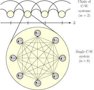
Figure 1: (Color online) A schematic graphical representation of the model. A chain of C-W models interacting within a certain range $w$ ($w=2$ in the figure). In the zoomed part the fully-connected structure of the single C-W model is shown. (Note that a connection between C-W models along the chain indicates connections between all spins contained in both models).

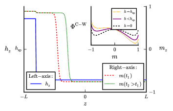
Figure 2: (Color online) A chain of coupled C-W systems. The external field is a function of position $z$: in the ‘seed’ region $h_{z}>h_{\mathrm{sp}}$, whilst in the bulk of the chain $h_{z}<h_{\mathrm{sp}}$. Starting every C-W system in the neighborhood of $m^{-}$, the composite system magnetizes according to a travelling wave that starts at the seed. Inset: the free energy of a C-W system in a uniform external field. In the so-called spinodal region, $0<h<h_{\mathrm{sp}}$, there are two minima $m^{-}$ and $m^{+}$, such that $\Phi^{\mathrm{C-W}}(m^{-})>\Phi^{\mathrm{C-W}}(m^{+})$. For $h>h_{\mathrm{sp}}$, $m^{+}$ is the only minimum of $\Phi^{\mathrm{C-W}}$.

IV Variational Bayes vs. Monte-Carlo

To solve the above inference problem we need to sample the posterior (Boltzmann) probability distribution (2) in order to compute its marginal probabilities (local magnetizations). The most commonly used methods for sampling fall into two classes: variational Bayes and Monte-Carlo (M-C). In this paper, we will mostly be concerned with the variational Bayes approach, as it is typically faster than M-C. However, since physicists are familiar with M-C, we will fist explain how the two approaches relate.

In physics, M-C is the ‘go-to’ method for minimizing the free energy in a spin system. Most generally, this involves constructing an algorithm that explores the parameter space and iteratively moves towards the state that minimizes the energy, subject to entropic constraints. The process is usually designed to be stochastic and Markovian. Some examples of famous Monte-Carlo Markov-Chain (MCMC) methods include the Metropolis-Hastings algorithm or the heat-bath algorithm. The upside of these approaches is that, in the limit of a large number of time steps, they are exact. However, the downside is that achieving such accuracy can be computationally expensive.

In terms of the limiting behavior of MCMC algorithms, we can persuade ourselves that if we define local magnetization averaged over realizations of the M-C dynamics as $m_{iz}^{t}=\langle s_{iz}^{t}\rangle_{\rm realization}$, then for the heat-bath algorithm with parallel update, the system evolves according to

$$m^{t+1}_{iz}=\tanh\left(\sum_{z^{\prime}\neq z}J_{zz^{\prime}}\sum_{j}m^{t}_{jz^{\prime}}+J_{zz}\sum_{j\neq i}m^{t}_{jz}+h_{z}\right)\,.$$ (10)

Where this expression can also be obtained by analyzing the M-C heat-bath dynamics in the limit $n=1$ and $w\rightarrow\infty$ (instead of $w$ finite and $n\rightarrow\infty$) de1994glauber . If one uses random sequential update in the M-C simulation, the behavior of the system in the large $N=n(2L+1)$ limit corresponds to the analogous differential equation

$$\frac{{\rm d}m_{iz}}{{\rm d}\tau}=\tanh\left(\sum_{z^{\prime}\neq z}J_{zz^{\prime}}\sum_{j}m_{jz^{\prime}}+J_{zz}\sum_{j\neq i}m_{jz}+h_{z}\right)-m_{iz}\,,$$ (11)

in terms of a rescaled time $\tau=t/N$.

In contrast to the above, the variational Bayes algorithm to compute the local marginals (magnetizations) uses the assumption that the posterior probability (Boltzmann) distribution can be written in a factorized form

$$P^{\rm MFT}_{N}({\bf s},h,J)=\prod_{i,z}\left[\frac{1+m_{iz}}{2}\delta_{s_{iz},1}+\frac{1-m_{iz}}{2}\delta_{s_{iz},-1}\right]$$ (12)

When this form is then substituted to the Kullback–Leibler divergence from $P^{\rm MFT}_{N}({\bf s},h,J)$ to $P_{N}({\bf s},h,J)$ we obtain the free energy

$$\begin{split}&F=-\sum_{\langle iz,jz^{\prime}\rangle}J_{zz^{\prime}}m_{iz}m_{jz^{\prime}}-\sum_{z}h_{z}\sum_{i}m_{i}\\ &+\sum_{iz}\left[\frac{1+m_{iz}}{2}\ln\left(\frac{1+m_{iz}}{2}\right)+\frac{1-m_{iz}}{2}\ln\left(\frac{1-m_{iz}}{2}\right)\right]\\ &=-\log{Z}+D_{\rm KL}(P^{\rm MFT}||P)\,.\end{split}$$ (13)

By imposing a stationarity condition on $F$ with respect to $m_{iz}$, we obtain the following fixed-point equation

$$m_{iz}=\tanh\left(\sum_{z^{\prime}\neq z}J_{zz^{\prime}}\sum_{j}m_{jz^{\prime}}+J_{zz}\sum_{j\neq i}m_{jz}+h_{z}\right)\,.$$ (14)

Solutions to this equation can be found, for instance, by iterating (10). So we see that for the C-W model, the evolution of the heat-bath MCMC is closely related to the variational Bayes inference. Indeed, it is also worth noting that, for the C-W model, the variational Bayes approach provides asymptotically exact values of the marginals (local magnetizations). For general inference problems no such algorithm exists, whilst for the two main motivational examples of this paper— LDPC codes and compressed sensing— the Bethe approximation (and a related belief propagation algorithm) is asymptotically exact.

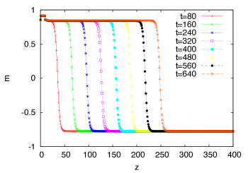
Figure 3: (Color online) The propagating wave obtained by iteration of Eq. (10) for the following parameters: $J=1.4$, $L=400$, $n=40$, $h=0.05$, $w=5$, $w_{\mathrm{seed}}=10$ and $h_{\mathrm{seed}}=0.3$.

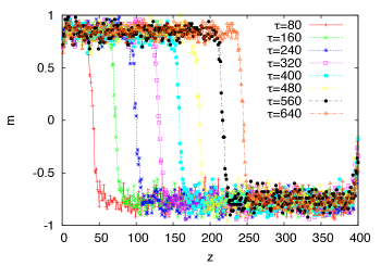
Figure 4: (Color online) The propagating wave obtained by Monte-Carlo heat-bath simulation for the following parameters: $J=1.4$, $L=400$, $n=100$, $h=0.05$, $w=5$, $w_{\mathrm{seed}}=10$ and $h_{\mathrm{seed}}=0.3$. Simulations were performed using random sequential update and therefore time must be rescaled by $\tau=t/N$.

As anticipated, iterating (10) (with appropriate parameter choices) results in a travelling wave of magnetization emanating from the seeded region, and eventually saturating the whole chain to the global optimum, $m^{+}$. As an example, in Fig. 3 we show the propagating wave for the following parameter values: $\,J=1.4\,,\,h=0.05\,,\,w=5\,,\,n=40\,,\,L=400$, where for this value of $J$, the field is below the spinodal point $h_{\rm sp}\approx 0.1518$. We initialize the whole system with local negative magnetization and on the first $w_{\mathrm{seed}}=10$ blocks we impose a seeding field $h_{\mathrm{seed}}=0.3$, which is above $h_{\rm sp}$. As can be seen in the figure, we observe the propagation of a magnetization wave.

So far, we have only discussed equations in terms of local magnetizations of a single spin variable. However, it is straightforward to see that, since we have no disorder, the local magnetization does not fluctuate from site-to-site within one block. We can therefore derive the equivalent of the ‘state’ or ’density’ evolution for the above algorithm by simply summing over $i$ on both sides of the equation, dividing by $n$, and then letting $n\rightarrow\infty$. In this way we obtain

$$m^{t+1}_{z}=\tanh\left(\sum_{z^{\prime}}D_{zz^{\prime}}m^{t}_{z^{\prime}}+Jm^{t}_{z}+h_{z}\right),$$ (15)

where

$$D_{zz^{\prime}}=J_{zz^{\prime}}-\delta_{z,z^{\prime}}J.$$ (16)

Here, it is helpful to make a few remarks: firstly, in the C-W model, the finite size fluctuations— neglected in (15)— are just a small (deterministic) correction to the fixed point values of the local magnetizations. This is different in more realistic problems like LDPC or compressed sensing where the disorder (either in the factor graph or in the measurement matrix) induces finite size effects that are not captured by the C-W model. Secondly, the free energy (13) can be minimized by iterative schemes other than (10), and also other MCMC algorithms lead to different evolution equations (10) with the same fixed point. For example, the Metropolis-Hastings MCMC with random sequential update is equivalent to

$$\frac{{\rm d}m_{z}}{{\rm d}\tau}=2e^{-\tilde{h}_{z}}\cosh\left(\tilde{h}_{z}\right)\left[\tanh\left(\tilde{h}_{z}\right)-m_{z}\right],$$ (17)

with

$$\tilde{h}_{z}=\sum_{z^{\prime}}D_{zz^{\prime}}m_{z^{\prime}}+Jm_{z}+h_{z}$$ (18)

in the large system-size limit. Whilst taking the steepest descent of the free energy (13) leads to

$$m_{z}^{t+1}=\sum_{z^{\prime}}D_{zz^{\prime}}m^{t}_{z^{\prime}}+Jm^{t}_{z}+h_{z}-{\rm atanh}(m^{t}_{iz})+m^{t}_{iz}.$$ (19)

In this paper, we pay specific attention to the most common update (10), but we stress that the same kind of analysis can be carried out for (17-19) and others.

V Continuous limit

Useful information about the behavior of the spatially coupled system can be understood if, following Urbankechains , we take the double limit $L\gg w\gg 1$, such that $L,w\rightarrow+\infty$ whilst $w/L\rightarrow 0$. In addition to this, introduce a space variable $x=z/w$ such that the limiting magnetization profile

$$\lim_{L,w\rightarrow+\infty:\ w/L\rightarrow 0}m_{wx}(\tau)\equiv m(x,\tau)\in[-1,+1],$$ (20)

is now a function of the continuous variables $x,\tau\in[-\infty,+\infty]$. In this limit, the sum over the kernel $D_{zz^{\prime}}$ becomes

$$\lim_{\begin{subarray}{c}w,L\rightarrow+\infty\\ w/L\rightarrow 0\end{subarray}}\sum_{z^{\prime}=-L}^{L}D_{zz^{\prime}}m_{z^{\prime}}(\tau)=\int_{-\infty}^{+\infty}\mathrm{d}x^{\prime}D\left(x^{\prime}\right)m(x-x^{\prime},\tau),$$ (21)

where $D\left(x\right)=J\left[g\left(|x|\right)-\delta\left(x\right)\right]$, and the right-hand side has been re-written using change of variable $x^{\prime}\mapsto x-x^{\prime}$. The state evolution equation (15) can then be written in the continuous limit as

$$\frac{\mathrm{d}m}{\mathrm{d}\tau}=\tanh\left(\left[D*m\right]+Jm+h\right)-m,$$ (22)

where the shorthand $[\cdot*\cdot]$ represents convolution and the explicit dependencies of $m(x,\tau)$ and $h(x)$ have been dropped. Notice that when $|x|\gg 1$, $D(x)=0$ and therefore in the convolution we can perform a gradient expansion. Due to symmetry, the lowest order term in the expansion with a non-zero contribution is quadratic. That is, the right-hand side of (21) is approximated by

$$\sim\left(\frac{J}{2}\int_{-\infty}^{+\infty}\mathrm{d}x^{\prime}g\left(|x^{\prime}|\right)x^{\prime 2}\right)\frac{\partial^{2}m}{\partial x^{2}}+\mathcal{O}(x^{3}).$$ (23)

Substituting into (22) and inverting the hyperbolic tangent then gives the result

$$\omega\frac{\partial^{2}m}{\partial x^{2}}=-Jm-h+{\rm atanh}\left(m+\frac{\partial m}{\partial\tau}\right)$$ (24)

where the pre-factor from (23) has been absorbed in the definition

$$\omega=\frac{J}{2}\int_{-\infty}^{+\infty}\mathrm{d}x^{\prime}g\left(|x^{\prime}|\right)x^{\prime 2}.$$ (25)

Working in this limit, it is now possible to look for traveling-wave solutions— that is, those of the form $m(x,\tau)=m(x-v\tau)$. This leads to an ordinary differential equation in terms of variable $y=x-v\tau$:

$$\omega\frac{\mathrm{d}^{2}m}{\mathrm{d}y^{2}}=-Jm-h+{\rm atanh}\left(m-v\frac{\mathrm{d}m}{\mathrm{d}y}\right).$$ (26)

If the bulk field $h$ is very small, the potential barrier between $m^{-}$ and $m^{+}$ is large and therefore $v$ is expected to be small too. The resulting expansion for $|v|\ll 1$ gives

$$\omega\frac{\mathrm{d}^{2}m}{\mathrm{d}y^{2}}\simeq\frac{\partial\Phi^{\mathrm{C-W}}(m)}{\partial m}-\frac{v}{1-m^{2}}\frac{\mathrm{d}m}{\mathrm{d}y}.$$ (27)

where $\Phi^{\mathrm{C-W}}$ is the free energy associated to the single C-W model, i.e., Eq. (13) for $L=0$. Multiplying both sides of this equation by $\mathrm{d}m(y)/\mathrm{d}y$, integrating over $y\in\mathbb{R}$, and applying the boundary conditions $m(-\infty)=m^{+}$, $m(+\infty)=m^{-}$, and $\mathrm{d}m(y)/\mathrm{d}y|_{y=-\infty}=\mathrm{d}m(y)/\mathrm{d}y|_{y=+\infty}=0$ implies that

$$v\simeq\Delta\Phi^{\mathrm{C-W}}/\gamma,$$ (28)

where the numerator $\Delta\Phi^{\mathrm{C-W}}$ is just the difference between the two minima of the C-W potential

$$\Delta\Phi^{\mathrm{C-W}}=\Phi^{\mathrm{C-W}}(m^{-})-\Phi^{\mathrm{C-W}}(m^{+}),$$ (29)

and the denominator $\gamma$ is given by

$$\gamma=\int_{-\infty}^{+\infty}\frac{\mathrm{d}y}{1-m^{2}(y)}\left[\frac{\mathrm{d}m(y)}{\mathrm{d}y}\right]^{2}.$$ (30)

An approximation for $\gamma$ that is consistent with a small $v$ assumption can be found by setting $v=0$ in (27). Once again multiplying both sides by $\mathrm{d}m(y)/\mathrm{d}y$, and this time integrating $y$ from $0$ to $Y$, the result is that

$$\frac{\omega}{2}\left[\frac{\mathrm{d}m(y)}{\mathrm{d}y}\right]^{2}\simeq\Phi^{\mathrm{C-W}}(m(y))-\Phi^{\mathrm{C-W}}(m^{-}),$$ (31)

where the aforementioned boundary conditions have been applied and $Y$ has been relabeled $y$. Substituting back into (30) gives

$$\gamma\simeq\int_{m^{-}}^{m^{+}}\frac{\mathrm{d}m}{1-m^{2}}\left\{\frac{2\left[\Phi^{\mathrm{C-W}}(m)-\Phi^{\mathrm{C-W}}(m^{+})\right]}{\omega}\right\}^{1/2}.$$ (32)

From (32) and (28) we can easily obtain an analytic formula for $v$ as a linear expansion in small $h$

$$v=\frac{(m^{+}_{0}-m^{-}_{0})}{\int_{m^{-}_{0}}^{m^{+}_{0}}\frac{\mathrm{d}m}{1-m^{2}}\left\{\frac{2\left[\Phi_{0}^{\mathrm{C-W}}(m)-\Phi_{0}^{\mathrm{C-W}}(m^{+}_{0})\right]}{\omega}\right\}^{1/2}}\,h$$ (33)

where the suffix ‘0’ refers to quantities at zero bulk field.

Note that this last Eq. (33) and the whole derivation of this Section is closely related to the description of flat moving interface in statistical physics of nucleation, see e.g., godreche1991solids . We also mention here that the steepest descent update (19) would lead to a different continuous equation, namely

$$\omega\frac{\partial^{2}m}{\partial x^{2}}=-Jm-h+{\rm atanh}\left(m\right)+\frac{\partial m}{\partial\tau},$$ (34)

that has the form of a bistable reaction-diffusion equation.

VI Front velocity as a function of the bulk field

We have already seen that one can calculate an approximation to the velocity of propagation of the wave— a proxy for the rate of convergence in inference— by taking an appropriate continuous limit and assuming $h$ to be small. However, it is helpful to know how good this approximation is, and indeed if there are any other factors that affect the relationship between $v$ and the bulk field $h$. (Recall that, in the analogy between the C-W model and generic inference problems, the value of $h$ represents a distance from the optimal setup).

VI.1 Large $w$, flat interaction.

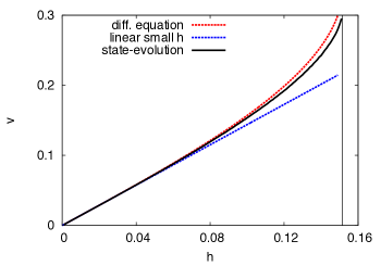
Figure 5: (Color online) The normalized velocity $v=\dot{z}/w$ as a function of the bulk field $h$ for $J=1.4$ computed in three different ways. The solid line is the ‘experimental’ speed measured in the iteration of Eq. (15) ($L=1000$, $w=30$), the dotted curved line is the speed determined through integration of Eq. (26) and the dotted straight line is given by the linearized analytic formula (33).

In Fig. 5, for the simplest case in which the function $g$ is a constant, we compare three different curves:

1. The velocity in the limit $n\gg L\gg w\gg 1$ as given by the ordinary differential equation (26). In order to obtain a (numerical) value for the propagation speed $v$ we integrate (26) between $-T$ and $T$ with $T\gg 1$, with an initialization $m(-T)=m^{+}$ and $m^{\prime}(-T)\approx 0$.

2. The velocity in the limit $n\gg L\gg w\gg 1$ as calculated from the analytic linearized formula given in Eq. (33).

3. The velocity computed from numerical iteration of the asymptotic update (15) at finite length $L=1000$, and finite interaction range $w=30$. In this case, we only use parameter values that lead to wave propagation (propagation/non-propagation conditions will be discussed in the next Section). Note that, given that the wave propagates, its speed (in the bulk) is independent (within the numerical precision) of the seed.

The main result here is that, as expected, the asymptotic update equation in the continuous limit gives a good estimate for values of the field not too close to the spinodal point. Indeed, both results are bounded from below by the analytical form (33), valid for sufficiently small $h$.

VI.2 Large $w$, different shapes of the interaction.

So far, our analysis has only considered one type of interaction, that gives equal weights to all neighbors in a certain range— i.e., $g$ is a ‘tophat’ function. In fact, the velocity of the front can be increased by changing the ‘shape’ of this interaction such that the coupling is strongest between blocks that are furthest away (but still bounded by the limits of the interaction range $w$). In order to show this, consider the generalized form

$$g(x)=\left\{\begin{array}[]{cl}0&\mathrm{if}\ |x|>1\\ f(x)\left[\int_{-1}^{1}f(x){\rm d}x\right]^{-1}&\mathrm{if}\ |x|\leq 1\end{array}\right.,$$ (35)

where now $f$ can be any symmetric function. To demonstrate the effect of $f$, Fig. 6 shows the velocity computed by integrating (26) for three different forms: $f\sim\mathrm{constant}$ (tophat), $f\sim 1+x^{2}$ (parabolic) and $f\sim 1+x^{4}$ (quartic). In the inset of Fig. 6, we also show the full dependence of the speed on the constant $\omega$— Eq. (25)— for a given value of the bulk field. Indeed, from Eq. (33), we see explicitly that, in the regime in which the linearization is a consistent approximation, $v\sim\sqrt{\omega}$.

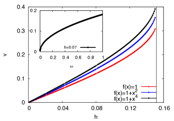
Figure 6: (Color online) [Main frame] The normalized velocity $v=\dot{z}/w$ as a function of the bulk field $h$ with $J=1.4$ for the three model variants described in the main text. From bottom to top: tophat interaction, quadratic interaction and quartic interaction. [Inset] The speed computed by integration of Eq. (24) for fixed bulk field $h=0.07$ and varying $\omega$.

It is important to stress at this point that changing $\omega$ is the only tool that we have to truly maximize the speed (in terms of ‘physical time’). To see this, suppose that we are at fixed chain length $L$, block spins $n$, bulk field $h$, and our unit of time is the single iteration over the whole system. We have already stated that, once propagation is achieved, the speed is proportional to $w$ and independent of the shape and extent of the seed. On the other hand, the single iteration takes a time which is linear in $n$, $L$ and $w$, therefore changing the interaction range has no effect on the speed in terms of real time and the only effect on the physical speed is given by the shape of the interaction, which in turn determines the value of $\omega$.

VI.3 Finite $w$ effects.

Until this point we have only considered parameter values that are close to the continuous limit— i.e., $L\gg w\gg 1$. However, as will become clear in the following Section, the case of small $w$ is very relevant for practical implementations of spatial coupling. Indeed, in previous work Urbankechains , it has been shown that small oscillations in the Van der Waals curve mean that propagation can only be formally proved for $w\gg 1$. However, simulations indicate that the reality of the situation is much more positive, and small values of $w$ might be practical in many situations.

The authors of Urbankechains consider the global average magnetization along the chain, namely

$$m=\frac{1}{2L+1}\sum_{z=-L}^{L}m_{z}$$ (36)

and show that the propagation of the wave (regardless of the seeding scheme) is subject to the constraint that the free energy has non-positive derivative with respect to $m$ between the two uniform states $m^{-}_{0}$ and $m^{+}_{0}$— the negative and positive equilibrium states respectively of the uncoupled C-W model at $h=0$. With uniform interaction, $J>1$, and small magnetic field, the derivative of the free-energy reads Urbankechains

$$C(w,J)\,e^{-\frac{\pi^{2}w}{Jm_{0}^{+}}}\sin\left(2\pi\frac{m}{m_{0}^{+}}L\right)-h$$ (37)

where $C(w,J)$ is a pre-factor that can be computed. This means that we need (regardless of the seeding conditions)

$$h\geq A_{w}\equiv C(w,J)\,e^{-\frac{\pi^{2}w}{Jm^{0}_{+}}}$$ (38)

for the derivative to be negative everywhere and propagation to be possible. In fact, the authors of Urbankechains evaluated the amplitude $A_{w}$ of the oscillation for $J=1.4$ in their Table 2, and for $w=1$ they find $A_{1}=2.2\times 10^{-5}$. In Fig. 7 we show the speed of the wave for $J=1.4$ at very weak bulk field with ideal seeding conditions (i.e., we fix half of the chain to positive magnetization). We see that at small bulk field $h<A_{w}$ the velocity is zero, is agreement with the theory of Urbankechains . However, more broadly, it is clear that this effect is observable only at extremely small magnetic fields, even for $w=1$. Furthermore, the effect decreases exponentially with the value of $w$. We therefore conclude that these oscillations are not likely to cause problems in practical implementations of spatial coupling.

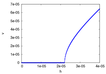
Figure 7: (Color online) The normalized velocity as a function of the bulk field $h$ for spatially coupled system with interaction range $w=1$. For bulk fields smaller than the critical value $h<A_{1}$ the wave does not propagate.

VII The role of the termination condition

As discussed in the Introduction, the majority of existing studies regarding wave propagation in spatially coupled systems consider initial conditions analogous to $m(-\infty)=m^{+}$, $m(+\infty)=m^{-}$, and $\mathrm{d}m(y)/\mathrm{d}y|_{y=-\infty}=\mathrm{d}m(y)/\mathrm{d}y|_{y=+\infty}=0$. In real inference problems however, there is no way of fixing such an initial condition and instead the propagation of the wave has to be enforced by a proper termination condition— i.e., a ‘seed’, as introduced in Sec. III. In this Section we analyze the properties of the seed under which a travelling wave starts to propagate in the system, and we discuss how to optimize its cost (corresponding to the rate loss in coding).

VII.1 Conditions for propagation

The travelling wave will start to propagate in the spatially coupled system only if the size of the seed ($w_{\rm seed}$) and the strength of the seed ($h_{\rm seed}$) are both large enough. Indeed, the propagation/non-propagation boundary can be plotted as a function of (normalized) variables $h_{\mathrm{seed}}/h_{\rm sp}$ and $w_{\mathrm{seed}}/w$ (see Fig. 8).

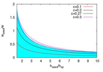
Figure 8: (Color online) The threshold between propagation and non-propagation for $J=1.4$, $w=60$ and $h=0.05$ given by the state evolution, Eq. (15). Cyan (light grey) represents region of parameters where the wave does not propagate and white represents a region where it does propagate. The dotted lines superimposed to the shading are cost-density isolines, defined by Eq. (39), for different values of $c$.

When designing the spatially coupled system, our main objective is to obtain propagation of the magnetization wave while keeping the average magnetic field on the chain as close as possible to the bulk field $h$— i.e., the goal is to minimize the cost

$$\begin{split}{\cal C}&=h_{\rm av}-h=w_{\mathrm{seed}}\frac{h_{\mathrm{seed}}-h}{2L+1}=\\ &=\frac{w}{2L+1}c\left(\frac{w_{\mathrm{seed}}}{w},\frac{h_{\mathrm{seed}}}{h_{\rm sp}}\right),\end{split}$$ (39)

which is analogous to the rate loss in error-correcting codes, for example. Here, $c$ is a ‘cost density’, and is a function of rescaled variables. This means that for a given choice of the chain-length and interaction range, the cost-density isolines can be superimposed in rescaled variables. As can be seen in Fig. 8, all but one of the isolines cross the threshold line twice. Given $w$ and $L$ fixed then, the best choice of parameters is defined as the point where the unique cost isoline and the threshold line meet tangentially. In Fig. 9 we show how $c$ varies on the threshold line as parametrized by $h_{\mathrm{seed}}/h_{\rm sp}$ and $w_{\mathrm{seed}}/w$. From this it is clear that there is indeed a choice that corresponds to minimal cost.

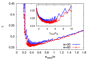
Figure 9: [Main Frame] (Color online) The cost-density along the threshold line in Fig. 8 as a function of the ratio $w_{\mathrm{seed}}/w$, for $w=30$ and $w=60$. [Inset] (Color online) The cost-density along the threshold line in Fig. 8 as a function of the seeding field, for $w=30$ and $w=60$. In both cases, the plots tend to smooth curve, independent of $w$, for $w\gg 1$.

Fig. 9 shows explicitly that the cost density curve along the threshold line tends towards being independent of $w$ at large values $w$. In other words, for $w\gg 1$, the cost of achieving propagation depends only on the ratio $w_{\mathrm{seed}}/w$ and not on $w$ itself. This kind of analysis gives more insight in the choice of parameters that achieve propagation minimizing the ‘field loss’ (or rate loss in the case of coding theory), and can function as a guide in practical code implementations when $w$ is large.

VII.2 Termination cost at small $w$

Analysis of the previous section is not valid for small $w$, when the effect of the intrinsic discreteness of the system is strong. At the same time the total cost, eq. (39), is linearly dependent on the range $w$, consequently it seems important to evaluate the cost at small values of $w$. In this Section we hence consider the typical case of a chain of length $L=500$ with $J=1.4$ and small values of the interaction range $w$. Making use of the state evolution (15) we study what is the minimal cost for propagation as a function of the bulk field for different values of $w$.

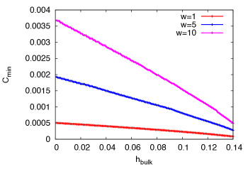
Figure 10: (Color online) The minimal cost as a function of the bulk field for $L=500$, $J=1.4$ and different values of the interaction range. In particular, from bottom to top, $w=1$, $w=5$ and $w=10$.

As can be seen from Fig. 10 the minimal total cost is reached for $w=1$ and an appropriate choices of the seeding parameters (see Fig. 11). These two figures leads us to a perhaps unexpected conclusion that the optimized seeding condition uses range of interactions $w=1$ with seed size $w_{\rm seed}=1$ and sufficiently large $h_{\rm seed}$ (as specified in Fig. 11).

Figure 11: (Color online) With the same parameters as Fig. 10, the three curves represent the seeding field that minimizes the cost as a function of the bulk field. The superimposed numbers are the values of the seeding range $w_{\rm seed}$ corresponding to the minimum (shown only for $w=1$ and $w=5$).

VIII Conclusions

In this paper we have evaluated several properties of the spatially coupled C-W model. We reached the following interesting conclusions:

• The speed of propagation of the travelling wave can be increased by choosing interaction profile that has a large variance.

• The interaction range $w$ does not really need to be large, since the negative effects associated with finite $w$ are only visible at extremely small values of the magnetic field (even for $w=1$). Indeed, in practical situations, both the measurement noise and finite size effects will play an important role, which makes such small values of the external field— i.e., such that the effects of finite $w$ are felt— unfeasible.

• In order to minimize the termination cost (or in coding language, the rate loss) the optimal parameters are: an interaction range $w=1$, seed size $w_{\rm seed}=1$, and values of the seeding field $h_{\rm seed}$ summarized in Fig. 11.

In future work we need to clarify whether the above conclusions are particular to a chain of C-W models, or whether they apply universally to other spatially coupled systems.

One important aspect that the coupled C-W model is missing are non-trivial finite size effects. Indeed, the C- W model does not have any disorder and hence there is a very little difference between the state evolution and the real evolution in a system of finite size. This will be different in interesting applications of spatially coupled systems and needs to be evaluated.

- [1] D. L. Donoho. Compressed sensing. IEEE Trans. Inform. Theory, 52:1289, 2006.
- [2] Tom Richardson and Rüdiger Urbanke. Modern Coding Theory. Cambridge University Press, 2008.
- [3] M. Mézard and A. Montanari. Information, Physics, and Computation. Oxford Press, Oxford, 2009.
- [4] F. Krzakala, M. Mézard, F. Sausset, Y.F. Sun, and L. Zdeborová. Statistical physics-based reconstruction in compressed sensing. Phys. Rev. X, 2:021005, 2012.
- [5] Claude Elwood Shannon. A mathematical theory of communication. ACM SIGMOBILE Mobile Computing and Communications Review, 5(1):3–55, 2001.
- [6] A. J. Felstrom and K.S. Zigangirov. Time-varying periodic convolutional codes with low-density parity-check matrix. IEEE Trans. Inf. Theory, 45(6):2181 –2191, 1999.
- [7] Michael Lentmaier, Arvind Sridharan, K Sh Zigangirov, and DJ Costello. Terminated ldpc convolutional codes with thresholds close to capacity. In Proceedings of International Symposium on Information Theory, ISIT 2005, pages 1372–1376. IEEE, 2005.
- [8] Michael Lentmaier, Arvind Sridharan, Daniel J Costello, and K Sh Zigangirov. Iterative decoding threshold analysis for ldpc convolutional codes. IEEE Trans. Inf. Theory, 56(10):5274–5289, 2010.
- [9] Shrinivas Kudekar, Thomas J Richardson, and Rüdiger L Urbanke. Threshold saturation via spatial coupling: Why convolutional ldpc ensembles perform so well over the bec. IEEE Transactions on Information Theory, 57(2):803–834, 2011.
- [10] Shrinivas Kudekar, Tom Richardson, and Rudiger Urbanke. Spatially coupled ensembles universally achieve capacity under belief propagation. In Proc. of the IEEE Int. Symposium on Information Theory (ISIT), pages 453–457, 2012.
- [11] D. L. Donoho, A. Javanmard, and A. Montanari. Information-theoretically optimal compressed sensing via spatial coupling and approximate message passing. In Proc. of the IEEE Int. Symposium on Information Theory (ISIT), pages 1231–1235, 2012.
- [12] Christian Schlegel and Dmitri Truhachev. Multiple access demodulation in the lifted signal graph with spatial coupling. In IEEE International Symposium on Information Theory Proceedings (ISIT), pages 2989–2993. IEEE, 2011.
- [13] Keigo Takeuchi, Toshiyuki Tanaka, and Tsutomu Kawabata. Improvement of bp-based cdma multiuser detection by spatial coupling. In IEEE International Symposium on Information Theory Proceedings (ISIT), pages 1489–1493. IEEE, 2011.
- [14] Pan Zhang, Florent Krzakala, Marc Mézard, and Lenka Zdeborová. Non-adaptive pooling strategies for detection of rare faulty items. arXiv preprint arXiv:1302.0189, 2013.
- [15] S Hamed Hassani, Nicolas Macris, and Ruediger Urbanke. Chains of mean-field models. J. Stat. Mech.: Theor. and Exp., page P02011, 2012.
- [16] Arvind Yedla, Yung-Yih Jian, Phong S Nguyen, and Henry D Pfister. A simple proof of threshold saturation for coupled scalar recursions. In 7th International Symposium on Turbo Codes and Iterative Information Processing (ISTC), pages 51–55, 2012.
- [17] Shrinivas Kudekar, Tom Richardson, and Ruediger Urbanke. Wave-like solutions of general one-dimensional spatially coupled systems. arXiv preprint arXiv:1208.5273, 2012.
- [18] Vahid Aref, Laurent Schmalen, and Stephan ten Brink. On the convergence speed of spatially coupled ldpc ensembles. arXiv preprint arXiv:1307.3780, 2013.
- [19] Shrinivas Kudekar, Cyril Measson, Tom Richardson, and R Urbankez. Threshold saturation on bms channels via spatial coupling. In Turbo Codes and Iterative Information Processing (ISTC), 2010 6th International Symposium on, pages 309–313. IEEE, 2010.
- [20] Pablo M Olmos and Rüdiger Urbanke. Scaling behavior of convolutional ldpc ensembles over the bec. In IEEE International Symposium on Information Theory Proceedings (ISIT), pages 1816–1820. IEEE, 2011.
- [21] Pablo M Olmos, Fernando Perez-Cruz, Luis Salamanca, and Juan Jose Murillo-Fuentes. Finite-length performance of spatially-coupled ldpc codes under tep decoding. In IEEE Information Theory Workshop (ITW), pages 492–496. IEEE, 2012.
- [22] Pablo M Olmos, David G. M. Mitchell, Dmitri Truhachev, and Daniel J. Costello. A finite length performance analysis of ldpc codes constructed by connecting spatially coupled chains. In IEEE Information Theory Workshop (ITW), 2013.
- [23] A De Masi, Enza Orlandi, Errico Presutti, and Livio Triolo. Glauber evolution with kac potentials. i. mesoscopic and macroscopic limits, interface dynamics. Nonlinearity, 7(3):633, 1994.
- [24] Claude Godrèche. Solids far from Equilibrium, volume 1. Cambridge University Press, 1991. Chapter 3 by J. Langer: An introduction to kinetics of first-order phase transition.