Various methods of optimizing control pulses for quantum systems with decoherence

Abstract

We study three methods of obtaining an approximation of unitary evolution of a quantum system under decoherence. We use three methods of optimizing the control pulses: genetic optimization, approximate evolution method and approximate gradient method. To model the noise in the system we use the Lindblad equation. We obtain results showing that genetic optimization may give a better approximation of a unitary evolution in the case of high noise.

I Introduction

One of the fundamental issues of quantum information science is the ability to manipulate the dynamics of a given complex quantum system. Since the beginning of quantum mechanics, controlling a quantum system has been an implicit goal of quantum physics, chemistry and implementations of quantum information processing Cheng et al. (2005).

If a given quantum system is controllable, i.e. it is possible to drive it into a previously fixed state, it is desirable to develop a control strategy to accomplish the required control task. In the case of finite dimensional quantum systems the criteria for controllability can be expressed in terms of Lie-algebraic concepts Albertini and D’Alessandro (2002); Elliott (2009); d’Alessandro (2008). These concepts provide a mathematical tool, in the case of closed quantum systems, i.e. systems without external influences.

It is an important question whether the system is controllable when the control is performed only on a subsystem. This kind of approach is called a local-controllability and can be considered only in the case when the subsystems of a given system interact. As examples may serve coupled spin chains or spin networks d’Alessandro (2008); Burgarth and Giovannetti (2007); Burgarth et al. (2009); Puchała (2012). Local-control has a practical importance in proposed quantum computer architectures, as its implementation is simpler and the effect of decoherence is reduced by decreased number of control actuators Montangero et al. (2007); Fisher et al. (2010).

A widely used method for manipulating a quantum system is a coherent control strategy, where the manipulation of the quantum states is achieved by applying semi-classical potentials in a fashion that preserves quantum coherence. In the case when a system is controllable it is a point of interest what actions must be performed to control a system most efficiently, bearing in mind limitations imposed by practical restrictions Morzhin (2012); Dominy et al. (2013); Qi (2013); Pawela and Puchała (2014, 2013). The always present noise in the quantum system may be considered as a such constrain Li et al. (2009); Khodjasteh et al. (2010); Schmidt et al. (2011); Gawron et al. (2014); Schulte-Herbrüggen et al. (2011); Hwang and Goan (2012); Clausen et al. (2012); Floether et al. (2012). Therefore it is necessary to study methods of obtaining piecewise constant control pulses which implement the desired quantum operation on a noisy system.

In this paper we present a general method of obtaining a piecewise-constant controls, which is robust with respect to noise in the quantum system. This means, we wish to perform a unitary evolution on a greater system than the target one, and discard the ancilla.

This paper is organized as follows. In Section II we introduce the model of the studied quantum system. Section III shows different approaches to solving the Lindblad equation. Next, in Section III.3 we introduce genetic programming. Detailed description of the optimization procedure and studied cases can be found in Section III.3.3. In Section IV we show results of the numerical simulations. Finally, we summarize this work in Section V.

II Model of the quantum system

Our goal is to implement the unitary operations $U_{\mathrm{NOT}}=\sigma_{x}\otimes{\rm 1l}$ and $U_{\mathrm{SWAP}}={\rm 1l}\otimes\sum_{ij}|i\rangle\langle j|\otimes|j\rangle\langle i|$ on a quantum system modeled as a an isotropic Heisenberg spin-$1/2$ chain of a finite length $N$. We will study two and three qubit systems. The total Hamiltonian of the aforementioned quantum control system is given by

$$H(t)=H_{0}+H_{c}(t),$$ (1)

where

$$H_{0}=J\sum_{i=1}^{N-1}S_{x}^{i}S_{x}^{i+1}+S_{y}^{i}S_{y}^{i+1}+S_{z}^{i}S_{z}^{i+1},$$ (2)

is a drift part given by the Heisenberg Hamiltonian. The control is performed only on the $n^{\textrm{th}}$ spin and is Zeeman-like, i.e.

$$H_{c}(t)=h_{x}(t)S_{x}^{n}+h_{y}(t)S_{y}^{n}.$$ (3)

In the above $S_{k}^{i}$ denotes $k^{\text{th}}$ Pauli matrix acting on the spin $i$. Time dependent control parameters $h_{x}(t)$ and $h_{y}(t)$ are chosen to be piecewise constant. For notational convenience, we set $\hbar=1$ and after this rescaling frequencies and control-field amplitudes can be expressed in units of the coupling strength $J$, and on the other hand all times can be expressed in units of $1/J$ Heule et al. (2010).

We model the noisy quantum system using the Markovian approximation with the master equation in the Kossakowski-Lindlbad form

$$\frac{\mathrm{d}\rho}{\mathrm{d}t}=-\mathrm{i}[H(t),\rho]+\sum_{j}\gamma_{j}(L_{j}\rho L_{j}^{\dagger}-\frac{1}{2}\{L_{j}^{\dagger}L_{j},\rho\}),$$ (4)

where $L_{j}$ are the Lindblad operators, representing the environment influence on the system Nielsen and Chuang (2000) and $\rho$ is the state of the system.

The main goal of this paper is to compare various methods for optimizing control pulses $h_{x}(t),h_{y}(t)$ for the model introduced above. In the next section we present three methods for this purpose. The comparison of the control pulses obtained by different methods is done by applying these pulses into the above model and analysis of the obtained results.

III Various approaches to fidelity maximization

In this Section we describe three methods we used to Obtain optimal control pulses. The first method is an approximate method for obtaining a mapping which is close to a unitary one. The second uses an approximate derivative of the mapping with respect to control pulses. Both of these methods allows to compute approximate gradient of the fitness function. In our numerical research we perform optimization with use of the L-BFGS-B optimization algorithm Zhu et al. (1997). This algorithm requires efficient gradient computation. Its main advantages lies in harnessing the approximation of Hessian of fitness function (we refer to the section 3 of Byrd et al. (1995) for details). Finally, we use genetic programming to optimize control pulses without the need for computing gradient of the fidelity function.

III.1 Approximate method

Assuming piecewise constant control pulses the Hamiltonian in Eq. (4) becomes independent of time during the duration of the pulse. This allows us to simplify the master equation.

For notational convenience, let us write the decoherence part of the Eq. (4) in the following form Havel (2003)

$$-\mathcal{G}=\sum_{j}\gamma_{j}\left(L_{j}\otimes\overline{L_{j}}-\frac{1}{2}\left[\left(L_{j}^{\dagger}L_{j}\right)\otimes{\rm 1l}+{\rm 1l}\otimes\left(\overline{L_{j}^{\dagger}L_{j}}\right)\right]\right).$$ (5)

The second term in Eq. 4 can be written as

$$\mathrm{i}\mathcal{H}=\mathrm{i}\left({\rm 1l}\otimes\overline{H}-H\otimes{\rm 1l}\right).$$ (6)

This observations allow us to write a mapping representing the evolution of a system in an initial state $\rho$ under Eq. (4) for time $t$ as

$$A=\exp(-t\mathcal{F}),$$ (7)

where $-\mathcal{F}=-\mathcal{G}-\mathrm{i}\mathcal{H}$. The final state of the evolution is

$$\mathrm{res}(\rho_{f})=A\mathrm{res}(\rho),$$ (8)

where $\mathrm{res}(\cdot)$ is a linear mapping defined as

$$\mathrm{res}(|\phi\rangle\langle\psi|)=|\phi\rangle|\psi\rangle.$$ (9)

We can approximate the superoperator $A$ as

$$\begin{split}A\approx&\\ &\exp\left[-\frac{1}{2}t\sum_{j}\left(L_{j}^{\dagger}L_{j}\right)\otimes{\rm 1l}+{\rm 1l}\otimes\left(\overline{L_{j}^{\dagger}L_{j}}\right)\right]\times\\ \times&\exp\left(t\sum_{j}L_{j}\otimes\overline{L_{j}}\right)\times\exp\left(-t\mathrm{i}\mathcal{H}\right)+O(t^{2})\\ =&\mathcal{A}(t)\mathcal{B}(t)\mathcal{C}(t)+O(t^{2}).\end{split}$$ (10)

Note that, only the $\mathcal{C}(t)$ term depends on the control pulses. Assuming piecewise constant control pulses, we can write the resulting superoperator as

$$A=\prod_{i=1}^{n}\mathcal{A}(\Delta t_{i})\mathcal{B}(\Delta t_{i})\mathcal{C}(\Delta t_{i}),$$ (11)

where $n$ is the total number of control pulses and $\Delta t_{i}$ is the length of the time interval in which control pulse $h_{i}$ is applied to the system. The derivative of the superoperator with respect to a control pulse $h_{l}$ is

$$\begin{split}\frac{\partial A}{\partial h_{l}}=&\left(\prod_{i=1}^{l-1}\mathcal{A}(\Delta t_{i})\mathcal{B}(\Delta t_{i})\mathcal{C}(\Delta t_{i})\right)\times\\ \times&\left(\mathcal{A}(\Delta t_{l})\mathcal{B}(\Delta t_{l})\frac{\partial\mathcal{C}(\Delta t_{l})}{\partial h_{l}}\right)\times\\ \times&\left(\prod_{i=l+1}^{n}\mathcal{A}(\Delta t_{i})\mathcal{B}(\Delta t_{i})\mathcal{C}(\Delta t_{i})\right),\end{split}$$ (12)

We use the fidelity as the figure of merit

$$f=\frac{1}{2^{2N}}\Re(\mathrm{Tr}A_{\mathrm{T}}^{\dagger}A),$$ (13)

where $N$ is the number of qubits in the system and $A_{\mathrm{T}}$ is the target superoperator. The derivative of the fidelity is given by

$$\frac{\partial f}{\partial h_{l}}=\frac{1}{2^{2N}}\Re\left(\mathrm{Tr}\left(A_{\mathrm{T}}\frac{\partial A}{\partial h_{l}}\right)\right).$$ (14)

III.2 Approximate gradient method

In this section we follow the results by Machnes et. al. Machnes et al. (2011). In order to introduce the approximate gradient method, we introduce the following notation

$$\hat{H}(\cdot)=[H(t),\cdot].$$ (15)

This allows us to write Eq. (4) in the form

$$\frac{\partial\rho}{\partial t}=-(\mathrm{i}\hat{H}+\mathcal{L})\rho(t).$$ (16)

The evolution of a quantum map under these equation is given by

$$\frac{\partial X(t)}{\partial t}=-(\mathrm{i}\hat{H}+\mathcal{L})X(t).$$ (17)

In order to perform numerical simulations, Eq. (17) needs to be discretized. Given a total evolution time $T$, we divide it into $M$ small intervals, each of length $\Delta t=T/M$. Hence, the quantum map in the $k^{\mathrm{th}}$ time interval is given by

$$X_{k}=\exp\left[-\Delta t(\mathrm{i}\hat{H}(t_{k})+\mathcal{L}(t_{k}))\right].$$ (18)

We utilize the trace fidelity as the figure of merit for this optimization problem

$$f=\frac{1}{2^{2N}}\Re\mathrm{Tr}\left[X^{\dagger}_{\mathrm{target}}X(T)\right]=\frac{1}{2^{2N}}\Re\mathrm{Tr}\left[\Lambda^{\dagger}(t_{k})X(t_{k})\right],$$ (19)

where $X(t_{k})=X_{k}X_{k-1}\cdots X_{1}X_{0}$ and $\Lambda^{\dagger}(t_{k})=X^{\dagger}X_{M}X_{M-1}\cdots X_{k+2}X_{k+1}$. This allows us to write the derivative of the fidelity with respect to the control pulses as

$$\frac{\partial f}{\partial h_{j}(t_{k})}=\frac{1}{2^{2N}}\Re\mathrm{Tr}\left[\Lambda^{\dagger}(t_{k})\left(\frac{\partial X_{k}}{\partial h_{j}(t_{k})}\right)X(t_{k-1})\right].$$ (20)

Since $\mathcal{L}$ and $\mathrm{i}\hat{H}$ need not commute, we can not calculate the derivative $\frac{\partial X_{k}}{\partial h_{j}(t_{k})}$ using exact methods. The best approach is to use the following approximation for the gradient

$$\frac{\partial X_{k}}{\partial h_{j}(t_{k})}\approx-\Delta t\left(\mathrm{i}\hat{H}+\frac{\partial\mathcal{L}(h_{j}(t_{k}))}{\partial h_{j}(t_{k})}\right)X_{k}.$$ (21)

This approximation is valid provided that

$$\Delta t\ll\frac{1}{||\mathrm{i}\hat{H}+\mathcal{L}||_{2}}.$$

III.3 Genetic programming

Genetic programming (GP) is a numerical method based on the evolutionary mechanisms Spector (2004); Gepp and Stocks (2009). There are two main reasons for using GP for finding optimal control pulses. First of all it enables to perform numerical search in complicated, mathematically untraceable space. On the other hand, one should note that the values of control pulses in different time intervals can be set independently. Thus the idea of genetic code fits well as a model for a control setting. Thanks to such an representation, genetic programming enables to exchange values of control pulses in some fixed intervals between control settings that results with maximally accurate approximation of the desired evolution.

III.3.1 General GP algorithm

Genetic programming belongs to the family of search heuristics inspired by the mechanism of natural evolution. Each element of a search space being candidate for a solution is identified with a representative of a population. Every member of a population has its unique genetic code, which is its representation in optimization algorithm. In most of the cases genetic code is a sequence of values from a fixed set $\Sigma$ of possible values of all the features that characterize a potential solution $x\in\Sigma^{n}$ in the search space. Searching for the optimal solution is done by the systematic modification and evaluation of genetic codes of population members due to the rules of the evolution such as mutation, selection, crossover and inheritance.

Mutators are functions that change single elements of a genetic code randomly. A basic example of a mutator is a function that randomly changes values of a representative $x$ at all positions with some non-zero probability

$$M(x)_{i}=\left\{\begin{array}[]{cc}x_{i},&\mathrm{probability}\hskip 2.84544ptp\\ \mathrm{rand}(\Sigma),&\mathrm{probability}\hskip 2.84544pt1-p\end{array}\right..$$ (22)

Crossovers implement the mechanism of inheritance. This function divides given parental genetic code and create a new genetic code. Commonly two new codes are created at the same time from two parental codes. An example of such crossover is so called two point cut, where both parental codes ($x_{i},y_{i}$) are cut into three regions and the middle segments are interchanged

$$x^{\prime}_{i}=\left\{\begin{array}[]{cc}x_{i}&i\leq c_{1}\lor c_{2}\leq i\\ y_{i}&c_{1}<i<c_{2}\end{array}\right.,\hskip 14.22636pty^{\prime}_{i}=\left\{\begin{array}[]{cc}x_{i}&c_{1}<i<c_{2}\\ y_{i}&i\leq c_{1}\lor c_{2}\leq i\end{array}\right.,$$ (23)

where $c_{1}<c_{2}$ are randomly chosen indices. In every iteration of the algorithm all members of the population are evaluated using fitness function $f:\Sigma^{n}\to\Re$ which enables elements ordering. Then, using a selector function, the set of the best members is obtained and used to create a new generation of the population using mutation and crossover functions. There is a number of strategies for defining selector function – from completely random choices to the deterministic choice of best representatives.

Strategy based on evolution mechanism makes genetic programming especially usable when parts of genetic code represent features of elements of a search space that can be interchanged between elements independently. In such case GA is expected to find the features that occur in well fitted representatives and mix them in order to find the best possible combination. Pseudo code representing this approach is presented in Listing 1.

population = RandomPopulation()
for( generationsNumber ){
    newPopulation = []
    for(i = 0; i<population.size()/2; i++){
        mom = Selector(population)
        dad = Selector(population)
        (sister, brother) = CrossOver(mom, dad)
        Mutator(sister)
        Mutator(brother)
        newPopulation.append(sister)
        newPopulation.append(brother)
    }
    population = newPopulation
}

Listing 1: Pseudo code representing the algorithm of genetic programming. Functions Selector, Mutator and CrossOver work as defined in Section III.3.

While the customization of population representation and fitness function unavoidably relies on the optimization problem, other parameters of genetic programming such as crossover and mutation methods are universal.

III.3.2 Customization of the GP

Using GP schema requires obtaining proper representation of a problem. First of all one need to model the space of possible solutions as a set of genomes, usually by representing each of unique and independent features of a solution as one gene. Secondly, it is necessary to define a fitness function that allows to estimate genomes in a way that is consistent with the optimization problem. Using this function one need to determine selection method. The last step is to define methods for modifying modeled genomes. It may be methods based on mutation, crossing-over or both.

In this work we investigate methods for optimizing the sequence of control pulses in order to perform given unitary evolution. As we assume that control pulses in each time step are independent, it is a natural to define each of subsequent control pulses as gene. In this case genome is modeled as sequence od real numbers. It is a very convenient method, because there are many already developed mutation and crossing-over methods for such genome model that have been successfully applied to the problems of searching for the optimal evolution Goldberg (1989); Sadowski (2013). Methods of selection do not depend on genome model and can be based on a variety of already existing ones as well.

Since GP schema does not require the ability to compute gradient of considered fitness function one can use any method for genome estimation. In this work we use control pulses represented by given genome to perform simulation of the system evolution and obtain resulting state that is compared with the one resulting from target evolution. For comparison purposes we apply functions described in section III.3.3.

III.3.3 Optimization

In order to optimize a controlled evolution of a system governed by the Lindblad equation, we perform optimization of the average of distances between target state operator and the resulting states for each basis matrix of the space of input states. Our fitness function is defined as

$$f([c_{0},...,c_{M}])=\frac{1}{2^{2N}}\sum_{i=1}^{2^{2N}}\mathrm{Tr}\rho^{i}_{\mathrm{T}}\mathrm{Tr}_{A}\left(\Phi(\rho^{i}_{0},[c_{0},...,c_{M}])\right),$$ (24)

where $\mathrm{Tr}_{A}$ denotes tracing out the ancila, $N$ is the total number of qubits in the system, $\rho^{i}_{0}$ denotes the $i^{\mathrm{th}}$ basis matrix, $\rho_{\mathrm{T}}^{i}=U_{\mathrm{T}}\mathrm{Tr}_{A}(\rho_{0}^{i})U_{\mathrm{T}}^{\dagger}$ is the target density matrix and $\Phi$ is the quantum channel corresponding to the time evolution of $\rho_{0}^{i}$ under Eq. (4) for control pulses $[c_{0},...,c_{M}]$.

We study two noise models, the amplitude damping and phase damping noise. The former is given by the Lindblad operator $L_{1}=\sigma_{-}=|0\rangle\langle 1|$, while the latter is $L_{2}=\sigma_{z}$.

IV Results and discussion

In this section we present the results obtained for all of the methods introduced in section III. The comparison of the control pulses obtained by different methods is done by applying these pulses into the model from section II and analysis of the results.

In all of the simulations, we set the number of control pulses to 32 for two-qubit systems and 128 for the three-qubit systems. We limit the strength of the control pulses to $h_{\mathrm{max}}=100$. In each case we split all of the qubits forming the system into two subsystems: the one that performs some fixed evolution and the auxiliary one.

To find the best spin chain configuration, we study the following systems:

1. One-qubit system with one-qubit ancilla. The control is performed on the target qubit.

2. Two-qubit system with no ancilla.

3. One-qubit system with one-qubit ancilla. The control is performed on the ancillary qubit.

4. Three-qubit system with no ancilla.

5. Two-qubit system with one-qubit ancilla. The control is performed on the ancillary qubit.

6. Three-qubit system with no ancilla.

(a)

(b)

(c)

(d)

(e)

(f)

Figure 1: Systems used for numerical simulation

In our study we choose the phase damping and the amplitude damping channels as noise models. The former is given by the Lindblad operator $L=\sigma_{z}$, the latter is given by the operator $L=\sigma_{-}=|0\rangle\langle 1|$. In order to objectively compare the algorithms, we study two setups: with equal number of steps of the algorithm and with equal computation time. The number of steps and length of these intervals are shown in Table 1 and Table 2.

	Genetic optimization		Approximate evolution		Approximate gradient
	$N$	$\Delta t\;(10^{-3})$	$N$	$\Delta t\;(10^{-3})$	$N$	$\Delta t\;(10^{-3})$
Equal number of steps	32	65.625	32	65.625	32	65.625
Equal computation time	32	65.625	128	16.406	128	16.406

Table 1: Number of time steps and corresponding $\Delta t$ for different simulation setups in the two-qubit scenario

	Genetic optimization		Approximate evolution		Approximate gradient
	$N$	$\Delta t\;(10^{-3})$	$N$	$\Delta t\;(10^{-3})$	$N$	$\Delta t\;(10^{-3})$
Equal number of steps	128	16.406	128	16.406	128	16.406
Equal computation time	128	16.406	512	4.102	512	4.102

Table 2: Number of time steps and corresponding $\Delta t$ for different simulation setups in the three-qubit scenario

Figure 2 shows the results for the phase damping channel. In this case, the methods perform very similarly for the majority of studied cases. The approximate evolution method tends to perform poorly for high noise values. This is due to the fact that in this method, we have periods of coherent evolution followed by decoherence, as Equation (11) states. This is in contrast with genetic optimization, where we make no approximations and use the Lindblad equation. This results in simultaneous decoherence and control. Thanks to this fact, the genetic optimization gives the best results of all compared methods, even for high values of $\gamma$. However, there is a trade-off. The computation time increases, at least, by an order of magnitude.

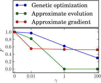
(a) One-qubit system with one-qubit ancilla. Target operation: NOT. The control is performed on the target qubit. Schematically shown in Figure 1a

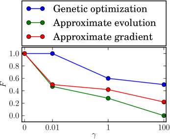
(b) Two-qubit system with no ancilla. Target operation: NOT. Schematically shown in Figure 1b

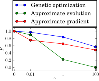
(c) One-qubit system with one-qubit ancilla. Target operation: NOT. The control is performed on the ancillary qubit. Schematically shown in Figure 1c

(d) Three-qubit system with no ancilla. Target operation: NOT. Schematically shown in Figure 1d

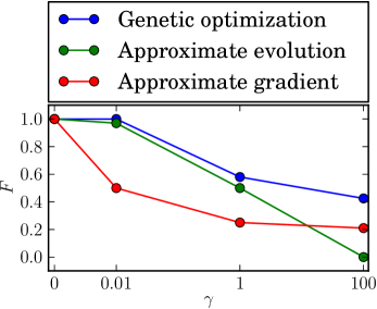
(e) Two-qubit system with one-qubit ancilla. Target operation: SWAP. The control is perfomed on the ancillary qubit. Schematically shown in Figure 1e

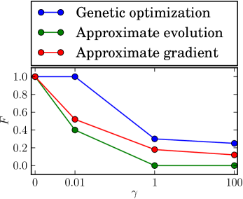
(f) Three-qubit system with no ancilla. Target operation: SWAP. Schematically shown in Figure 1f

Figure 2: Simulation results for the phase damping channel.

Next, in Figure 3 we show the results for the amplitude damping channel. Similarly to the phase damping case, the approximate evolution method performs the worst. The approximate gradient method gives far better results, especially for high values of $\gamma$. Again, this may be explained by the fact that in the approximate evolution, we have periods of coherent evolution, followed by decoherence. On the other hand, the genetic optimization performs quite well, even for high noise values we were able to find sets of control parameters which gave fidelity higher than a half. Again, the trade-off was the computation time. Genetic optimization took about an order of magnitude longer compared to other methods.

Unfortunately, all the studied methods appear to fail for $\gamma>0.01$ in the majority of investigated cases. For $\gamma=0.01$ only the genetic optimization gives a high value of fidelity.

The next step of our study focuses on comparing the algorithms when the computation times are on the same order of magnitude. To achieve this, we added more control pulses in the gradient based methods. In the case of both gradient based methods we used 128 pulses for the two-qubit scenario and 512 for the three-qubit scenario. The computation times are summarized in Table 3. Results are presented in Figures 4 and 5. Also in this setup the genetic optimization performs better compared to gradient based approaches. In this case the gap between these methods is narrower than in the case with equal number of control pulses.

	Genetic optimization		Approximate evolution		Approximate gradient
Number of qubits	2	3	2	3	2	3
Equal number of steps	810	30254	824	4147	781	3943
Equal computation time	8241	31029	8101	30846	8128	30447

Table 3: Average computation times in seconds for different simulation setups.

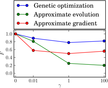
(a) One-qubit system with one-qubit ancilla. Target operation: NOT. The control is performed on the target qubit. Schematically shown in Figure 1a

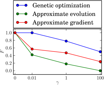
(b) Two-qubit system with no ancilla. Target operation: NOT. Schematically shown in Figure 1b

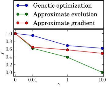
(c) One-qubit system with one-qubit ancilla. Target operation: NOT. The control is performed on the ancillary qubit. Schematically shown in Figure 1c

(d) Three-qubit system with no ancilla. Target operation: NOT. Schematically shown in Figure 1d

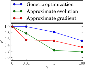
(e) Two-qubit system with one-qubit ancilla. Target operation: SWAP. The control is perfomed on the ancillary qubit. Schematically shown in Figure 1e

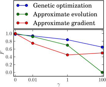
(f) Three-qubit system with no ancilla. Target operation: SWAP. Schematically shown in Figure 1a

Figure 3: Simulation results for the amplitude damping channel.

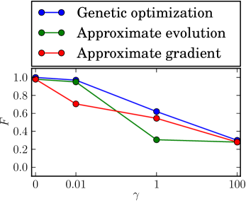
(a) One-qubit system with one-qubit ancilla. Target operation: NOT. The control is performed on the target qubit. Schematically shown in Figure 1a

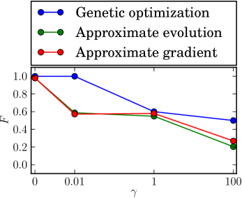
(b) Two-qubit system with no ancilla. Target operation: NOT. Schematically shown in Figure 1b

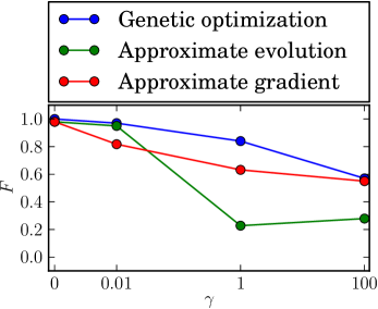
(c) One-qubit system with one-qubit ancilla. Target operation: NOT. The control is performed on the ancillary qubit. Schematically shown in Figure 1c

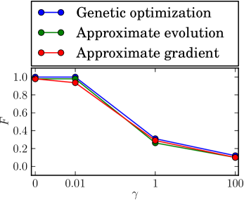
(d) Three-qubit system with no ancilla. Target operation: NOT. Schematically shown in Figure 1d

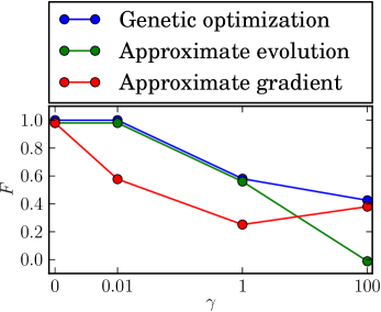
(e) Two-qubit system with one-qubit ancilla. Target operation: SWAP. The control is performed on the ancillary qubit. Schematically shown in Figure 1e

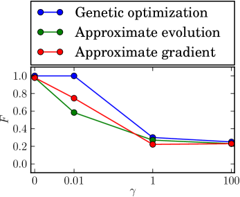
(f) Three-qubit system with no ancilla. Target operation: SWAP. Schematically shown in Figure 1f

Figure 4: Simulation results for the phase damping channel with equal computation time.

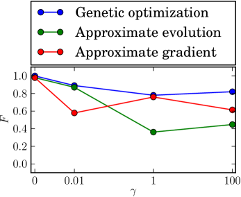
(a) One-qubit system with one-qubit ancilla. Target operation: NOT. The control is performed on the target qubit. Schematically shown in Figure 1a

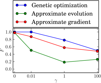
(b) Two-qubit system with no ancilla. Target operation: NOT. Schematically shown in Figure 1b

(c) One-qubit system with one-qubit ancilla. Target operation: NOT. The control is performed on the ancillary qubit. Schematically shown in Figure 1c

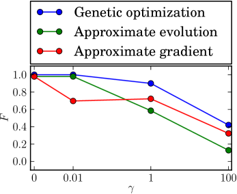
(d) Three-qubit system with no ancilla. Target operation: NOT. Schematically shown in Figure 1d

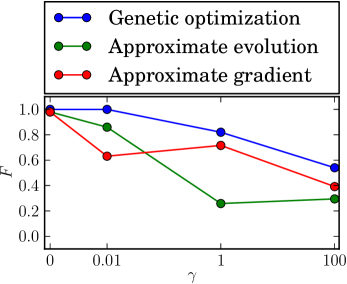
(e) Two-qubit system with one-qubit ancilla. Target operation: SWAP. The control is performed on the ancillary qubit. Schematically shown in Figure 1e

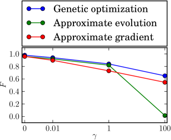
(f) Three-qubit system with no ancilla. Target operation: SWAP. Schematically shown in Figure 1a

Figure 5: Simulation results for the amplitude damping channel with equal computation time.

V Conclusions

We studied different methods of obtaining piecewise constant control pulses that implement an unitary evolution on a system governed by Kossakowski-Lindblad equation. The studied methods included genetic optimization and the BFGS algorithm with the use of fidelity gradient based on an approximate evolution of the quantum system and an approximate gradient method for the exact evolution case. Our results show that, by adding an ancilla, it is possible to implement a unitary evolution on a system under the Markovian approximation. Furthermore, the results heavily depend not only on the size, but also on the location of the ancilla in the spin chain.

What one can notice about the possibility to perform unitary computation in noisy quantum systems is that in majority of the cases it is much better to treat non-target qubits as an ancilla. When comparing systems extended with auxiliary qubits (labeled as $a,c,e$) and systems with no ancilla ($b,d,f$) the difference in possible approximation is emphatic.

The genetic optimization method outperforms gradient based methods in two studied setups: with equal number of control pulses and with equal computation time.

References

- Cheng et al. (2005) C.-J. Cheng, C.-C. Hwang, T.-L. Liao, and G.-L. Chou, Journal of Physics A: Mathematical and General 38, 929 (2005).
- Albertini and D’Alessandro (2002) F. Albertini and D. D’Alessandro, Linear Algebra and its Applications 350, 213 (2002), ISSN 0024-3795, URL http://www.sciencedirect.com/science/article/pii/S0024379502002902.
- Elliott (2009) D. Elliott, Bilinear control systems: matrices in action (Springer Verlag, 2009), ISBN 1402096127.
- d’Alessandro (2008) D. d’Alessandro, Introduction to quantum control and dynamics (Chapman & Hal, 2008).
- Burgarth and Giovannetti (2007) D. Burgarth and V. Giovannetti, Physical Review Letters 99, 100501 (2007), URL http://link.aps.org/doi/10.1103/PhysRevLett.99.100501.
- Burgarth et al. (2009) D. Burgarth, S. Bose, C. Bruder, and V. Giovannetti, Physical Review A 79, 60305 (2009), ISSN 1094-1622, URL http://link.aps.org/doi/10.1103/PhysRevA.79.060305.
- Puchała (2012) Z. Puchała, Quantum Information Processing (2012), URL http://dx.doi.org/10.1007/s11128-012-0391-x.
- Montangero et al. (2007) S. Montangero, T. Calarco, and R. Fazio, Physical Review Letters 99, 170501 (2007), URL http://link.aps.org/doi/10.1103/PhysRevLett.99.170501.
- Fisher et al. (2010) R. Fisher, F. Helmer, S. J. Glaser, F. Marquardt, and T. Schulte-Herbrüggen, Physical Review B 81, 085328 (2010), URL http://link.aps.org/doi/10.1103/PhysRevB.81.085328.
- Morzhin (2012) O. V. Morzhin, Automation and Remote Control 73, 1822 (2012).
- Dominy et al. (2013) J. M. Dominy, G. A. Paz-Silva, A. Rezakhani, and D. Lidar, Journal of Physics A: Mathematical and Theoretical 46, 075306 (2013).
- Qi (2013) B. Qi, Automatica 49, 834 (2013).
- Pawela and Puchała (2014) Ł. Pawela and Z. Puchała, Quantum Information Processing 13, 227 (2014), URL http://dx.doi.org/10.1007/s11128-013-0644-3.
- Pawela and Puchała (2013) Ł. Pawela and Z. Puchała, arXiv preprint arXiv:1306.6826 (2013).
- Li et al. (2009) J.-S. Li, J. Ruths, and D. Stefanatos, The Journal of chemical physics 131, 164110 (2009).
- Khodjasteh et al. (2010) K. Khodjasteh, D. A. Lidar, and L. Viola, Physical review letters 104, 090501 (2010).
- Schmidt et al. (2011) R. Schmidt, A. Negretti, J. Ankerhold, T. Calarco, and J. T. Stockburger, Physical review letters 107, 130404 (2011).
- Gawron et al. (2014) P. Gawron, D. Kurzyk, and Ł. Pawela, Quantum Information Processing 13, 665 (2014), URL http://dx.doi.org/10.1007/s11128-013-0681-y.
- Schulte-Herbrüggen et al. (2011) T. Schulte-Herbrüggen, A. Spörl, N. Khaneja, and S. Glaser, Journal of Physics B: Atomic, Molecular and Optical Physics 44, 154013 (2011).
- Hwang and Goan (2012) B. Hwang and H.-S. Goan, Physical Review A 85, 032321 (2012).
- Clausen et al. (2012) J. Clausen, G. Bensky, and G. Kurizki, Physical Review A 85, 052105 (2012).
- Floether et al. (2012) F. F. Floether, P. de Fouquieres, and S. G. Schirmer, New Journal of Physics 14, 073023 (2012).
- Heule et al. (2010) R. Heule, C. Bruder, D. Burgarth, and V. M. Stojanović, Physical Review A 82, 052333 (2010), URL http://link.aps.org/doi/10.1103/PhysRevA.82.052333.
- Nielsen and Chuang (2000) M. A. Nielsen and I. L. Chuang, Quantum Computation and Quantum Information (Cambridge University Press, 2000), ISBN 9780521635035.
- Zhu et al. (1997) C. Zhu, R. H. Byrd, P. Lu, and J. Nocedal, ACM Trans. Math. Softw. 23, 550 (1997), ISSN 0098-3500, URL http://doi.acm.org/10.1145/279232.279236.
- Byrd et al. (1995) R. H. Byrd, P. Lu, J. Nocedal, and C. Zhu, SIAM Journal on Scientific Computing 16, 1190 (1995), eprint http://epubs.siam.org/doi/pdf/10.1137/0916069, URL http://epubs.siam.org/doi/abs/10.1137/0916069.
- Havel (2003) T. F. Havel, Journal of Mathematical Physics 44, 534 (2003).
- Machnes et al. (2011) S. Machnes, U. Sander, S. J. Glaser, P. de Fouquières, A. Gruslys, S. Schirmer, and T. Schulte-Herbrüggen, Physical Review A 84, 022305 (2011), URL http://link.aps.org/doi/10.1103/PhysRevA.84.022305.
- Spector (2004) L. Spector, Automatic quantum computer programming: a genetic programming approach (Springer, 2004).
- Gepp and Stocks (2009) A. Gepp and P. Stocks, Genetic Programming and Evolvable Machines 10 (2009), URL http://dx.doi.org/10.1007/s10710-009-9080-7.
- Goldberg (1989) D. Goldberg, Genetic Algorithms in Search, Optimization, and Machine Learning (Addison-Wesley Professional, 1989).
- Sadowski (2013) P. Sadowski, International Journal of Quantum Information 11, 1350067 (2013), URL http://dx.doi.org/10.1142/S0219749913500676.