An ab initio study of magneto-electric coupling of $\rm YMnO_{3}$

Abstract

The present paper proposes the direct calculation of the microscopic contributions to the magneto-electric coupling, using ab initio methods. The electrostrictive and the Dzyaloshinskii-Moriya contributions were evaluated individually. For this purpose a specific method was designed, combining DFT calculations and embedded fragments, explicitely correlated, quantum chemical calculations. This method allowed us to calculate the evolution of the magnetic couplings as a function of an applied electric field. We found that in $\rm YMnO_{3}$ the Dzyaloshinskii-Moriya contribution to the magneto-electric effect is three orders of magnitude weaker than the electrostrictive contribution. Strictive effects are thus dominant in the magnetic exchange evolution under an applied electric field, and by extension on the magneto-electric effect. These effects remain however quite small and the modifications of the magnetic excitations under an applied electric field will be difficult to observe experimentally. Another important conclusion is that the amplitude of the magneto-electric effect is very small. Indeed, it can be shown that the linear magneto-electric tensor is null due to the inter-layer symmetry operations.

I Introduction

Multiferroic materials have been known since the work of Pierre Curie in 1894 PCurie , and of E. Bauer in 1926 Bauer . During the last years they regained an increased attention due to the discovery of colossal magneto-electric effects ME_regain . In such systems, the magnetic properties (magnetization, magnetic ground state, etc.) can be controlled using an electric field, and the electric properties (polarization, dielectric constant, etc.) can be controlled using a magnetic field. In spite of the multiple studies done over the years, the microscopic origin of the magneto-electric coupling is still ill-known. While the spin-orbit coupling is the only term in the Hamiltonian that couples the magnetic degrees of freedom with the charge degrees of freedom, others effects such as electrostrictive / magnetostrictive indirect coupling have also been proposed as candidates for the origin of the magneto-electric coupling. The aim of this paper will thus be to directly compute the different microscopic mechanisms contributing to the magneto-electric effect.

Multiferroic systems are generally classified into type I and type II compounds. Type I materials are characterized by a paraelectric / ferroelectric transition distinct from the magnetic transition, while for type II systems ferroelectricity appears at a magnetic transition. In this paper, we will focus on one of the most typical type I materials, $\rm YMnO_{3}$. This compound exhibits a paraelectric /  ferroelectric transition at high temperature (with the appearance of a spontaneous polarization along the c axis), and an antiferromagnetic transition at 74 K. A magneto-electric coupling in the low temperature phase has been evidenced by several groups ME_YMO through the apparition of an anomaly in the dielectric constant at the Néel temperature. This magneto-electric coupling was first explained by Goltsev et al. Goltsev as a piezomagnetic interaction between ferroelectric and antiferromagnetic domain walls. Then Hanamura et al. Hanamura proposed a spin-orbit origin, through a dependence of the exchange integrals to the polarization sign. Finally, Lee et al. Park08 proposed an electrostrictive / magnetostrictive microscopic origin. $\rm YMnO_{3}$ thus looks as a good candidate for a theoretical investigation of the origin of the magneto-electric coupling. In addition, it presents the advantage to display only one magnetic species, the manganese ions.

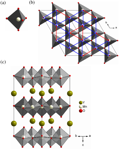
Figure 1: (Color online) Structure of the $\rm YMnO_{3}$ compound. (a) $\rm MnO_{5}$ bipyramid, (b) two-dimensional triangular layers of $\rm MnO_{5}$ bipyramids, the two types of Mn-Mn bonds are respectively underlined in blue and red, (c) complete crystal structure.

$\rm YMnO_{3}$ crystallizes in an hexagonal structure, in the $\rm P6_{3}cm$ space group under the paraelectric / ferroelectric transition. The structure is based on corner-sharing $\rm MnO_{5}$ bipyramids, organized in two-dimensional triangular layers (see figure 1). The yttrium atoms are located in between the bipyramids layers. The triangular arrangement of the manganese atoms is not ideal and there are two different Mn-Mn type of bonds (see figure 1b). Structurally, the antiferromagnetic transition is seen as an isostructural $\rm P6_{3}cm$ to $\rm P6_{3}cm$ one. This transition is however associated with large atomic displacements Park08 , strongly affecting the polarization amplitude Park05 ; YMO1 . The associated magnetic order was long believed to belong to the totally symmetric irreducible representation of the $\rm P6_{3}cm$ magnetic group GpeMag , however it was recently shown that the magnetic group can only be $\rm P6^{\prime}_{3}$, loosing the symmetry planes orthogonal to the layers Tapan ; YMO1 .

The magnetism is due to $\rm Mn^{3+}$ manganese ions ($3d^{4}$) in a high spin state (S=2). The trigonal symmetry of the bipyramids splits the $3d$ orbitals as pictured in figure 2, leaving an empty $3d_{z^{2}}$ orbital. The resulting atomic spins form a triangular lattice with frustrated antiferromagnetic interactions. Neutron scattering experiments show in plane orientation of the manganese spins with a 120^∘ arrangement GpeMag . However, more recently, a very weak ferromagnetic component, oriented along the c axis, has been observed and shown to be due to the spin-orbit coupling YMO1 . At this point let us note that the spin-orbit interaction (as well as the Dzyaloshinskii-Moriya effective model) breaks the $\rm P6_{3}cm$ symmetry group and induces a lowering of the symmetry to the $\rm P6^{\prime}_{3}$ magnetic group and associated $P6_{3}$ crystallographic group.

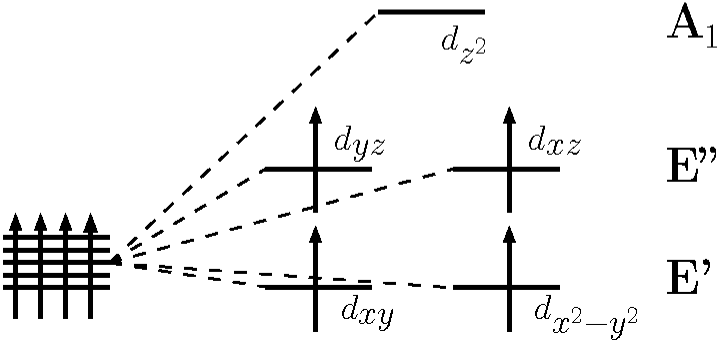
Figure 2: Splitting of the $3d$ orbitals for the $\rm Mn^{3+}$ ions.

The present paper will be organized as follow. The next section will be devoted to the presentation of the method used for the calculation of the magneto-electric coupling. Section III will present the results on the exchange integrals while section IV will present the results on the magneto-electric coupling. Finally, the last section will propose a conclusion.

II Computing the microscopic contributions to the magneto-electric effect

How to compute the microscopic contributions to the magneto-electric effect ? One possibility would be to compute the electric properties (polarization, dielectric constant, etc.) as a function of an applied magnetic field. This is the line followed by some authors, applying a Zeeman field within a density functional calculation P_H . Another possibility is to compute the magnetic state as a function of an applied electric field. In this work, we chose to use the second method. Indeed, the polarization or dielectric constant can only be computed using density functional theory (DFT) or related mean-field methods (see for instance reference mostovoy, ). However, such methods encounter difficulties to accurately evaluate the magnetic couplings, crucial for the magneto-electric effect. For instance, in the present system, even when using the hybrid B3LYP functional, DFT calculations of the exchange integral yield -0.59 meV SASS , to be compared with the -2.3meV J_Petit and -3 meV J_Park evaluations from inelastic neutrons scattering and to the -2.7meV SASS evaluation found using the fully correlated wave-function SAS+S method such as in the present work (see below for details). We will thus compute, using the SAS+S ab initio method (with and without spin-orbit interactions) the magnetic coupling constants as a function of an applied electric field. These integrals can in a second step be used within the underlying effective magnetic Hamiltonian : the Heisenberg model, corrected by the Dzyaloshinskii-Moriya interaction DzMy , on a two dimensional triangular lattice.

$$H=-\sum_{<i,j>}J_{ij}\,\vec{S}_{i}\cdot\vec{S}_{j}+\vec{D}_{ij}\cdot\vec{S}_{i}\wedge\vec{S}_{j}$$ (1)

where the sum over $<i,j>$ runs over all Mn-Mn nearest neighbor bonds. The ab-initio parameterized model can then be used to derive the magneto-electric coupling tensor.

The next question is now :  “what is the main effect of an applied electric field ?”. According to J. Iñiguez Jorge , the main effect is the nuclear displacements induced by the electric field. Indeed, most of the time, the external field is efficiently screened and the orbital polarization due to the applied field can be neglected P_H ; Jorge . Since an electric field does not directly couple to spins, the spin contribution (important when a magnetic field is applied) only comes through the spin-orbit term. When the spin-orbit coupling and orbital moment remain small (as in the present system, see below) so will be the orbital polarization. Of course this would not be the case in systems where the spin-orbit is rather large polso . The atomic displacements $\vec{d}$ can be determined using the Newton’s second law as

$$\overline{\vphantom{\rule{1.0pt}{5.54861pt}}\smash{\overline{Z}}}^{\,\star}\cdot\vec{E}\,=\,\overline{\vphantom{\rule{1.0pt}{5.54861pt}}\smash{\overline{\mathcal{H}}}}\cdot\vec{d}\qquad\Leftrightarrow\qquad\vec{d}\,=\,\overline{\vphantom{\rule{1.0pt}{5.54861pt}}\smash{\overline{\mathcal{H}}}}^{-1}\cdot\overline{\vphantom{\rule{1.0pt}{5.54861pt}}\smash{\overline{Z}}}^{\,\star}\cdot\vec{E}$$ (2)

where $\vec{E}$ is the applied electric field, $\overline{\vphantom{\rule{1.0pt}{5.54861pt}}\smash{\overline{Z}}}^{\,\star}$ is the Born charge tensor, $\overline{\vphantom{\rule{1.0pt}{5.54861pt}}\smash{\overline{\mathcal{H}}}}$ is the Hessian matrix of the electronic Hamiltonian and $\vec{d}$ is the sought displacements vector.

Our aim is to compute the magnetic exchange integrals under such displacements. However, there is no theoretical technique able to simultaneously give, with reliable accuracy, the elastic effects and the magnetic integrals. Indeed, while the former are induced by the system as a whole (infinite and total electronic density) and little depend on the Fermi electrons (they account for only a small part of the total energy), the latter are essentially local and dominated by the physics of the Fermi level strongly correlated electrons. An accurate evaluation of the magnetic integrals requires a thorough treatment of the electron correlation. We thus developed a two-steps approach, combining density functional (DFT) calculations for the elastic part and quantum chemical embedded fragments calculations for the magnetic part. The first step consists in the calculation of the Hessian matrix and the Born effective charge tensor using DFT. The atomic displacements induced by an applied electric field are then evaluated using equation 2. The second step consists in computing the magnetic exchange integrals associated with the new geometries. For this purpose, we used the SAS+S method SASS that was specifically designed for the accurate evaluation of magnetic excitations, in strongly correlated systems with numerous open shells per atom. The SAS+S method is a configurations interaction method (exact diagonalization within a selected configurations space) explicitly including the correlation within the metals $d$ shells, the ligand-to-metal charge transfers, and the screening effects on both phenomena. It allows an accurate calculation of low energy excitation spectra as magnetic excitations. This method can however only be applied on finite systems. Appropriate embedded fragments were thus designed. In the present work the fragments were built from two Mn ions and their first coordination shells for the quantum part (see figure 3). Indeed, it has been shown by different groups loc that the magnetic exchanges are local (the only important non local effect is the Madelung potential that, in the present work, was taken into account through the embedding , see below) and that the enlargement of the fragment, further than the first coordination shell of the magnetic atoms, does not modify in any significant manner the evaluation of the effective magnetic exchanges.

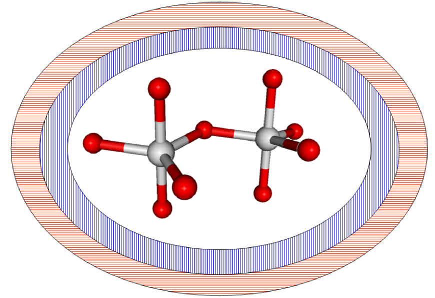
Figure 3: (Color online) Schematic representation of the embedded clusters. The quantum part is explicitely shown, the vertically dashed (blue) surrounding part represents the Total Ion Pseudopotentials (two shells of neighboring atoms), while horizontally dashed (red) part represents the punctual charges ($\sim$ 66000 renormalized point charges).

These quantum fragments were embedded in an environment reproducing on them the main effect of the rest of the crystal ; (i) the exclusion effects of the surrounding electrons and (ii) the long range Madelung potential. The former were modeled using total ion pseudopotentials TIP at surrounding atomic positions. The latter was computed using a set of punctual charges, located at atomic positions. These charges were renormalized on the external part, following the scheme described in reference Alain_env, , so that to ensure an exponential converge of the Madelung potential.

In order to differentiate the relative importance of the different mechanisms responsible for the magneto-electric coupling, we computed the embedded clusters magnetic spectrum, as a function of an applied electric field, with and without the spin-orbit interaction.

Technical details

The DFT calculations were performed using the CRYSTAL09 package CRYSTAL09 . Since the manganese 3d shells are strongly correlated we used the hybrid B1PW B1PW functional (hybrid functional specifically derived for the treatment of ferroelectric compounds) in order to better take into account the self-interaction cancellation. Small core pseudo-potentials were used for the heavy atoms (Mn and Y) associated with semi-valence and valence $2\zeta$ and $2\zeta$ plus polarization basis sets Bases1 . The oxygen ions were represented in an all-electrons basis set of $2\zeta$ quality specifically optimized for $\rm O^{2-}$ ions Bases1 . This method was used with great success in a previous work to compute the phonon spectrum, which agreement with experimental observations guarantees its quality. For the details, see reference YMO2, . The SAS+S method was performed using successively the MOLCAS MOLCAS package for the integrals and the fragment orbitals calculations, the CASDI package for the configurations interaction, and the EPCISO EPCISO package for the spin-orbit calculations. 3-$\zeta$ valence basis and core pseudopotentials set were used in the calculation Bases2 .

III Results : the exchange integrals in the $\rm YMnO_{3}$ compound

The magnetic exchange integrals are computed from the excitation energies between the $S=4$ and $S=3$ states of the embedded fragments. Indeed in a Heisenberg picture, the excitation energy between those states is associated with $4J$.

In the $\rm YMnO_{3}$ compound, there are two independent magnetic integrals, associated with the two previously mentioned Mn-Mn types of bond (see figure 1b). We computed the magnetic integrals associated with the short Mn-Mn bonds $J_{s}=-2.73$ meV, and the long Mn-Mn bonds $J_{l}=-2.47$ meV. These values compare well with the evaluations obtained from the fitting of inelastic neutron scattering on a homogeneous triangular model : $J=-2.3$ meV J_Petit and $J=-3$ meV J_Park , thus validating the quality of the SAS+S method.

IV Results : the magneto-electric coupling

The application of an electric field in the $(\bf{a},\bf{b})$ plane destroys the punctual symmetries and increases the number of non-equivalent magnetic integrals from two to nine (see figure 4).

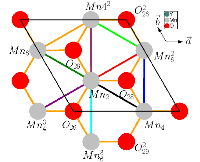
Figure 4: (Color online) Representation of the nine magnetic interactions induced by the application of an electric field in the $(\bf{a},\bf{b})$ plane.

IV.1 Without the spin-orbit interaction

We first focused on one of the $\rm Mn-Mn$ bonds, and studied the evolution of its magnetic coupling as a function of an applied electric field in the three crystallographic directions. The bond under consideration is the short bond referred as $\rm Mn_{2}-O_{28}-Mn^{2}_{6}$ and pictured in red on figure 4 — Mn atoms are located at (x_Mn,x_Mn,z_Mn+1/2) and at (1,1-x_Mn,z_Mn+1/2). The results are displayed on figure 5.

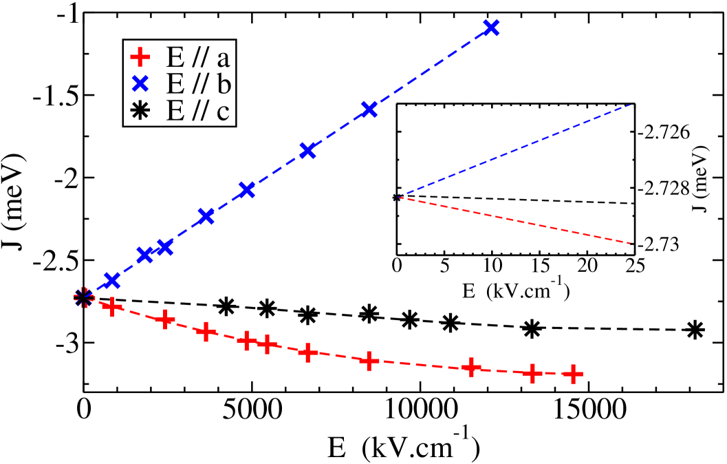
Figure 5: (Color online) Evolution of the exchange integral ($\rm Mn_{2}-O_{28}-Mn^{2}_{6}$ dimer) as a function of an applied electric field along the $\bf a$, $\bf b$ and $\bf c$ directions. The inset details the part of the curves associated with experimentally accessible electric fields.

When the electric field is applied along the ${\bf c}$ direction, the magnetic coupling remains essentially unchanged. When the electric field is applied along the ${\bf b}$ direction, that is perpendicular to the $\rm Mn-Mn$ bond axis, the exchange integral is strongly affected by the field and its antiferromagnetic character is reduced. Its behavior is essentially linear as a function of the electric field $E$ with $J=-2.73+1.36\times 10^{-4}\,E$. When the field is along the ${\bf a}$ direction, the $\rm Mn-Mn$ bond presents an angle of 30^∘ with the field direction. In this case the antiferromagnetic character of the exchange integral is slightly increased.

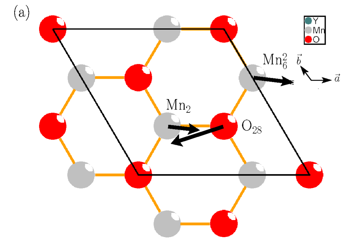
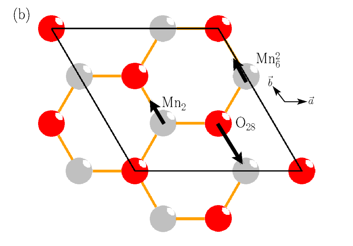
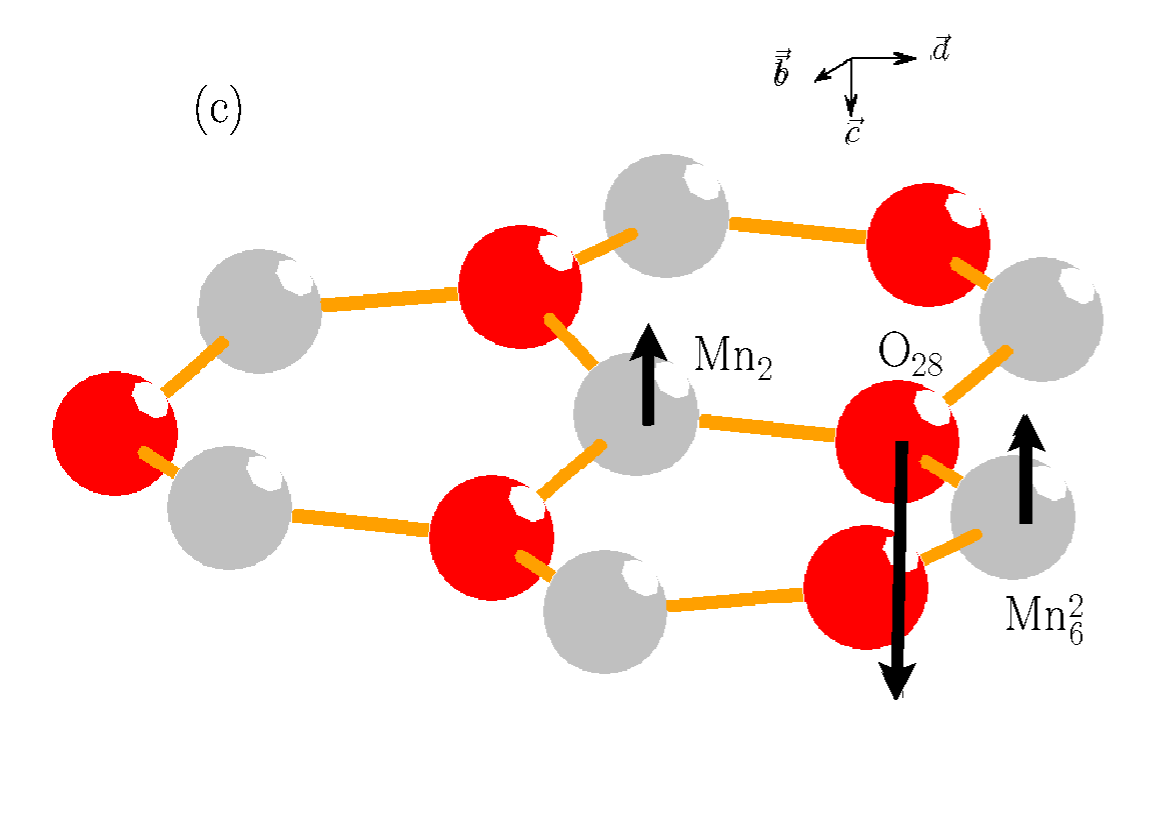
Figure 6: (Color online) Atomic displacements for an applied electric field along the (a) ${\bf a}$ direction, (b) ${\bf b}$ direction and (c) ${\bf c}$ direction. For experimentally accessible fields the displacements are negligible. For instance an applied field of 10 kV/cm along the a direction one gets $\delta d_{\rm Mn-Mn}=-1\times 10^{-9}\rm\AA$, $\delta d_{\rm Mn-O}=-1.7\times 10^{-6}\text{ and }0.7\times 10^{-6}\rm\AA$, $\delta\widehat{\rm Mn-O-Mn}=5\times 10^{-5}$. For an applied field of $\sim 50kV/cm$ one gets along the a direction : $\delta d_{\rm Mn-Mn}=7\times 10^{-4}\rm\AA$, $\delta d_{\rm Mn-O}=-6\times 10^{-2}\text{ and }3\times 10^{-2}\rm\AA$, $\delta\widehat{\rm Mn-O-Mn}=1.3^{\circ}$ ; along the b direction : $\delta d_{\rm Mn-Mn}=3\times 10^{-4}\rm\AA$, $\delta d_{\rm Mn-O}=3\times 10^{-2}\rm\AA$, $\delta\widehat{\rm Mn-O-Mn}=-2.6^{\circ}$ ; and along the c direction : $\delta d_{\rm Mn-Mn}=-2\times 10^{-3}\rm\AA$, $\delta d_{\rm Mn-O}=-4\times 10^{-3}\rm\AA$, $\delta\widehat{\rm Mn-O-Mn}=0.3^{\circ}$.

Figure 6 pictures the atomic displacements when the field is applied along the three directions. The $J$ behavior as a function of the electric field direction can be understood considering these induced displacements on direct and super-exchange terms. When the field is along the ${\bf c}$ direction the Mn and O planes are closing in, increasing the antiferromagnetic character. This increase remains very small since the Mn and O planes are already very close ($\sim 0.2\,\rm\AA{}$) and the super-exchange terms varies as $1-\alpha h^{2}$ where $h$ is the inter-plane distance. Second, the $\rm Mn-O-Mn$ angle is slightly opening up, decreasing the antiferromagnetic character. As a result, the electric field has little effect. When the field is along the ${\bf b}$ direction, the main effect is to increase the Mn-O bond lengths, and thus to reduce the magnetic-to-ligand orbitals overlap, responsible for the super-exchange mechanism. As a result, the antiferromagnetic character is strongly reduced. Finally, when the field is applied along the ${\bf a}$ direction, one of the Mn-O distance is reduced, while the other one is increased, the Mn-Mn distance remaining unchanged. This mechanism results in an opening of the $\rm Mn-O-Mn$ angle. While the effects of the distance changes compensate each other, the Mn-O-Mn angle opening increases the metal-to-ligand orbitals overlap, thus increasing the superexchange antiferromagnetic contribution. Let us now concentrate on electric field values experimentally accessible (see inset of figure 5), one should notice that even for fields as large as $10\rm kV.cm^{-1}$, the renormalization of the magnetic coupling remains very small, at most of the order $10^{-3}$ meV. One should thus unfortunately conclude that the effect of an electric field on the $\rm YMnO_{3}$ magnetic spectrum should be experimentally difficult to observe.

Due to the hexagonal symmetry of $\rm YMnO_{3}$, applying the field along the ${\bf a}$ or ${\bf b}$ directions is equivalent by symmetry on the whole system. We will thus compute the nine different exchange integrals with the field applied along the ${\bf a}$ direction. Figure 7 displays the results for the nine dimers.

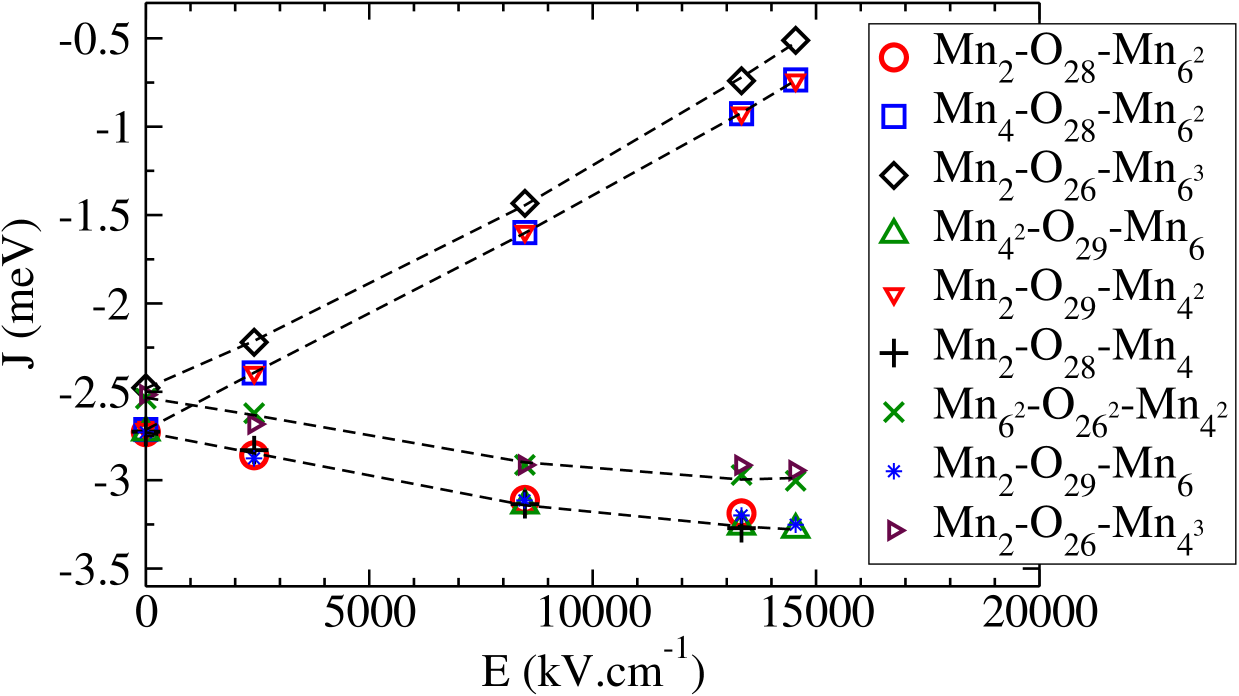
Figure 7: (Color online) Evolution of the nine different magnetic couplings under an applied electric field along the $\bf a$ direction.

One sees that there are only two behaviors, corresponding to the field perpendicular to the Mn-Mn bonds, and to the field at 30^∘ degrees with the Mn-Mn bonds. For each behavior, the two sets of curves are associated with the two types of Mn-Mn bonds in zero field.

IV.2 With the spin-orbit interaction

We then computed the spin orbit correction on the embedded fragments magnetic spectrum, using the ab initio wave-function Epciso code from the Lille’s group EPCISO . As implicitly done in the previous section (where the ab-initio results were mapped into an effective Heisenberg model) we will map the ab-initio spin-orbit correction onto an effective Dzyaloshinskii-Moriya model ($\vec{D}\cdot(\vec{S}_{i}\wedge\vec{S}_{j})$). Following the calculation done by Moriya on a single electron system DzMy , one can show that the ground state corrections due to the spin orbit coupling for our four electrons per site system, can also be mapped onto a Dzyaloshinskii-Moriya model. The latter yields

$$\hat{H}_{\text{DM}}\,\Psi_{\text{GS}} = (D_{y}+iD_{x})\,\Psi_{S=1,S_{z}=1}$$

$$\;-\;(D_{y}-iD_{x})\,\Psi_{S=1,S_{z}=-1}\;-\;iD_{c}\,\sqrt{2}\,\Psi_{S=1,S_{z}=0}$$

where $D_{x}$ and $D_{y}$ correspond to the in-plane components of the Dzyaloshinskii-Moriya prefactor and $D_{c}$ to its out of plane component. At this point let us note that, assuming purely atomic magnetic orbitals, and second order perturbation in the spin-orbit operator, the component on $\Psi_{S=1,S_{z}=0}$ should be zero, and thus so should be $D_{c}$. Similarly, under this hypothesis $D_{x}=D_{y}=D_{ab}$. The $D_{ab}$ and $D_{c}$ amplitudes can be extracted from ab-initio calculations as the spin-orbit Hamiltonian matrix terms expressed on the ab-initio spin-only states. Results for a few representative points are displayed in table 1.

Field direction	Field amplitude	$D_{ab}$	$D_{c}$
	(kV.cm-1)	(meV)	(meV)
-	0	0.00058	0.00383
a	36359	0.00069	0.00465
a	145436	0.00121	0.00841
a	181795	0.00151	0.01001
b	48479	0.00037	0.00193
b	181795	0.00169	0.00328
c	84838	0.00053	0.00403
c	109077	0.00054	0.00414

Table 1: Dzyaloshinskii-Moriya vector $\vec{D}$ as a function of an applied electric field. $\vec{D}$ was extracted from ab-initio wave function calculations for a few representative values of the field amplitude.

One see immediately that the Dzyaloshinskii-Moriya interaction remains extremely small in this system with an order of magnitude $10^{2}$ to $10^{3}$ weaker than the exchange part. Its modulation as a function of the field is only of a few $10^{-3}$ meV.

The exchange-striction contributions are thus much larger than the spin-orbit ones. These direct, quantitative calculations confirm the conclusions found by indirect methods such as (i) the fact that DFT evaluation of the spontaneous polarization is essentially independent of the magnetic state YMO2 , or (ii) the giant magneto-elastic coupling found by Lee et al. Park08 .

V The magneto-electric coupling tensor

From the above calculations one should be able to extract the linear magneto-electric tensor : $\alpha$. Indeed, in the magnetic phase, as soon as one is a little away from the transition temperature, the free energy is dominated by the magnetic energy and one can safely assume that

$$\alpha = -\left.\frac{\partial^{2}{\cal F}}{\partial\vec{\cal E}\,\partial\vec{\cal H}}\right|_{{{\cal E}=\vec{0}\atop{\cal H}=\vec{0}}}\;=\;\sum_{\vec{R}}\sum_{<i,j>}\frac{\partial^{2}J_{ij}\langle\vec{S}_{i}\cdot\vec{S}_{j}\rangle}{\partial\vec{\cal E}\,\partial\vec{\cal H}}$$

$$\simeq \sum_{\vec{R}}\sum_{<i,j>}\frac{\partial J_{i,j}}{\partial\vec{\cal E}}\cdot\left(\frac{\partial\langle\vec{S}_{i}\rangle}{\partial\vec{\cal H}}\cdot\langle\vec{S}_{j}\rangle\,+\,\langle\vec{S}_{i}\rangle\cdot\frac{\partial\langle\vec{S}_{i}\rangle}{\partial\vec{\cal H}}\right)$$

The present ab-initio calculations gave us the $\frac{\partial J_{i,j}}{\partial\vec{\cal E}}$ factors. For the $\frac{\partial\langle\vec{S}_{i}\rangle}{\partial\vec{\cal H}}$ one, the $\rm Mn^{3+}$ ions being $S=2$ they can be treated as classical spins and the solution of the Heisenberg Hamiltonian under a magnetic field derived for the 2D triangular lattice associated with each layer. Labeling each of the three sublattices $\lambda$, $\mu$, $\nu$ one gets for the $z=0$ layer

$$\alpha_{z=0} = \frac{\mu_{0}\mu_{B}\,S}{3J}\;$$

$$\left\{\frac{\partial J_{\lambda,\mu}}{\partial\vec{\cal E}}\otimes\left(\begin{array}[c]{c}\frac{3\sqrt{3}}{2}\\ \frac{3}{2}\\ 0\end{array}\right)\,+\,\frac{\partial J_{\mu,\nu}}{\partial\vec{\cal E}}\left(\begin{array}[c]{c}0\\ -3\\ 0\end{array}\right)\,+\,\frac{\partial J_{\nu,\lambda}}{\partial\vec{\cal E}}\left(\begin{array}[c]{c}\frac{\sqrt{3}}{2}\\ \frac{3}{2}\\ 0\end{array}\right)\right\}$$

where $S$ is the norm of the atomic spins. Applying now the symmetry operations relating the $z=0$ and the $z=1/2$ layers, one gets $\frac{\partial J_{i,j}(z=0)}{\partial\vec{\cal E}}=-\frac{\partial J_{i,j}(z=1/2)}{\partial\vec{\cal E}}$ and thus

$$\alpha=\left(\begin{array}[c]{ccc}0&0&0\\ 0&0&0\\ 0&0&0\end{array}\right)$$

This conclusion should be put in perspective with experimental data. Indeed, the measurement of the dielectric constant as a function of the temperature does not exhibit any divergence YMO1 as should be the case, according to Landau analysis, for a linear magneto-electric coupling ; that is $\alpha$ must be null as we found from symmetry analysis.

VI Conclusion

We computed, using a combination of different first principle methods, the evolution of the magnetic exchange integrals as a function of an applied electric field. For this purpose a specific procedure was designed, combining DFT calculations for the degrees of freedom related to the whole electronic density (polarization, Born charge tensor, Hessian matrix), and embedded fragments, explicitely correlated, quantum chemical calculations for the degrees of freedom related to the strongly correlated Fermi electrons (magnetic couplings). One should notice that this method was able to reach experimental accuracy on the magnetic couplings without any adjustable parameter.

Our calculations allowed us to investigate the relative importance of the exchange-striction and of the spin-orbit effects. We found that, in this system, the Dzyaloshinskii-Moriya contribution to the magneto-electric effect remains about two orders of magnitude weaker than the exchange-strictive contribution. These results support previous hypotheses proposed from the observation of a giant magneto-elastic effect Park08 , and from the insensitivity of DFT polarization calculations to the magnetic ordering YMO2 . Another important conclusion for the experimentalists comes from the weakness of the magnetic exchanges variation, under applied electric field of experimentally accessible amplitude.

Finally, knowing the dependence of the exchange integrals as a function of an applied electric field, one can compute the linear magneto-electric coupling tensor. Our calculations however showed that this tensor is null, due to the symmetry operations relating the two magnetic layers belonging to the unit cell along the c direction.

$\rm YMnO_{3}$ is a type I multiferroic compound, that is the magnetic and ferroelectric transitions are not directly coupled. For type II multiferroic systems this is not the case, and the spin-orbit interaction is usually assumed to be responsible for the magneto-electric coupling typeII . It would thus be of great interest to perform such calculations for a type II compound in order to clarify the role and relative importance of the magnetostrictive - electrostrictive and spin-orbit interactions.