CCNY-HEP-13/6

October 2013

Quantum field theories with boundaries and novel instabilities
 
 
T.R. Govindarajan^a and V.P. Nair<sup>b

a</sup> Chennai Mathematical Institute
Siruseri, TN 603103
India
^bPhysics Department
City College of the CUNY
New York, NY 10031
E-mail: ^a trg@cmi.ac.in ^b vpn@sci.ccny.cuny.edu

Abstract

Quantum physics on manifolds with boundary brings novel aspects due to boundary conditions. One important feature is the appearance of localised negative eigenmodes for the Laplacian on the boundary. These can potentially lead to instabilities. We consider quantum field theories on such manifolds and interpret these as leading to the onset of phase transitions.

1 Introduction

In this paper, we consider the problem of general boundary conditions for quantum fields defined on a manifold with a boundary. Such manifolds are not only of mathematical interest, but physically required in several condensed matter systems as well as semiclassical gravity and string theory. For simplicity, one might even start by considering a free scalar field $\phi$ with a kinetic term which is given by the Laplacian acting on $\phi$. The choice of boundary conditions must be consistent with the self-adjointness requirements on the Laplacian and hence are generally described by the von Neumann theory of self-adjoint extensions [1]. This theory has recently been elegantly rephrased in [2] and has naturally led to a framework for analyzing the effects of boundary conditions which are more general than Neumann, Dirichlet. Berry used general Robin boundary conditions to explain novel behaviour of the spectrum [3]. One of us used Robin boundary conditions to obtain novel bound states localised on the boundary to understand blackhole entropy[4]. These boundary conditions have effects on the Casimir energy and this has been exhaustively analysed in [5, 6]. There are a number of related variants which have also been studied before. Partially transparent boundaries for scalar fields [7] and for the electromagnetic case [8] have been investigated. The case when boundary conditions (which can also lead to instabilities as explained below) can be modeled via $\delta$-functions have also been considered [9].

The set of boundary conditions is given by the choice of a unitary operator $U$, or by the hermitian operator ${\cal K}$ which is its Cayley transform, on the boundary values of the fields viewed as elements of a Hilbert space of $L^{2}$-functions on the boundary. (We emphasize that one could have more general boundary values for fields which are not square-integrable, singular charge distributions on the boundary being one class of such examples.We will only consider cases which are $L^{2}$-functions.) Specifically, the most general boundary conditions are given by

$$\phi+i\partial_{n}\phi = U\,(\phi-i\partial_{n}\phi)$$

$$(\phi+i\partial_{n}\phi)(x) = \oint_{y}U(x,y)\,(\phi-i\partial_{n}\phi)(y)$$ (1)

where $\partial_{n}\phi$ denotes the normal derivative of the field. The alternate way to write this in terms of the Cayley transform ${\cal K}$ is

$$\partial_{n}\phi=-i\left({U-1\over U+1}\right)\,\phi\equiv-{\cal K}\,\phi$$ (2)

The simplest choices, ${\cal K}=0$ and ${\cal K}\rightarrow\infty$, correspond to Neumann and Dirichlet conditions, respectively. These are special points in the space of boundary conditions. The choice of ${\cal K}$ being proportional to the identity operator on the Hilbert space of boundary values is the the Robin condition. One could choose more general ones with different eigenvalues for ${\cal K}$ for different modes on the boundary. The important point is that there are an infinity of choices for ${\cal K}$ which leads to negative eigenvalues for Laplacian associated with eigenmodes which are localised close to the boundary. Such novel states have been exploited earlier in several areas, like quantum hall effect, topological insulators and blackhole physics [10]. Clearly such modes will also be important for the Casimir effect and related issues such as the pair production of particles. A point worth emphasizing is that these modes of negative eigenvalues can occur infinitesimally close (in the space of boundary conditions) to the “good choices” like Dirichlet or Neumann. Generically, all such choices lead to instabilities in many body physics. Our experience in physics is that whenever instabilities arise, there is a way out, usually via a phase transition or change of ground state. The classic example is, of course, spontaneous symmetry breaking where a negative (mass)² term signals the phase transition to a new stable choice of ground state. The purpose of the present paper is to ask to what extent a similar scenario can work out for instabilities due to the boundary condition.

In most field-theoretic calculations, normally, the starting point is to consider the theory at zero temperature. This means that unless excitations are introduced via external sources, the state of interest is the ground state. If needed, this can then be upgraded to finite temperature with all states contributing, each weighted with the corresponding Boltzmann factor. But in the present case, where the notion of a ground state for the field theory is not clear, our basic strategy will be to consider the partition function at finite temperature and then ask whether it is possible to lower the temperature to zero. We may view the partition function as given by the functional integration over the fields in Euclidean spacetime with periodicity along the imaginary-time direction. We will then consider conditions under which the Euclidean functional integral is well-defined. By considering the limit of this case where the instabilities will begin to appear, we can get an understanding of how the transition, if nay, should manifest itself.

In Sec.2, we will briefly consider a couple of examples of how the negative eigenvalues arise. This is meant primarily to set the framework. In Sec.3, we will present Bose-Einstein condensation in terms of the Euclidean functional integral at finite temperature and see that a similar condensation is possible in the case of manifolds with boundary due to the presence of negative eigenvalues for $-\nabla^{2}$. A key issue here is the existence of a conserved charge (or particle number) with a corresponding chemical potential. Since the particle number is fixed, an infinite occupation number for the states of negative energy is not possible and the theory has a many-body ground state.

In the following section (Sec.4), we consider a real massless scalar field. Since there is no conserved quantum number in this case, the situation is different. We show how a Euclidean functional can be defined if we impose a set of restrictions on the theory. Effectively, at the level of free particles, there is always a finite temperature, which will play the role that the absolute zero of temperature does in normal theories with no negative eigenvalues for the Laplacian. There should also be an “unattainability rule” for this value of temperature, just as the third law of thermodynamics dictates for normal systems.

Once interactions are introduced, the story can change. We show in Sec.5 how corrections can be calculated in the theory. The modes with negative eigenvalues lead to a potential which is repulsive near the boundary and can alter the eigenstates and eigenvalues. This gives a way of removing singularities in the Euclidean functional integral. Finally we end up with a discussion of the results and future applications in Sec .6.

2 Examples of negative eigenvalues

We will start by considering a couple of examples of how negative eigenvalues can arise for $-\nabla^{2}$. Normally this is expected to be a positive definite operator. But with boundary conditions which are motivated by physical reasoning and generic, this character changes. This discussion will help to give a concrete form to some of the analysis later.

The first example corresponds to the space ${\mathbb{R}}^{2}$ from which a circular disc of radius $R$ has been excised. We consider the eigenfunctions of the Laplace operator with the boundary condition $(\partial_{r}\psi+\kappa\psi)\mid_{boundary}=0$ which is known as Robin boundary condition. In other words, we choose ${\cal K}$ to be the same for all eigenfunctions and equal to a parameter $\kappa$. Here $\frac{1}{\kappa}$ has the dimensions of length. This is the most general rotation-invariant boundary condition. (Some clarification may be useful in this context. Quite generally, with rotational symmetry, the boundary values $\phi+i\partial_{n}\phi$ may be considered as a linear combination of a multiplet of functions corresponding to irreducible representations of angular momentum of the appropriate dimension. (The present example is a bit too simple from this point of view since the boundary is a circle and all irreducible representations are one-dimensional. ) The operator ${\cal K}$ would then have eigenvalues which are degenerate for the members of the multiplet. More explicitly in $\partial_{r}\phi=-{\cal K}\,\phi$, we can expand $\phi$ in terms of angular momentum eigenfunctions. The derivative, being radial, does not mix these eigenfunctions, showing that ${\cal K}$ is diagonal with the same eigenvalue for a given multiplet; the eigenvalues of ${\cal K}$ could be different for different values of the angular momentum for the multiplets. The simplest case,namely, when ${\cal K}$ is independent of angular momentum is when it is the same for all eigenfunctions. This is what we consider. For more on this matter, but phrased in the framework of heat kernel expansions, see [11].) Physically a parameter such as $\kappa$ can arise due to grainy structure of the materials in condensed matter systems or from Planck length which characterises a fundamental length scale in quantum geometry of spacetime.

The eigenvalue equation is written as

$$\nabla^{2}\,\psi=\lambda^{2}\,\psi$$ (3)

where we have introduced a minus sign so that negative eigenvalues correspond to positive values of $\lambda^{2}$. Separation of variables in polar coordinates is straightforward and the eigenfunctions are given by

$$\psi_{n}(r,\theta)=C\,e^{in\theta}\,K_{n}(\lambda r)$$ (4)

The required boundary condition becomes

$$\kappa\,R={z\,K_{n}^{\prime}(z)\over K_{n}(z)},\hskip 21.68121ptz=\lambda\,R$$ (5)

This equation can have solutions for negative values of $\kappa$, as discussed in [4]. If $z_{*}$ is a solution of this transcendental equation, the corresponding eigenvalue is $\lambda^{2}=(z_{*}^{2}/R^{2})$. The largest negative eigenvalue is $\propto\kappa^{2}$. Typically one has a finite number of such solutions given by the maximum integer of $\kappa\,R$. These are localised close to the boundary. For $\kappa=-\infty$, corresponding to Dirichlet conditions, these are exactly on the boundary and decouples from functions outside the boundary [12].

In Fig. 1 we display $<r_{n}>,n~{}=~{}1,2,...1000$, the expectation value of $r$ for the $n^{th}$ eigenstate for $\kappa=-1000$ and $R=1$.

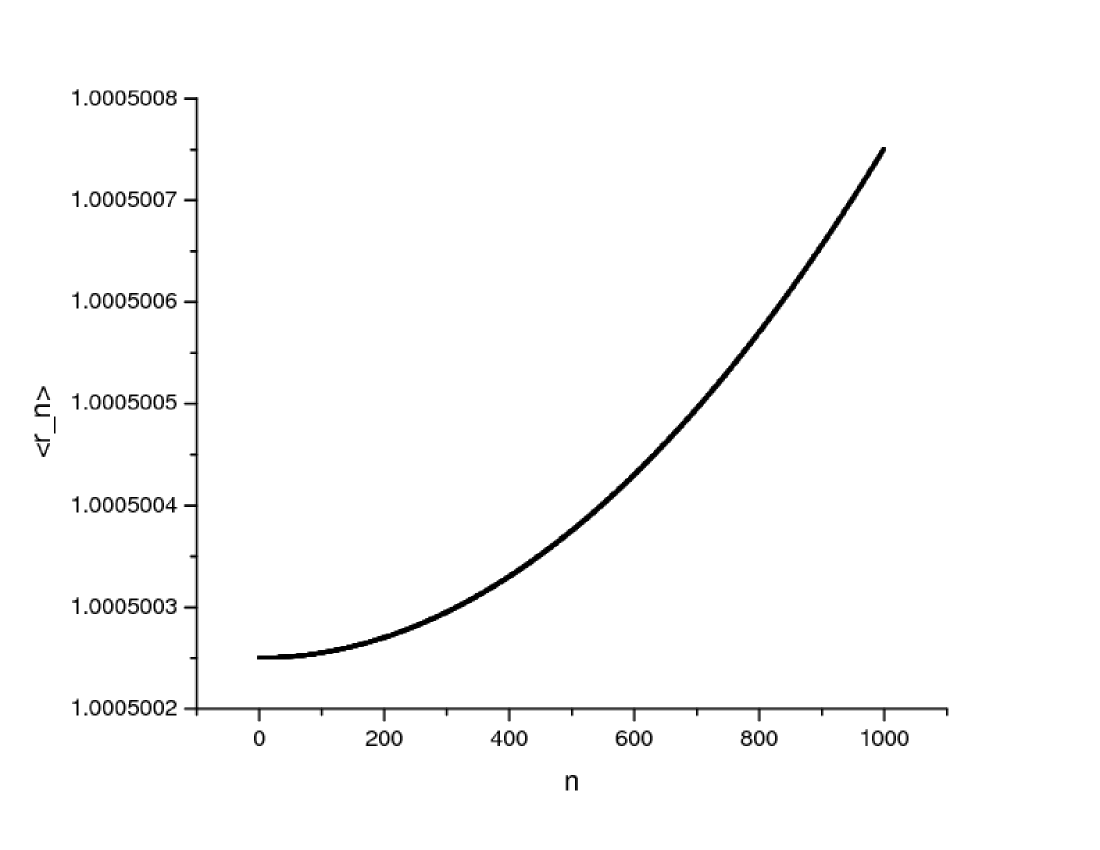
Figure 1: $<r_{n}>$ vs $n$ for $\kappa=-1000,R~{}=~{}1$

It can be seen all the eigenstates are localised within $10^{-2}\%$ of the radius and all of them lie inside shell of thickness of $10^{-5}\%$ of the the radius of the disc. Similar situation is obtained in three dimensions where a ball $B^{3}$ is excised. Now the number of negative energy states is $\propto R^{2}$.

The second example is obtained by the motivation to find out the fate of bound states when the disc is squeezed. For this purpose we consider the case of excising an elliptical disc from ${\mathbb{R}}^{2}$. Separation of variables for the Laplacian is possible if one uses elliptical coordinates which are given in terms of the Cartesian ones by

$$x=a\,\cosh\rho\,\cos\theta,\hskip 21.68121pty=a\,\sinh\rho\,\sin\theta$$ (6)

Here $\rho=\rho_{0}$ corresponds to the elliptical boundary. In these coordinates constant $\rho$ curves are ellipses and constant $\theta$ corresponds to hyperbolae orthogonal to the ellipses. Hence $\rho_{0}\leq\rho<\infty$ and $0\leq\theta<2\pi$. The boundary condition is

$$\left(\partial_{\rho}\psi+\kappa\psi\right)\lvert_{\rho_{0}}=0$$ (7)

Interestingly the number of bound states decreases as we squeeze the circular disc and becomes $\propto a\sinh\rho_{0}$, the minor axis [13]. It is in fact possible to remove all the bound states by squeezing sufficiently to lengths $\leq\frac{1}{\kappa}$. Again the bound states are localised near the boundary.

3 Bose-Einstein condensation

The negative energy bound states in the previous section can create instabilities when a gas of particles at low temperatures is considered in such a manifold. The situation is similar to Bose-Einstein condensate where a divergence in partition function and entropy are prevented by a finite number of particles condensing at low temperatures. To bring out this comparison, we begin with a brief discussion of Bose-Einstein condensation. Although this is standard textbook material, we want to focus attention on some points which can shed light on the problem at hand.

Consider a nonrelativistic gas of bosons, with energy given by $E_{k}=k^{2}/2m$. The partition function is given by $Z={\rm Tr}e^{-\beta(H-\mu N)}$. Normally, we take the states to be of the form

$$|n_{0},n_{k_{1}},n_{k_{2}},\cdots{\rangle}={(a^{\dagger}_{0})^{n_{0}}\over\sqrt{n_{0}!}}\,{(a^{\dagger}_{k_{1}})^{n_{k_{1}}}\over\sqrt{n_{k_{1}}!}}\,{(a^{\dagger}_{k_{2}})^{n_{k_{2}}}\over\sqrt{n_{k_{2}}!}}\,\cdots\,|0{\rangle}$$ (8)

Writing $z=e^{\beta\mu}$ for the fugacity, we find

$$Z=\prod_{k\neq 0}{1\over(1-z\,e^{\beta E_{k}})}~{}{1\over(1-z)}$$ (9)

The fugacity is in the range $0\leq z\leq 1$. Notice that there is a singularity in the partition function (and a corresponding logarithimis singularity in the free energy) as $z\rightarrow 1$. The entropy may be evaluated as

$$S={5\over 2}{V\over\lambda^{3}}\,g_{5\over 2}(z)-\log(1-z),\hskip 21.68121ptg_{\nu}(z)\equiv\sum_{1}^{\infty}{z^{m}\over m^{\nu}}$$ (10)

Here $\lambda=\sqrt{2\pi/mT}$ is the thermal wavelength and $V$ is the volume of the system. There is a singularity in the entropy as well, as $z\rightarrow 1$. This singularity and the divergence of the partition function as $z\rightarrow 1$ is taken as the signal for a phase transition. To understand the nature of this transition, we restrict the total number of particles to be $N$. It is given in terms of the average occupation numbers as

$$N=\sum_{k}{z\over e^{\beta E_{k}}-z}+{z\over 1-z}=\sum_{k}{z\over e^{\beta E_{k}}-z}+{\bar{n}}_{0}$$ (11)

where ${\bar{n}}_{0}=z/(1-z)$ is the average occupation number in the lowest eigenstate of the single-particle Hamiltonian, namely, $k=0$. Working out the integral over $k$, this equation becomes

$$1={V\over N\,\lambda^{3}}g_{3\over 2}(z)+{{\bar{n}}_{0}\over N},$$ (12)

As we lower the temperature, the thermal wavelength $\lambda$ increases, lowering the first term on the righthand side, namely, the contribution of the nonzero modes to this equation. This can be compensated to some extent by an increase of $z$, which also increases $g_{3\over 2}(z)$. However, the maximum value of $g_{3\over 2}(z)$ is at $z=1$, $g_{3\over 2}(z)\leq g_{3\over 2}(1)\approx 2.612$. We see that, at temperatures lower than what is given by this condition, the first term on the right hand side of (12) is less than $1$ and the only way to satisfy (12) is then for ${\bar{n}}_{0}/N$ to be nonzero to make up the deficit. Thus even in the thermodynamic limit of $N\rightarrow\infty$, there is a nonzero fraction (in other words a macroscopically significant number) which must condense into the ground state. The signal for this transition is the singularity in the partition function $Z$ as $z\rightarrow 1$.

The new phase is determined by giving an expectation value to $a_{0}$, corresponding to the lowest energy sigenstate ($E=0$). In other words, rather than states of the form (8), we take them to be of the form

$$|\alpha,n_{k_{1}},n_{k_{2}},\cdots{\rangle} = {(a^{\dagger}_{k_{1}})^{n_{k_{1}}}\over\sqrt{n_{k_{1}}!}}\,{(a^{\dagger}_{k_{2}})^{n_{k_{2}}}\over\sqrt{n_{k_{2}}!}}\,\cdots\,|\alpha,0{\rangle}$$

$$a_{0}\,|\alpha,n_{k_{1}},n_{k_{2}},\cdots{\rangle} = \alpha\,|\alpha,n_{k_{1}},n_{k_{2}},\cdots{\rangle}$$ (13)

Now the partition function and the entropy become

$$\log Z = \alpha^{*}\alpha\,\log z+{V\over\lambda^{3}}\,g_{5\over 2}(z)$$

$$S = {5\over 2}{V\over\lambda^{3}}\,g_{5\over 2}(z)+\alpha^{*}\alpha\,\log z$$ (14)

The equation for the total number of particles is

$$1={V\over N\,\lambda^{3}}g_{3\over 2}(z)+{\alpha^{*}\alpha\over N}$$ (15)

This last equation determines $\alpha$. We will get $\alpha\sim\sqrt{N}\sim\sqrt{V}$, in the thermodynamic limit. We see that there is no singularity in $Z$ or $S$.

The field operator for the particles may be taken as

$$\psi(x)={1\over\sqrt{V}}\sum_{k}a_{k}\,e^{-iE_{k}t+i\vec{k}\cdot{\vec{x}}},\hskip 21.68121pt\psi^{\dagger}(x)={1\over\sqrt{V}}\sum_{k}a_{k}\,e^{iE_{k}t-i\vec{k}\cdot{\vec{x}}}$$ (16)

With $a_{0}\sim\alpha\sim\sqrt{V}$, we see that we get a nonzero value ${\langle}\psi{\rangle}$ for the expectation value of $\psi$ in the ground state of the many-particle system.

It is also useful to consider this in terms of the Euclidean functional integral. Writing

$$\psi(x)=\sum_{-\infty}^{\infty}\,e^{i\omega_{n}\tau}\,q_{n}({\vec{x}})$$ (17)

we find

$$Z=\prod_{n,k}{1\over{\cal E}_{k}+i\omega_{n}}$$ (18)

where ${\cal E}_{k}=E_{k}-\mu$. The sum over Matsubara frequencies in $\log Z$ is divergent. We introduce a Pauli-Villars regulator to write

$${\partial\over\partial{\cal E}_{k}}\log Z=-\sum_{n}\left[{1\over{\cal E}_{k}+i\omega_{n}}-{1\over{\cal E}_{k}+MTi\omega_{n}}\right]$$ (19)

This is easily evaluated and leads to

$$\log Z=-\sum_{k}\left[\log(1-e^{-\beta{\cal E}_{k}})-\log(1-e^{-\beta({\cal E}_{k}+MT)})\right]$$ (20)

When the regulator mass $M$ is taken very large, this reduces to the expression corresponding to $Z$ in (9); thus we mat start from the Euclidean functional integral, obtain (9) and then carry out the rest of the analysis as done above. The main point is that the signal for the transition is seen as a singularity of the Euclidean functional integral. The solution is also given by choosing conditions such that the Euclidean functional integral is well-defined.

Consider now the case where the Laplacian can have negative eigenvalues. It is sufficient to consider just one such mode to illustrate what happens. We denote the corresponding energy eigenvalue as $E=-\lambda_{1}$. The partition function $Z$ is then given by

$$\log Z=-\sum_{k\neq 0}\log(1-ze^{-\beta E_{k}})-\log(1-z)-\log(1-ze^{\beta\lambda_{1}})$$ (21)

We see that we get a singularity even before we get to $z=1$, namely, at $z\,e^{\beta\lambda_{1}}=1$. Once again, we can take this a signaling a phase transition. In fact, taking the states to be of the form

$$|\alpha_{1},n_{0},n_{k_{1}},n_{k_{2}},\cdots{\rangle} = {(a^{\dagger}_{0})^{n_{0}}\over\sqrt{n_{0}!}}{(a^{\dagger}_{k_{1}})^{n_{k_{1}}}\over\sqrt{n_{k_{1}}!}}\,{(a^{\dagger}_{k_{2}})^{n_{k_{2}}}\over\sqrt{n_{k_{2}}!}}\,\cdots\,|\alpha_{1},0{\rangle}$$

$$a_{\lambda_{1}}\,|\alpha_{1},n_{0},n_{k_{1}},n_{k_{2}},\cdots{\rangle} = \alpha_{1}\,|\alpha_{1},n_{0},n_{k_{1}},n_{k_{2}},\cdots{\rangle}$$ (22)

we find

$$\log Z = \alpha_{1}^{*}\alpha_{1}\log(ze^{\beta\lambda})-\log(1-z)+{V\over\lambda^{3}}\,g_{5\over 2}(z)$$

$$1 = {V\over N\,\lambda^{3}}g_{3\over 2}(z)+{z\over(1-z)}+{\alpha_{1}^{*}\alpha_{1}\over N}$$ (23)

The singularity is removed by going to the new phase. We must also consider the value of the fugacity to be in the range $0\leq z\leq z_{1}$, $z_{1}e^{\beta\lambda_{1}}=1$.

Notice that the conservation of particle number is crucial for this. The value of $\alpha_{1}$ have an upper bound by virtue of (23). Without such a constraint, or some such constraint arising from a conserved quantum number (and a corresponding fugacity), we can have an arbitrary number of particles going into the negative energy state and creating a theory with no ground state. This would be the case, for example, for a relativistic massless scalar field. Further, in the relativistic case, the Laplacian occurs under a square root in the expression for the energy. So negative eigenvalues indicate imaginary energies, rather than negative energies. The analysis in such cases will have similarities to the present one, but there will also be differences. We now turn to this problem.

4 Real scalar field

We will start by considering a free scalar field theory for which the the equation of motion, in Euclidean spacetime, is given by

$$\square\,\phi={\partial^{2}\phi\over\partial\tau^{2}}+\nabla^{2}\,\phi=0$$ (24)

Since boundary considerations are important, the first question is to ask what the action is for which this is the equation of motion. This is easily seen to be

$${\cal S}={1\over 2}\int(\partial\phi)^{2}-\oint\partial_{n}\phi\,\phi-{1\over 2}\oint\phi\,{\cal K}\,\phi$$ (25)

The variation of this action gives

$$\delta{\cal S} = \int\delta\phi\,(-\square\phi)-\oint(\partial_{n}\delta\phi+{\cal K}\delta\phi)\,\phi$$ (26)

$$= \int\delta\phi\,(-\square\phi)$$

where we have used the self-adjointness of ${\cal K}$ and we also take fields and their variations to satisfy the condition (2). This shows that ${\cal S}$ is indeed the correct action for the variational derivation of the equations of motion (24).

We can expand the field $\phi$ as

$$\phi(x)=\sum_{A}q_{A}(\tau)\,u_{A}({\vec{x}})$$ (27)

where $q_{A}$ can depend on the imaginary time $\tau$ and the modes $u_{A}({\vec{x}})$ are eigenfunctions of the spatial Laplacian,

$$-\nabla^{2}\,u_{A}({\vec{x}})=\omega_{A}^{2}\,u_{A}({\vec{x}})$$ (28)

The use of the mode expansion (27) reduces the cation to

$${\cal S}={1\over 2}\sum_{A}\,\left({\dot{q}}_{A}^{2}+\omega_{A}^{2}\,q_{A}^{2}\right)$$ (29)

All boundary terms cancel out in the simplification of this expression.

The key point for our analysis is that the eigenvalues $\omega_{A}^{2}$ can be positive or negative. We separate them out as $\{u_{A}\}=(\{u_{\alpha}\},\{u_{a}\})$, with the first set corresponding to positive eigenvalues and the second set to negative eigenvalues,

$$-\nabla^{2}\,u_{\alpha} = \omega_{\alpha}^{2}\,u_{\alpha}$$

$$-\nabla^{2}\,u_{a} = -\lambda_{a}^{2}\,u_{a}$$ (30)

with $\omega_{\alpha}^{2}$ and $\lambda_{a}^{2}$ positive. The action ${\cal S}$ now becomes

$${\cal S}={1\over 2}\sum_{\alpha}\,\left({\dot{q}}_{\alpha}^{2}+\omega_{\alpha}^{2}\,q_{\alpha}^{2}\right)+{1\over 2}\sum_{a}\,\left({\dot{q}}_{a}^{2}-\lambda_{a}^{2}\,q_{a}^{2}\right)$$ (31)

The instability is manifest in the last term; the integration of $e^{-{\cal S}}$ over the variables $q_{a}$ can fail to converge. As mentioned earlier, we will take the standpoint that the theory must be defined by making the Euclidean functional integral well-defined. For this, consider periodic boundary conditions in time $\tau$ with period $\beta=T^{-1}$, $T$ being the temperature. (We use units where the Boltzmann constant $k$ is set to $1$.) Explicitly, we write

$$q_{\alpha}(\tau) = {1\over\sqrt{\beta}}\sum_{n}\,q_{\alpha\,n}\,e^{i\Omega_{n}\tau}$$

$$q_{a}(\tau) = {1\over\sqrt{\beta}}\sum_{n}\,q_{a\,n}\,e^{i\Omega_{n}\tau}$$ (32)

where $\Omega_{n}=2\pi n\,T$. Upon using this in (31), we see that the first term of the action, namely ${\cal S}_{1}$, encounters no difficulties. The second term ${\cal S}_{2}$ becomes

$${\cal S}_{2}=\sum_{a}\sum_{1}^{\infty}\,q^{*}_{a\,n}q_{a\,n}\,(\Omega_{n}^{2}-\lambda_{\alpha}^{2})+{1\over 2}\sum_{a}q_{a\,0}q_{a\,0}(-\lambda_{a}^{2})$$ (33)

We see that we have stability if we make the restrictions that $q_{a\,0}=0$ and that $\Omega_{1}^{2}\geq\Lambda^{2}$, where $-\Lambda^{2}$ is the lowest of the negative eigenvalues. The last condition means that we have stability only if

$$T\geq{\Lambda\over 2\pi}$$ (34)

With these conditions, we can have a well-defined functional integral, the action being given by

$${\cal S}={1\over 2}\sum_{\alpha}\sum_{0}^{\infty}\,q^{*}_{\alpha\,n}q_{\alpha\,n}\,(\Omega_{n}^{2}+\omega_{\alpha}^{2})++{1\over 2}\sum_{a}\sum_{1}^{\infty}\,q^{*}_{a\,n}q_{a\,n}\,(\omega_{n}^{2}-\lambda_{\alpha}^{2})$$ (35)

The functional integration is convergent. However, it is not enough to ensure that the partition function is convergent to avoid pathologies. We have to make sure the propagators are also well behaved. We will consider the calculation of propagators and other correlators to see how a well-defined theory can be obtained. The limit of $T\rightarrow\Lambda/2\pi$ can then be examined to see if there is any phase change.

The propagator for the modes of positive eigenvalues is straightforward and gives

$${\langle}q_{\alpha}(\tau)q_{\beta}(\tau^{\prime}){\rangle} = \delta_{\alpha\beta}{1\over 2\omega_{\alpha}}\left[e^{-\omega_{\alpha}(\tau-\tau^{\prime})}\theta(\tau-\tau^{\prime})+e^{\omega_{\alpha}(\tau-\tau^{\prime})}\theta(\tau^{\prime}-\tau)\right.$$ (36)

$$\hskip 86.72377pt\left.+N_{\omega}\,\left(e^{-\omega_{\alpha}(\tau-\tau^{\prime})}+e^{\omega_{\alpha}(\tau-\tau^{\prime})}\right)\right]$$

This can be continued to Minkowski signature using $\tau-\tau^{\prime}\rightarrow i(t-t^{\prime})$ to get the corresponding correlator in Minkowski space as

$${\langle}q_{\alpha}(t)q_{\beta}(t^{\prime}){\rangle} = \delta_{\alpha\beta}{1\over 2\omega_{\alpha}}\left[e^{-i\omega_{\alpha}(t-t^{\prime})}\theta(t-t^{\prime})+e^{i\omega_{\alpha}(t-t^{\prime})}\theta(t^{\prime}-t)\right.$$ (37)

$$\hskip 86.72377pt\left.+N_{\omega}\,\left(e^{-i\omega_{\alpha}(t-t^{\prime})}+e^{i\omega_{\alpha}(t-t^{\prime})}\right)\right]$$

In (36) and (37),

$$N_{\omega}={1\over e^{\beta\omega_{\alpha}}-1}$$ (38)

These equations are standard, essentially textbook material. We now turn to the negative eigenvalues for which we need to evaluate

$${\langle}q_{a}(\tau)q^{*}_{b}(\tau^{\prime}){\rangle}=\delta_{ab}\,{1\over\beta}\,\sum_{1}^{\infty}e^{i\Omega_{n}(\tau-\tau^{\prime})}{1\over\Omega_{n}^{2}-\lambda_{a}^{2}}$$ (39)

Recall that the sum does not include the $n=0$ mode. This expression can be converted to a contour integral, for $\tau-\tau^{\prime}>0$, as

$${\langle}q_{a}(\tau)q^{*}_{b}(\tau^{\prime}){\rangle}=\delta_{ab}~{}{1\over 2}\left[\oint_{C}{dz\over 2\pi}e^{iz(\tau-\tau^{\prime})}{1\over(z^{2}-\lambda_{a}^{2})(e^{i\beta z}-1)}+{1\over\beta\lambda_{a}^{2}}\right]$$ (40)

where the contour $C$ must enclose all the poles of $(e^{i\beta z}-1)^{-1}$ but not those which arise from $(z^{2}-\lambda_{a}^{2})^{-1}$.

Figure 2: The contour $C$ for the integral in (40)

Figure 3: The contour $C_{1}$ for the integral which gives (41)

Unlike the case for the positive eigenvalues, we now have additional poles on the real axis due to $(z^{2}-\lambda_{a}^{2})^{-1}$. So we choose the contour as shown in Fig. 2. The bold dots are the poles at $z=\pm\lambda_{a}$, which must be outside the contour. The dots at $n=0,\pm 1,\cdots$, are the poles due to $(e^{i\beta z}-1)^{-1}$. We can now extend the contours as much as we like into the imaginary directions, since there are no further poles to worry about. Further, the factor $e^{iz(\tau-\tau^{\prime})}\times(e^{i\beta z}-1)^{-1}$ assures that the integrand falls off exponentially along the imaginary axis. Therefore, we can replace the contour $C$ by the new one $C_{1}$ as shown in Fig. 3.. The contribution is now from the poles at $z=\pm\lambda_{a}$. We then get

$${\langle}q_{a}(\tau)q^{*}_{b}(\tau^{\prime}){\rangle}=\delta_{ab}\left\{{i\over 4\lambda_{a}}\left[{e^{-i\lambda_{a}(\tau-\tau^{\prime})}\over e^{-i\beta\lambda_{a}}-1}-{e^{i\lambda_{a}(\tau-\tau^{\prime})}\over e^{i\beta\lambda_{a}}-1}\right]+{1\over 2\beta\lambda_{a}^{2}}\right\},\hskip 21.68121pt\tau-\tau^{\prime}>0$$ (41)

For $\tau-\tau^{\prime}<0$, we do not obtain the needed fall-off along the imaginary directions using $(e^{i\beta z}-1)^{-1}$. Instead we can use $e^{i\beta z}\times(e^{i\beta z}-1)^{-1}$ which has the same poles and residues as $(e^{i\beta z}-1)^{-1}$. The rest of the analysis is similar to the case of $\tau-\tau^{\prime}>0$ and we get

$${\langle}q_{a}(\tau)q^{*}_{b}(\tau^{\prime}){\rangle}=\delta_{ab}\left\{-{i\over 4\lambda_{a}}\left[{e^{-i\lambda_{a}(\tau-\tau^{\prime})}\over e^{i\beta\lambda_{a}}-1}-{e^{i\lambda_{a}(\tau-\tau^{\prime})}\over e^{-i\beta\lambda_{a}}-1}\right]+{1\over 2\beta\lambda_{a}^{2}}\right\},\hskip 21.68121pt\tau-\tau^{\prime}<0$$ (42)

The two cases (41) and (42) can be combined as

$${\langle}q_{a}(\tau)q^{*}_{b}(\tau^{\prime}){\rangle} = \delta_{ab}\Biggl{\{}{1\over 2\beta\lambda_{a}^{2}}-{1\over 8\,\lambda_{a}\,\sin(\beta\lambda_{a}/2)}\Bigl{[}\exp(-i\lambda_{a}(\tau-\tau^{\prime})\pm i\beta\lambda_{a}/2)$$ (43)

$$\hskip 86.72377pt+\exp(i\lambda_{a}(\tau-\tau^{\prime})\mp i\beta\lambda_{a}/2)\Bigr{]}\Biggr{\}}$$

where the upper sign applies to $\tau-\tau^{\prime}>0$ and the lower to $\tau-\tau^{\prime}<0$. We may rewrite this also as

$${\langle}q_{a}(\tau)q^{*}_{b}(\tau^{\prime}){\rangle}=\delta_{ab}\Biggl{\{}{1\over 2\beta\lambda_{a}^{2}}-{1\over 8\,\lambda_{a}\,\sin(\beta\lambda_{a}/2)}\Bigl{[}\int dp_{0}~{}e^{-ip_{0}(\Delta-\beta/2)}\,\Bigl{(}\delta(p_{0}-\lambda_{a})+\delta(p_{0}+\lambda_{a})\Bigr{)}\Bigr{]}\Biggr{\}}$$ (44)

where $\Delta=\tau-\tau^{\prime}$ and we have only written the case for $\tau-\tau^{\prime}>0$. We can continue this to Minkowski signature by the replacements $p_{0}\rightarrow ip_{0}$, $\Delta\rightarrow i(t-t^{\prime})$. This leads to the Minkowski space expression

$${\langle}q_{a}(t)q^{*}_{b}(t^{\prime}){\rangle}=\delta_{ab}\Biggl{\{}{1\over 2\beta\lambda_{a}^{2}}-{i\over 4\,\sin(\beta\lambda_{a}/2)}\Bigl{[}\int dp_{0}~{}e^{ip_{0}(t-t^{\prime})\mp p_{0}\beta/2}\,\,\delta(p_{0}^{2}+\lambda_{a}^{2})\Bigr{]}\Biggr{\}}$$ (45)

We see that there is an exponentially growing part to this and hence there is an instability in processes if we couple this to external sources and consider, for example, a scattering problem. This can be avoided if we make the following additional rule:

Observer has access only to the modes $q_{\alpha\,n}$, corresponding to the positive eigenvalues.

Thus in any Feynman diagram, we cannot have $q_{a\,n}$ in the external lines or coupling to sources.

We might also worry about possible singularities because of the $\sin(\beta\lambda_{a}/2)$ in the denominator in (45). This can happen for $T=\lambda_{a}/2\pi n$. All such values are excluded already by (34), except for $n=1$ and $\lambda_{a}=\Lambda$. This last point is the limit of the inequality in (34). It is also excluded if we postulate an unattainability rule that the inequality in (34) cannot be saturated, something like a new third law of thermodynamics. Our conclusion is that the Euclidean functional is well-defined and the Minkowski continuation of correlators can be meaningfully interpreted if we make the restrictions:

1. $q_{a\,0}=0$

2. $T>{\Lambda\over 2\pi}$, with the limit $T={\Lambda\over 2\pi}$ unattainable

3. Observers have access only to the modes $q_{\alpha}$, not to $q_{a}$. However, $q_{a}$ can contribute to processes via loops.

We now return to thermodynamic considerations, calculating the free energy and the entropy due to the unstable modes. For the contribution to the free energy, we may write

$$\beta\,F=\sum_{a}\sum_{1}^{\infty}\,\log(\Omega_{n}^{2}-\lambda_{a}^{2})$$ (46)

Differentiating with respect to $\lambda_{a}$ we get a sum similar to what was obtained for the propagators. Carrying out the summation with the same contour integration techniques, and integrating over $\lambda_{a}$, we find

$$\beta\,F=\sum_{a}\left[-\log\lambda_{a}+\log\left(2i\sin(\beta\lambda_{a}/2)\right)+(\lambda_{a}{\rm-independent~{}term})\right]$$ (47)

The constant term can be identified by looking at small values of $\beta\lambda_{a}$. This leads to

$$F={1\over\beta}\sum_{a}\,\log\left[{\sin(\beta\lambda_{a}/2)\over(\beta\lambda_{a}/2)}\right]$$ (48)

The entropy can be calculated as

$$S=1+\sum_{a}\,\log\left[{\sin(\beta\lambda_{a}/2)\over(\beta\lambda_{a}/2)}\right]-\sum_{a}{\beta\lambda_{a}\over 2}\cot(\beta\lambda_{a}/2)$$ (49)

In both the free energy and the entropy, there is a singularity as $\beta\lambda_{a}\rightarrow 2\pi$. For $\beta\lambda_{a}=2(\pi-\epsilon)$,

$$F \rightarrow {1\over\beta}\log(\epsilon/\pi)$$

$$S \rightarrow {\pi\over\epsilon}+\log\epsilon$$ (50)

We take this as signaling a phase transition. We could consider the field as developing an expectation value. However, unlike the case discussed in section 2, we do not have a conservation law for the particle number and hence there is no equation which can serve to determine the expectation value. This is the same problem as in the Bose-Einstein condensation of a free relativistic massless scalar field; the action is of the form ${\cal S}={\textstyle{1\over 2}}\int(\partial\phi)^{2}$and the theory can exist in a phase with ${\langle}\phi{\rangle}=$ any constant value. If there are interactions, such as a $\phi^{4}$-term, then the interaction will eventually serve to determine ${\langle}\phi{\rangle}$. This is also the case for a theory with a negative (mass)² term, which is closer to the situation we have. Mass corrections can generically boost the negative eigenvalues to positive or zero values. In the context of the $\delta$-function potentials mentioned in the introduction, such a mechanism has been studied in [7] and also in [14]. (See also the added reference [15].) So to analyze this possibility, we will now consider possible mass corrections arising from a $\phi^{4}$-interaction.

5 The interacting theory

The action for the interacting theory will be taken to be

$${\cal S}=\sum_{\alpha}\sum_{1}^{\infty}\,q^{*}_{\alpha\,n}q_{\alpha\,n}\,(\Omega_{n}^{2}+\omega_{\alpha}^{2})+{1\over 2}\sum_{\alpha}q_{\alpha\,0}^{2}\,\omega_{\alpha}^{2}+\sum_{a}\sum_{1}^{\infty}\,q^{*}_{a\,n}q_{a\,n}\,(\Omega_{n}^{2}-\lambda_{a}^{2})+g\int\phi^{4}$$ (51)

We will separate out the unstable modes by writing $\phi={\varphi}+\eta$, where

$${\varphi}={1\over\sqrt{\beta}}\sum q_{\alpha\,n}e^{i\Omega_{n}\tau}\,u_{\alpha}({\vec{x}}),\hskip 21.68121pt\eta={1\over\sqrt{\beta}}\sum q_{a\,n}e^{i\Omega_{n}\tau}\,u_{a}({\vec{x}})$$ (52)

The strategy is to integrate out the $\eta$’s to obtain an effective action for the ${\varphi}$’s. This result can then be continued to Minkowski space and real-time processes can be calculated. So long as there are no sources coupled to the unstable modes, $\eta$’s only contribute in loops and this process can be consistently implemented.

First of all, let us consider tree-graphs where the $\eta$-propagator can occur. The question is whether these can lead to new instabilities requiring new restrictions. Consider as an example the term $\int{\varphi}(x)^{3}\,{\langle}\eta(x)\eta(y){\rangle}\,{\varphi}(y)^{3}$. Using the expression for the propagator in (44), this can be evaluated in a straightforward manner as

$$\int{\varphi}(x)^{3}\,{\langle}\eta(x)\eta(y){\rangle}\,{\varphi}(y)^{3}=\int d^{4}xd^{4}y~{}{\varphi}(x)^{3}\,V(x,y)\,{\varphi}(y)^{3}$$ (53)

where

$$V(x,y)=\sum_{a}u_{a}({\vec{x}})\,u_{a}^{*}(\vec{y})\,\int{d\omega\over 2\pi}{d\omega^{\prime}\over 2\pi}\,e^{i\omega x^{0}+i\omega^{\prime}y^{0}}\left[{(2\pi)^{2}\delta(\omega)\delta(\omega^{\prime})\over 2\beta\lambda_{a}^{2}}-{2\pi\delta(\omega+\omega^{\prime})\over 2(\omega^{2}+\lambda_{a}^{2})}\right]$$ (54)

There is nothing pathological about this. Notice that the first term in $V(x,y)$ is an instantaneous potential which is also temperature-dependent. It is confined to a region close to the boundary since the $u_{a}({\vec{x}})$ fall off as we move away from the boundary. Turning to loop corrections, the simplest one we can evaluate is the one-loop mass correction due to the unstable modes. This is easily seen to be given by

$$\Delta{\cal S} = {1\over 2}\int V(x)\,{\varphi}^{2}(x)$$

$$V(x) = 12g\sum_{a}u_{a}({\vec{x}})\,u^{*}_{a}({\vec{x}})\left[{1\over 2\beta\lambda_{a}^{2}}-{1\over 4\lambda_{a}}\cot(\beta\lambda_{a}/2)\right]$$ (55)

Being a position-dependent mass term, this is really a single-particle potential for the ${\varphi}$ modes. $V(x)$ is again concentrated near the boundary. It is positive for all values of $\beta\lambda_{a}$ in the range of interest. Thus ${\varphi}$’s experience a repulsive potential near the boundary helping to avoid any further instabilities, at least to this order.

Let us now consider the thermodynamic quantities. The partition function will get contributions from diagrams of the type shown in Fig. 4, where the propagators are those corresponding to the unstable modes $\eta$. The first term is the free part which gives the expressions (48) and (49).

Figure 4: Diagrams involving the propagator of the unstable modes which contribute to the partition function

The extra loops correspond to the modification of the propagator via a mass correction for the $\eta$ fields. So while this does not have to be taken account of in external lines, this mass correction does influence the thermodynamics. Evidently, the mass correction for this is of the form ${\textstyle{1\over 2}}\int V(x)\,\eta^{2}$. Thus the effect of the series is to change the expression for the free energy to

$$\beta\,F=\sum_{a}\sum_{1}^{\infty}\log(\Omega_{n}^{2}-{\tilde{\lambda}}_{a}^{2})$$ (56)

where $\tilde{\lambda}_{a}$ are the eigenvalues of $-\nabla^{2}+V(x)$,

$$(-\nabla^{2}+V(x))\,{\tilde{u}}_{a}=-{\tilde{\lambda}}_{a}^{2}\,{\tilde{u}}_{a}$$ (57)

with $V(x)$ as given in (55). This extra repulsive potential can make the eigenvalues $-{\tilde{\lambda}}_{a}^{2}$ positive avoiding the singularity as $\beta\lambda_{a}\rightarrow 2\pi$. Unfortunately, an explicit calculation is rather difficult, since the potential $V(x)$ diverges as $\beta\lambda_{a}\rightarrow 2\pi$, making any perturbative evaluation of corrections inadequate. Nevertheless, it is useful to get an estimate of the correction to the eigenvalues in perturbation theory, say, to first order. For the example introduced in Sec. 2 of ${\mathbb{R}}^{2}$ with a disc of radius $R$ excised from it, consider the case when we have only one eigenstate with negative eigenvalue. This can be obtained for $\kappa R=0.5$ for example. Taking this as an illustrative case, we find $z_{*}\approx 0.165725$ and the eigenfunction is

$$u(x) = (2\pi R^{2}{\cal I})^{-1/2}\,K_{0}(z_{*}r/R)$$

$${\cal I} = \int_{1}^{\infty}dw\,w\,(K_{0}(z_{*}w))^{2}$$ (58)

The eigenvalue $-z_{*}^{2}/R^{2}$, with the first correction included becomes

$$-{\tilde{\lambda}}^{2}\approx{z_{*}^{2}\over R^{2}}\left[-1+(0.2102)\times{3\,g\over\lambda}\left[{1\over(\beta\lambda/2)}-\cot(\beta\lambda/2)\right]\right]$$ (59)

The correction is not small except for very small $g$ and $\beta\lambda$, and diverges as $\beta\lambda\rightarrow 2\pi$, showing that the negative modes are eliminated before we get to $\beta\lambda=2\pi$. As mentioned above, perturbation theory is not adequate for this analysis; we plan to explore a numerical approach to this question in future.

6 Discussion

In this paper we have considered field theories on manifolds with boundaries and for which the one-particle kinetic energy operator, taken as the Laplacian, has negative eigenvalues. The possibility of negative eigenvalues is related to the choice of boundary conditions. The general theory shows that there is a large class of boundary conditions, in fact infinitesimally close to standard and well-known ones such as Dirichlet and Neumann, for which the Laplacian can have negative eigenvalues. Explicit illustrative examples were given in Sec. 2. Our strategy for analyzing such theories was to start with defining the theory at finite and high enough temperature for which we have a well-defined partition function and then pose the question of whether we can lower the temperature to zero. The analysis leads to three different cases.

If we consider free field theories with a conserved particle number operator, there is Bose-Einstein condensation as we lower the temperature with a thermodynamically nontrivial fraction condensing into the mode with the lowest (and negative) eigenvalue for the Laplacian; the transition temperature is related to this lowest eigenvalue. Stability in this case is due to the total number of particles being fixed.

By contrast, if we consider a real scalar field, for which there is no conserved number operator (and hence no corresponding chemical potential), we find that a stable theory is possible only if the temperature remains above a certain value $\Lambda/2\pi$, where $-\Lambda^{2}$ is the lowest eigenvalue of the Laplacian. The temperature $\Lambda/2\pi$ plays the role of absolute zero for this case, with a corresponding unattainability condition (as in the usual third law of thermodynamics). Further, observers should have access only to the modes with positive eigenvalues. These features, particularly the fact that the system shows finite temperature and that the modes of negative eigenvalues are localized near the boundary, are very suggestive of what is observed in the region outside the horizon of a black hole. At this point, this is still an intriguing analogy; the possibility of a deeper connection is worth exploring. As the temperature approaches the value $\Lambda/2\pi$, thermodynamic quantities such as the free energy and entropy diverge again suggesting a phase transition. However, within the free theory, there is no way to determine the expectation value for the field.

The third case of interest, which is also related to the second case, is when we have an interacting scalar field theory. We considered a simple example of a $\phi^{4}$-type interaction. The modes with negative eigenvalues can contribute in loops and the general effect is to create a new repulsive potential near the boundary. We expect this to eliminate the negative eigenvalues and lead to a stable theory as the temperature approaches the critical value $\Lambda/2\pi$. The extra potential diverges as this limit is approached, making any perturbative analysis nonviable. We plan to explore this question is more detail numerically in future work.

The addition of ‘mass term’ on the boundary would presumably save the thermodynamic quantities such as the free energy. But the negative energy modes localised at the boundary remain as ‘zero energy’ modes. The lesson is there could be edge states localised at the boundary even in conventional circumstances. But under perturbation through interactions they will go away since there is ‘no gap’ with bulk modes. But with new boundary conditions which have global origin they will remain stable. This will be seen in the behaviour of two-point functions of the edge modes.

Lastly we would like to remark about fermionic theories . The Dirac operator on such manifolds have to be supplemented by Atiyah, Patodi and Singer global boundary conditions [16] in order to be self adjoint. The square of the Dirac operator is positive definite. But edge states localised on the boundary persists, see for example [12]. This can change thermodynamics, a question which we plan to explore in future.

After this paper was written, we became aware of [15] where a specific realization of the negative eigenvalues is used as a possible mechanism for breaking gauge symmetries. (We thank S. Ohya fro bringing this work to our attention.) Our analysis is quite different, even though there are some points of overlap. We consider the question of how the scalar field self-interactions affect the whole issue of condensation to be not settled in that case as well. Acknowledgements

We thank Professor A.P. Balachandran for discussions. TRG would like to thank Manuelo Asorey for sharing his insights.

This research was also supported by the U.S. National Science Foundation grant PHY-1213380 and by a PSC-CUNY award.

References

- [1] J. von Neumann, Math. Ann. 102 49 (1929).
- [2] M. Asorey, A.Ibort and G. Marmo, “Global theory of quantum boundary conditions and topology change”, Int. J. Mod. Phys. A20 1001 (2005); M. Asorey, D. Garcia-Alvarez, J. M. Munoz-Castaneda, “Casimir Effect and Global Theory of Boundary Conditions”, J. Phys. A39 6127 (2006); M. Asorey, J. M. Munoz-Castaneda, “Vacuum Boundary Effects”, J. Phys. A41 304004 (2008).
- [3] Berry, M V 2009, ’Hermitian boundary conditions at a Dirichlet singularity: the Marletta-Rozenblum model’, J. Phys. A 42 165208.
- [4] T.R. Govindarajan and R. Tibrewala, Phys. Rev. D 83, 124045 (2011)
- [5] M. Asorey and J.M. Munoz-Castaneda, Nucl. Phys. B 874, 852 (2013)
- [6] D. Karabali and V.P.Nair, Phys. Rev. D 87, 105021 (2013)
- [7] J.M. Munoz-Castaneda, J.M. Guilarte and A.M. Mosquera, Phys. Rev. D 87, 105020 (2013)
- [8] P. Parashar, K.A. Milton, K.V. Shajesh and M. Schaden, Phys. Rev. D 86, 085021 (2012)
- [9] M. Bordag, Phys. Rev. D 70 085010 (2004); M. Bordag and D. Vassilevich, Phys. Rev. D 70, 045003 (2004); see also, M. Bordag, J. Phys. A 25, 4483 (1992)
- [10] A.P. Balachandran, L. Chandar, E. Ercolessi, T.R. Govindarajan and R. Shankar, Int. J. Mod. Phys. A09, 3417 (1994); T.R. Govindarajan, V. Suneeta, S. Vaidya, Nucl.Phys. B583 291 (2000).
- [11] I.G. Avramidi and G. Esposito, Class. Quant. Grav. 15, 281 (1998).
- [12] M. Asorey, A.P. Balachandran, J.M. Perez-Pardo, Edge States: Topological Insulators, Superconductors and QCD Chiral Bags
- [13] T R Govindarajan, R Parthasarathy and R Tibrewala (under preparation) arXiv:1308.5635.
- [14] J.M. Guilarte and J.M. Munoz-Castaneda, Int. J. Theor. Phys. 50, 2227 (2011).
- [15] Yukihiro Fujimoto, Tomoaki Nagasawa, Satoshi Ohya, Makoto Sakamoto, Prog. Theor. Phys. 126, 841 (2011).
- [16] M. F Atiyah, V. K Patodi and I. M Singer, Spectral asymmetry and Riemannian Geometry I, Mathematical Proceedings of the Cambridge Philosophical Society, 77 43 (1975).