Codebook-Based Opportunistic Interference Alignment

Abstract

Opportunistic interference alignment (OIA) asymptotically achieves the optimal degrees-of-freedom (DoF) in interfering multiple-access channels (IMACs) in a distributed fashion, as a certain user scaling condition is satisfied. For the multiple-input multiple-output IMAC, it was shown that the singular value decomposition (SVD)-based beamforming at the users fundamentally reduces the user scaling condition required to achieve any target DoF compared to that for the single-input multiple-output IMAC. In this paper, we tackle two practical challenges of the existing SVD-based OIA: 1) the need of full feedforward of the selected users’ beamforming weight vectors and 2) a low rate achieved based on the exiting zero-forcing (ZF) receiver. We first propose a codebook-based OIA, in which the weight vectors are chosen from a pre-defined codebook with a finite size so that information of the weight vectors can be sent to the belonging BS with limited feedforward. We derive the codebook size required to achieve the same user scaling condition as the SVD-based OIA case for both Grassmannian and random codebooks. Surprisingly, it is shown that the derived codebook size is the same for the two considered codebook approaches. Second, we take into account an enhanced receiver at the base stations (BSs) in pursuit of improving the achievable rate based on the ZF receiver. Assuming no collaboration between the BSs, the interfering links between a BS and the selected users in neighboring cells are difficult to be acquired at the belonging BS. We propose the use of a simple minimum Euclidean distance receiver operating with no information of the interfering links. With the help of the OIA, we show that this new receiver asymptotically achieves the channel capacity as the number of users increases.

I Introduction

Interference alignment (IA) [1, 2] is the key ingredient to achieve the optimal degrees-of-freedom (DoF) for a variety of interference channel models. The conventional IA framework, however, has several well-known practical challenges: global channel state information (CSI) and arbitrarily large frequency/time-domain dimension extension. Recently, the concept of opportunistic interference alignment (OIA) was introduced in [3, 4], for the $K$-cell single-input multiple-output (SIMO) interfering multiple-access channel (IMAC), where there are one $M$-antenna base station and $N$ users in each cell. In the OIA scheme for the SIMO IMAC, $S$ ($S\leq M$) users amongst the $N$ users are opportunistically selected in each cell in the sense that inter-cell interference is aligned at a pre-defined interference space. Even if several studies have independently addressed one or a few of the practical problems (see [5, 6]), the OIA scheme simultaneously resolves the aforementioned issues. Specifically, the OIA scheme operates with i) local CSI acquired via pilot signaling, ii) no dimension extension in the time/frequency domain, iii) no iterative optimization of precoders, and iv) no coordination between the users or the BSs. It has been shown that there exists a trade-off between the the achievable DoF and the number of users, which can be characterized by a user scaling condition [4, 7, 8]. Similarly, the analysis of the scaling condition of some system parameters required to achieve a target performance have been widely studied to provide a remarkable insight into the convergence rate to the target performance, e.g., the user scaling condition to achieve target DoF for the IMAC [3, 4, 7, 8], the scaling condition of the number of feedback bits to achieve the optimal DoF for multiple-input multiple-output (MIMO) interference channels [9, 10], and the codebook size scaling condition to achieve the target achievable rate for limited feedback MIMO systems [11, 12, 13]. For the SIMO IMAC, the OIA scheme asymptotically achieves $KS$ DoF, for $0<S\leq M$, if the number of per-cell users, $N$, scales faster than $\textrm{SNR}^{(K-1)S}$ [4], where SNR denotes the received signal-to-noise ratio (SNR). Note that the optimal DoF is achieved when $S=M$.

For the MIMO IMAC, where each user has $L$ antennas, the user scaling condition to achieve $KS$ DoF can be greatly reduced to $\textrm{SNR}^{(K-1)S-L+1}$ with the use of singular value decomposition (SVD)-based beamforming at each user, by further minimizing the generating interference level [7]. However, to implement the SVD-based OIA with local CSI and no coordination between the users or the BSs, each beamforming weight vector is computed at each user, and then information of the selected users’ weight vectors should be sent to the corresponding BS for the coherent detection. In addition, although the OIA based on the zero-forcing (ZF) receiver at the BSs is sufficient to achieve the optimal DoF, its achievable rate is in general far below the channel capacity, and the gap increases as the dimension of channel matrices grows. In this paper, we would like to answer the aforementioned two practical issues of the SVD-based OIA.

In recent cellular systems such as the 3GPP Long Term Evolution [14], each selected user should transmit an uplink pilot (known as Sounding Reference Signal in 3GPP systems) so that the corresponding BS estimates the uplink channel matrix, which is widely used for channel quality estimation, downlink signal design assuming the channel reciprocity in time division duplexing (TDD) systems, etc. The effective channel matrices rotated by the weight vectors should also be known so that the BSs perform coherent detection—the matrices can be acquired by the BSs through either of the following two methods: i) additional dedicated time/frequency pilot (known as Demodulation Reference Signal in 3GPP systems [14]), where the pilots are rotated by weight vectors [15, 16] and ii) limited feedforward of the indices of the weight vectors (as included in Downlink Control Information Format 4 [17]). For the first method, however, the system capacity can be degraded as the number of selected users increases due to the increased pilot overhead [18, 19]. For a reliable transmission, the length of pilot signaling also needs to be sufficiently long [20, 21]. Furthermore, in cellular networks, long training sequences or disjoint pilot resources for all users in each cell are required to avoid the pilot contamination coming from the inter-cell interference [22]. For these reasons, practical communication systems such as the 3GPP standard allow highly limited resources for uplink pilot. On the other hand, the second method using the limited feedforward is preferable especially for the MIMO IMAC in the sense that feedforward information can be flexibly multiplexed with uplink data requiring no additional pilot resource. Several studies [18, 19, 23] have addressed the same issues on the feedforward of the weight vectors for multiuser MIMO systems, and have proposed the design of codebook-based precoding matrices.

In the first part of this paper, we introduce a codebook-based OIA scheme, where weight vectors are chosen from a pre-defined codebook with a finite size such that information of the weight vectors of selected users is sent to the corresponding BS via limited feedforward signaling. Two widely-used codebooks, the Grassmannian and random codebooks, are used. Surprisingly, although the granularity of the Grassmannian codebook is higher than that of the random codebook for a given codebook size, our result indicates that for both codebook approaches, the codebook size, required to achieve the same user scaling condition as the SVD-based OIA case, coincides. It is also shown that the required codebook size in bits increases linearly with the number of transmit antennas and logarithmically with the received SNR, i.e., the required codebook size scales as $L\operatorname{log}_{2}\textrm{SNR}$.

In the second part, we propose a receiver design at the BSs in pursuit of improving the achievable rate based on the ZF receiver. The design is challenging in the sense that local CSI and no coordination between any BSs are assumed, thus resulting in no available information of the interfering links at each BS. Thus, the maximum likelihood (ML) decoding is not possible at each BS since the covariance matrix of the effective noise cannot be estimated due to no information of the interfering links. We propose the use of a simple minimum Euclidean distance receiver, where the ML cost-function is used by assuming the identity noise covariance matrix, which does not require information of the interfering links. We show that this receiver asymptotically achieves the channel capacity as the number of users increases.

Simulation results are provided to justify the derived user and codebook size scaling conditions and to evaluate the performance of the minimum Euclidean distance receiver. A practical scenario, e.g., low SNR, small codebook size, and a small number of users, is taken into account to show the robustness of our scheme.

The remainder of this paper is organized as follows. Section II describes the system and channel models and Section III presents the proposed codebook-based OIA scheme. Section IV derives the user and codebook size scaling conditions of the proposed OIA scheme along with two different codebooks and Section V derives the asymptotic performance of the minimum Euclidean distance receiver. Section VI performs the numerical evaluation. Section VII summarizes the paper with some concluding remarks.

Notations: $\mathbb{C}$ indicates the field of complex numbers. $(\cdot)^{\textrm{T}}$ and $(\cdot)^{\textrm{H}}$ denote the transpose and the conjugate transpose, respectively. $\mathbf{I}_{n}$ is the $(n\times n)$-dimensional identity matrix.

II System and Channel Models

Consider the TDD MIMO IMAC with $K$ cells, each of which consists of a BS with $M$ antennas and $N$ users, each having $L$ antennas, as depicted in Fig. 1. It is assumed that each selected user transmits a single spatial stream. In each cell, $S$ ($S\leq M$) users are selected for uplink transmission. Let $\mathbf{H}_{k}^{[i,j]}\in\mathbb{C}^{M\times L}$ denote the channel matrix from user $j$ in the $i$th cell to BS $k$. A frequency-flat fading and the reciprocity between uplink and downlink channels are assumed. Each element of $\mathbf{H}_{k}^{[i,j]}$ is assumed to be an identical and independent complex Gaussian random variable with zero mean and variance $1/L$. User $j$ in the $i$th cell estimates the uplink channel of its own link, $\mathbf{H}^{[i,j]}_{k}$ ($k=1,\ldots,K$), via downlink pilot signaling transmitted from the BSs; that is, local CSI is utilized as in [6]. Without loss of generality, the indices of the selected users in each cell are assumed to be $(1,\ldots,S)$ for notational simplicity. Then, the received signal at BS $i$ is expressed as:

$$\mathbf{y}_{i} =\sum_{j=1}^{S}\mathbf{H}_{i}^{[i,j]}\mathbf{w}^{[i,j]}x^{[i,j]}+\underbrace{\sum_{k=1,k\neq i}^{K}\sum_{m=1}^{S}\mathbf{H}_{i}^{[k,m]}\mathbf{w}^{[k,m]}x^{[k,m]}}_{\textrm{inter-cell interference}}+\mathbf{z}_{i},$$ (1)

where $\mathbf{w}^{[i,j]}\in\mathbb{C}^{L\times 1}$ and $x^{[i,j]}$ are the weight vector and transmit symbol with unit average power at user $j$ in the $i$th cell, respectively, and $\mathbf{z}_{i}\in\mathbb{C}^{M\times 1}$ denotes the additive white Gaussian noise at BS $i$, with zero mean and the covariance $N_{0}\mathbf{I}_{M}$.

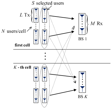
Figure 1: The MIMO IMAC model.

III Proposed Codebook-Based OIA: Overall Procedure

The proposed scheme essentially follows the same procedure as that of the SVD-based MIMO OIA [7, 8] except for the weight vector design step. For the completeness of our achievability results, we briefly describe the overall procedure for all the steps.

III-A Offline Procedure - Reference Basis Broadcasting

The orthogonal reference basis matrix at BS $k$, to which the received interference vectors are aligned, is denoted by $\mathbf{Q}_{k}=\left[\mathbf{q}_{k,1},\ldots,\mathbf{q}_{k,M-S}\right]\in\mathbb{C}^{M\times(M-S)}$. Here, BS $k$ in the $k$th cell ($k\in\{1,\ldots,K\}$) independently and randomly generates $\mathbf{q}_{k,m}\in\mathbb{C}^{M\times 1}$ ($m=1,\ldots,M-S$) from the $M$-dimensional sphere. BS $k$ also finds the null space of $\mathbf{Q}_{k}$, defined by $\mathbf{U}_{k}=\left[\mathbf{u}_{k,1},\ldots,\mathbf{u}_{k,S}\right]\triangleq\textrm{null}(\mathbf{Q}_{k})$, where $\mathbf{u}_{k,i}\in\mathbb{C}^{M\times 1}$ is orthonormal, and then broadcasts it to all users. Note that this process is required only once prior to data transmission and does not need to change with respect to channel instances.

III-B Step 1 - Weight Vector Design

Let us denote the codebook set consisting of $N_{f}$ elements as $\mathcal{C}_{f}\triangleq\left\{\mathbf{c}_{1},\ldots,\mathbf{c}_{N_{f}}\right\}$, where $\mathbf{c}_{1},\ldots,\mathbf{c}_{N_{f}}\in\mathbb{C}^{L\times 1}$ are chosen from the $L$-dimensional unit sphere. Then, the number of bits to represent $\mathcal{C}_{f}$ is denoted by $n_{f}=\lceil\operatorname{log}_{2}N_{f}\rceil$. Let $\mathbf{w}^{[i,j]}$ denote the weight vector at user $j$ in the $i$th cell. Each user attempts to minimize the leakage of interference (LIF) $\eta^{[i,j]}$ defined by [4, 7]

$$\eta^{[i,j]}=\sum_{k=1,k\neq i}^{K}\left\|\mathbf{U}_{k}^{\textrm{H}}\mathbf{H}_{k}^{[i,j]}\mathbf{w}^{[i,j]}\right\|^{2}=\left\|\mathbf{G}^{[i,j]}\mathbf{w}^{[i,j]}\right\|^{2},$$ (2)

where $\mathbf{G}^{[i,j]}$ is the stacked interference channel matrix given by

$$\mathbf{G}^{[i,j]} \triangleq\Big{[}\left({\mathbf{U}_{1}}^{\textrm{H}}\mathbf{H}_{1}^{[i,j]}\right)^{\textrm{T}},\ldots,\left({\mathbf{U}_{i-1}}^{\textrm{H}}\mathbf{H}_{i-1}^{[i,j]}\right)^{\textrm{T}},\left({\mathbf{U}_{i+1}}^{\textrm{H}}\mathbf{H}_{i+1}^{[i,j]}\right)^{\textrm{T}},\ldots,\left({\mathbf{U}_{K}}^{\textrm{H}}\mathbf{H}_{K}^{[i,j]}\right)^{\textrm{T}}\Big{]}^{\textrm{T}}.$$ (3)

Let us denote the SVD of $\mathbf{G}^{[i,j]}$ by $\mathbf{G}^{[i,j]}=\mathbf{E}^{[i,j]}\boldsymbol{\Sigma}^{[i,j]}{\mathbf{V}^{[i,j]}}^{\textrm{H}}$, where $\mathbf{E}^{[i,j]}\in\mathbb{C}^{(K-1)S\times L}$ and $\mathbf{V}^{[i,j]}\in\mathbb{C}^{L\times L}$ are left- and right-singular vectors of $\mathbf{G}^{[i,j]}$, respectively, consisting of $L$ orthonormal columns, and $\boldsymbol{\Sigma}^{[i,j]}=\textrm{diag}\left(\sigma^{[i,j]}_{1},\ldots,\sigma^{[i,j]}_{L}\right)$. Here, $\sigma^{[i,j]}_{m}$ denotes the $m$th singular value of $\mathbf{G}^{[i,j]}$, where $\sigma^{[i,j]}_{1}\geq\cdots\geq\sigma^{[i,j]}_{L}$. Then, $\mathbf{w}^{[i,j]}$ is obtained from $\mathbf{w}^{[i,j]}=\operatorname{arg}\operatorname{max}_{1\leq n\leq N_{f}}\left|\left(\mathbf{v}_{L}^{[i,j]}\right)^{H}\mathbf{c}_{n}\right|^{2}$. Clearly, the weight vector minimizing $\eta^{[i,j]}$ is the $L$th column of $\mathbf{V}^{[i,j]}$, denoted by $\mathbf{v}_{L}^{[i,j]}$, and this precoding is subject to the SVD-based OIA.

III-C Step 2 - User Selection

Each user reports its LIF metric in (2) to the corresponding BS, and then each BS selects $S$ users, having the LIF metrics up to the $S$th smallest one, amongst $N$ users in the cell. Subsequently, each selected user forwards the index of $\mathbf{w}^{[i,j]}$ in the codebook to the belonging BS.

III-D Step 3 - Uplink Transmission and Detection

If all the selected users transmit the uplink signals simultaneously, then the received signal at BS $i$ is given by (1). As in the SVD-based OIA [7], the linear ZF detection is sufficient to achieve the maximum DoF. The decision statistics $\mathbf{r}_{i}$ at BS $i$ is obtained from

$$\mathbf{r}_{i}=\left[r_{i,1},\ldots,r_{i,S}\right]^{\textrm{T}}\triangleq{\mathbf{F}_{i}}^{\textrm{H}}\mathbf{U}_{i}^{\textrm{H}}\mathbf{y}_{i},$$ (4)

where $\mathbf{F}_{i}\in\mathbb{C}^{S\times S}$ is the ZF equalizer defined by

$$\mathbf{F}_{i} =\left[\mathbf{f}_{i,1},\ldots,\mathbf{f}_{i,S}\right]$$

$$\triangleq\left(\left[{\mathbf{U}_{i}}^{\textrm{H}}\mathbf{H}_{i}^{[i,1]}\mathbf{w}^{[i,1]},\ldots,{\mathbf{U}_{i}}^{\textrm{H}}\mathbf{H}_{i}^{[i,S]}\mathbf{w}^{[i,S]}\right]^{-1}\right)^{\textrm{H}}.$$

Note that multiplying ${\mathbf{U}_{i}}^{\textrm{H}}$ to $\mathbf{y}_{i}$ cancels interference aligned at $\mathbf{Q}_{i}$. The achievable rate $R^{[i,j]}$ is then given by

$$R^{[i,j]} \!=\!\operatorname{log}_{2}\left(1+\textrm{SINR}^{[i,j]}\right)\!=\!\operatorname{log}_{2}\left(1+\frac{\textrm{SNR}}{\left\|\mathbf{f}_{i,j}\right\|^{2}\!+\!\tilde{I}^{[i,j]}}\right),$$ (5)

where $\textrm{SNR}=1/N_{0}$ and $\tilde{I}^{[i,j]}\triangleq\sum_{k=1,k\neq i}^{K}\sum_{m=1}^{S}\left|{\mathbf{f}_{i,j}}^{\textrm{H}}{\mathbf{U}_{i}}^{\textrm{H}}\mathbf{H}_{i}^{[k,m]}\mathbf{w}^{[k,m]}\right|^{2}\textrm{SNR}$.

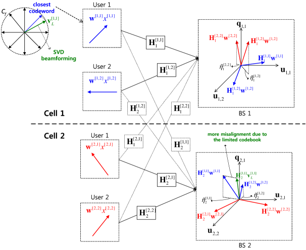
Figure 2: The codebook-based OIA where $K=2$, $M=3$, $S=2$.

Figure 2 illustrates the principle of the proposed signaling for $K=2$, $M=3$, and $S=2$. If interference $\mathbf{H}_{i}^{[k,m]}\mathbf{w}^{[k,m]}$ in (1) is perfectly aligned to the interference basis $\mathbf{Q}_{i}$, i.e., $\mathbf{H}_{i}^{[k,m]}\mathbf{w}^{[k,m]}\in\textrm{span}(\mathbf{Q}_{i})$, then interference in $\mathbf{r}_{i}$ of (4) vanishes because $\mathbf{U}_{i}^{\textrm{H}}\mathbf{H}_{i}^{[k,m]}\mathbf{w}^{[k,m]}=\mathbf{0}$. As illustrated in Fig. 2, the value $\|\mathbf{U}_{i}^{\textrm{H}}\mathbf{H}_{i}^{[k,m]}\mathbf{w}^{[k,m]}\|^{2}$ represents the amount of the signal transmitted from user $m$ in the $k$th cell to BS $i$ that is not aligned to the interference reference basis $\mathbf{Q}_{i}$. This misalignment becomes higher than the SVD-based OIA case, due to the finite codebook size.

IV Achievability Results

It was shown in [7] that using the SVD-based OIA scheme leads to a comparatively less number of users required to achieve the maximum DoF in the MIMO IMAC model. In this section, we derive the number of feedforward bits required to achieve the same achievability as the SVD-based OIA case in terms of the DoF and user scaling condition when two different types of codebook-based OIA schemes, i.e., the Grassmannian and random codebook-based OIAs, are used.

In our analysis, we use the total DoF defined as [1]

$$\textrm{DoF}=\lim_{\textrm{SNR}\rightarrow\infty}\frac{\sum_{i=1}^{K}\sum_{j=1}^{S}R^{[i,j]}}{\operatorname{log}_{2}\textrm{SNR}},$$

where $R^{[i,j]}$ is the achievable rate for user $j$ in the $i$th cell and $\textrm{SNR}=1/N_{0}$.

IV-A Grassmannian Codebook-Based OIA

We start with the following three lemmas which shall be used to establish our main theorem.

Lemma 1

For any given codebook, the LIF metric $\eta^{[i,j]}$ in (2) is upper-bounded by

$$\eta^{[i,j]}\leq{\sigma^{[i,j]}_{L}}^{2}+{d^{[i,j]}}^{2}{\sigma_{1}^{[i,j]}}^{2},$$ (6)

where $d^{[i,j]}$ is the residual distance defined by

$$d^{[i,j]}=\sqrt{1-\left|{\mathbf{w}^{[i,j]}}^{\textrm{H}}\mathbf{v}_{L}^{[i,j]}\right|^{2}}$$ (7)

and $\sigma^{[i,j]}_{m}$ is the $m$th singular value of the stacked interference channel matrix in (3).

Proof:

Since $\mathbf{v}_{L}^{[i,j]}$ is isotropically distributed over the $L$-dimensional sphere with identically and isotropically distributed (i.i.d.) complex Gaussian channel matrices [24], the weight vector $\mathbf{w}^{[i,j]}$ chosen from a codebook can be written by $\mathbf{w}^{[i,j]}=\sqrt{1-{d^{[i,j]}}^{2}}\mathbf{v}_{L}^{[i,j]}+d^{[i,j]}\mathbf{t}^{[i,j]}$ [25, 13], where $0\leq{d^{[i,j]}}^{2}\leq 1$ accounts for the quantization error and $\mathbf{t}^{[i,j]}$ is a unit-norm vector i.i.d. over $\textrm{null}\left(\mathbf{v}_{L}^{[i,j]}\right)$. Then, $\eta^{[i,j]}$ in (2) is bounded by

$$\eta^{[i,j]} =\left\|\sqrt{1-{d^{[i,j]}}^{2}}\mathbf{G}^{[i,j]}\mathbf{v}^{[i,j]}_{L}+{d^{[i,j]}}\mathbf{G}^{[i,j]}\mathbf{t}^{[i,j]}\right\|^{2}$$

$$\leq(1-{d^{[i,j]}}^{2}){\sigma^{[i,j]}_{L}}^{2}+{d^{[i,j]}}^{2}\left\|\mathbf{G}^{[i,j]}\mathbf{t}^{[i,j]}\right\|^{2}$$

$$\leq{\sigma^{[i,j]}_{L}}^{2}+{d^{[i,j]}}^{2}{\sigma_{1}^{[i,j]}}^{2},$$ (8)

where (8) follows from $\left\|\mathbf{G}^{[i,j]}\mathbf{t}^{[i,j]}\right\|^{2}\leq{\sigma_{1}^{[i,j]}}^{2}$ for any unit-norm vector $\mathbf{t}^{[i,j]}$, which proves the lemma. ∎

Now, we further bound the LIF metric for the Grassmannian codebook as follows.

Lemma 2

By using the Grassmannian codebook, $\eta^{[i,j]}$ is further bounded by $\eta^{[i,j]}\leq{\sigma^{[i,j]}_{L}}^{2}+\nu_{f}{\sigma_{1}^{[i,j]}}^{2}$, where $\nu_{f}$ denotes the number of feedforward bits given by

$$\nu_{f}=\left(\frac{1}{N_{f}}\right)^{1/(L-1)}$$ (9)

and $N_{f}$ is the number of elements in the codebook set.

Proof:

The Grassmannian codebook $\mathcal{C}_{f}$ is the set of codewords chosen by the optimal sphere packing for the $L$-dimensional sphere; namely, the chordal distance of any two codewords is all the same, i.e., $\sqrt{1-\left|{\mathbf{c}_{i}}^{\textrm{H}}\mathbf{c}_{j}\right|^{2}}=d$ for any $i\neq j$ and $d\geq 0$. Based on this property, the Rankin, Gilbert-Varshamov, and Hamming bounds on the distance of the codebook give us [26, 25]

$${d^{[i,j]}}^{2}\leq\operatornamewithlimits{min}\left\{\frac{1}{2},\frac{(L-1)N_{f}}{2L(N_{f}-1)},\left(\frac{1}{N_{f}}\right)^{1/(L-1)}\right\}.$$ (10)

For large $N_{f}$, the third term of (10) becomes dominant, thus providing an arbitrarily tight bound. Inserting (10) to (6) proves the lemma. ∎

From Lemma 2, we also have the following lemma.

Lemma 3

For the Grassmannian codebook, it follows that $\eta^{[i,j]}\leq\eta^{[i,j]}_{\textrm{GC}}$ where

$$\eta^{[i,j]}_{\textrm{GC}}=\left\{\begin{array}[]{cc}C_{1}\nu_{f}{\sigma_{1}^{[i,j]}}^{2}&\textrm{ if }{\sigma_{L}^{[i,j]}}^{2}\leq(1+\delta)\nu_{f}{\sigma_{1}^{[i,j]}}^{2}\\ C_{2}{\sigma_{L}^{[i,j]}}^{2}&\textrm{ otherwise},\end{array}\right.$$ (11)

for any constant $\delta\geq 0$ independent of SNR. Here, $C_{1}=(2+\delta)$ and $C_{2}=(1+1/(1+\delta))$; thus, $1\leq C_{2}\leq 2$.

Now we are ready to show our first main theorem, which derives the number of feedforward bits, required to achieve the same user scaling condition as the SVD-based OIA case, for the proposed OIA with Grassmannian codebook.

Theorem 1

The codebook-based OIA with the optimal Grassmannian codebook $\mathcal{C}_{f}$ [24] achieves the user scaling condition of the SVD-based OIA if 

$$n_{f}=\Omega\left(L\operatorname{log}_{2}\textrm{SNR}\right)\textrm{ bits}.$$ (12)

Moreover, under the condition (12), $KS$ DoF are achievable with high probability if $N=\omega\left(\textrm{SNR}^{(K-1)S-L+1}\right)$.

Proof:

Let us start from showing the following simple bound on $\textrm{SINR}^{[i,j]}$ in (5):

$$\textrm{SINR}^{[i,j]}\geq\frac{\textrm{SNR}/\left\|\mathbf{f}_{i,j}\right\|^{2}}{1+I^{[i,j]}},$$ (13)

where $I^{[i,j]}\triangleq\sum_{k=1,k\neq i}^{K}\sum_{m=1}^{S}\left\|{\mathbf{U}_{i}}^{\textrm{H}}\mathbf{H}_{i}^{[k,m]}\mathbf{w}^{[k,m]}\right\|^{2}\textrm{SNR}$. Suppose that $I^{[i,j]}\leq\epsilon$ for some constant $\epsilon>0$ independent of the received SNR so that each user achieves 1 DoF. By this principle, we obtain a lower bound on the achievable DoF for the codebook-based OIA as $\textrm{DoF}\geq KS\cdot\mathcal{P}$, where

$$\mathcal{P}\triangleq \lim_{\textrm{SNR}\rightarrow\infty}\textrm{Pr}\biggl{\{}I^{[i,j]}\leq\epsilon,\forall\textrm{user $j$ and BS $i$},j\in\mathcal{S}\triangleq\{1,\dots,S\},i\in\mathcal{K}\triangleq\{1,\dots,K\}\biggr{\}}.$$ (14)

From the fact that the sum of received interference at all the BSs is equivalent to the sum of the LIF metrics [4, 7], i.e.,

$$\sum_{i=1}^{K}\sum_{k=1,k\neq i}^{K}\sum_{m=1}^{S}\left\|{\mathbf{U}_{i}}^{\textrm{H}}\mathbf{H}_{i}^{[k,m]}\mathbf{w}^{[i,j]}\right\|^{2}=\sum_{i=1}^{K}\sum_{j=1}^{S}\eta^{[i,j]},$$ (15)

we can bound $\mathcal{P}$ as

$$\mathcal{P} \geq\lim_{\textrm{SNR}\rightarrow\infty}\textrm{Pr}\bigg{\{}\sum_{i=1}^{K}\sum_{j=1}^{S}I^{[i,j]}\leq\epsilon\bigg{\}}$$

$$\geq\lim_{\textrm{SNR}\rightarrow\infty}\textrm{Pr}\left\{\eta^{[i,j]}\leq\frac{\epsilon\textrm{SNR}^{-1}}{KS^{2}},\forall i\in\mathcal{K},\forall j\in\mathcal{S}\right\}.$$ (16)

At this point, let us choose $N_{f}$ such that $N_{f}^{1/(L-1)}\geq\textrm{SNR}^{(1+\gamma)}$ for $\gamma>0$, i.e.,

$$n_{f}=\operatorname{log}_{2}N_{f}\geq(1+\gamma)(L-1)\operatorname{log}_{2}\textrm{SNR},$$ (17)

resulting in (12). From (9) and (17), $\nu_{f}$ is bounded by

$$\nu_{f}=N_{f}^{-1/(L-1)}\leq\textrm{SNR}^{-(1+\gamma)}.$$ (18)

Now we consider the LIF-overestimating modification by using the upper bound $\eta^{[i,j]}_{\textrm{GC}}$ in Lemma 3. From $\eta^{[i,j]}\leq\eta^{[i,j]}_{\textrm{GC}}$ and (16), we have

$$\mathcal{P} \geq\lim_{\textrm{SNR}\rightarrow\infty}\textrm{Pr}\left\{\eta^{[i,j]}_{\textrm{GC}}\leq\frac{\epsilon\textrm{SNR}^{-1}}{KS^{2}},\forall i\in\mathcal{K},\forall j\in\mathcal{S}\right\}.$$ (19)

$$\geq\mathcal{P}_{\textrm{GC}}\triangleq\lim_{\textrm{SNR}\rightarrow\infty}\textrm{Pr}\bigg{\{}\left[\eta^{[i,j]}_{\textrm{GC}}\leq\frac{\epsilon\textrm{SNR}^{-1}}{KS^{2}},\forall i\in\mathcal{K},\forall j\in\mathcal{S}\right]$$

$$\&\left[{\sigma_{L}^{[i,j]}}^{2}\!\geq\!(1+\delta)\nu_{f}{\sigma_{1}^{[i,j]}}^{2},\forall i\in\mathcal{K},\forall j\in\mathcal{N}\triangleq\{1,\dots,N\}\right]\bigg{\}}.$$ (20)

From the principle $\textrm{Pr}(\mathcal{A}\cap\mathcal{B})=\textrm{Pr}(\mathcal{B})-\textrm{Pr}(\mathcal{A}^{c}\cap\mathcal{B})$ for sets $\mathcal{A}$ and $\mathcal{B}$, (20) can be rewritten as

$$\mathcal{P}_{\textrm{GC}}=\lim_{\textrm{SNR}\rightarrow\infty}\underbrace{\textrm{Pr}\left\{{\sigma_{L}^{[i,j]}}^{2}\geq(1+\delta)\nu_{f}{\sigma_{1}^{[i,j]}}^{2},\forall i\in\mathcal{K},\forall j\in\mathcal{N}\right\}}_{\triangleq p_{c}}$$ (21)

$$-\lim_{\textrm{SNR}\rightarrow\infty}\textrm{Pr}\bigg{\{}\biggl{[}\textrm{there exist less than $S$ users per cell such that }\eta^{[i,j]}_{\textrm{GC}}\!\leq\!\frac{\epsilon\textrm{SNR}^{-1}}{KS^{2}}\biggr{]}$$

$$~{}~{}~{}~{}~{}\&\left[{\sigma_{L}^{[i,j]}}^{2}\!\geq\!(1+\delta)\nu_{f}{\sigma_{1}^{[i,j]}}^{2},\forall i\in\mathcal{K},\forall j\in\mathcal{N}\right]\bigg{\}}\linebreak[0]$$

$$=\lim_{\textrm{SNR}\rightarrow\infty}p_{c}-\lim_{\textrm{SNR}\rightarrow\infty}\sum_{m=0}^{S-1}\left(\begin{array}[]{c}N\\ m\end{array}\right)\bigg{[}\textrm{Pr}\left\{\eta^{[i,j]}_{\textrm{GC}}\leq\frac{\epsilon\textrm{SNR}^{-1}}{KS^{2}}\hskip 3.0pt\&\hskip 5.0pt(1+\delta)\nu_{f}{\sigma_{1}^{[i,j]}}^{2}\leq{\sigma_{L}^{[i,j]}}^{2}\right\}\bigg{]}^{m}$$ (24)

$$\times\bigg{[}\underbrace{\textrm{Pr}\left\{(1+\delta)\nu_{f}{\sigma_{1}^{[i,j]}}^{2}\leq{\sigma_{L}^{[i,j]}}^{2}~{}\&~{}\frac{\epsilon\textrm{SNR}^{-1}}{C_{2}KS^{2}}\leq{\sigma_{L}^{[i,j]}}^{2}\right\}}_{\triangleq P_{o}}\bigg{]}^{N-m}$$ (25)

$$\geq\lim_{\textrm{SNR}\rightarrow\infty}p_{c}-\lim_{\textrm{SNR}\rightarrow\infty}\sum_{m=0}^{S-1}N^{m}{P_{o}}^{N-m},$$ (26)

where (25) follows from the fact that the statistics of each user is independent of each other, and (26) follows from $\textrm{Pr}\left\{\eta^{[i,j]}_{\textrm{GC}}\leq\frac{\epsilon\textrm{SNR}^{-1}}{KS^{2}}\hskip 3.0pt\&\hskip 5.0pt(1+\delta)\nu_{f}{\sigma_{1}^{[i,j]}}^{2}\leq{\sigma_{L}^{[i,j]}}^{2}\right\}\leq 1$ and $\bigg{(}\begin{array}[]{c}N\\ i\end{array}\bigg{)}=\frac{N!}{i!(N-i)!}\leq N^{i}$.

For the rest of the proof, we show that (26) tends to one under certain conditions. In Appendix A, we first show that for given $\gamma>0$ and $\delta>0$, it follows that

$$\lim_{\textrm{SNR}\rightarrow\infty}p_{c}=1,\textrm{ if $N=O\left(\textrm{SNR}^{(1+\beta)((K-1)S-L+1)}\right)$}\textrm{~{}~{}where $\beta<\gamma$.}$$

Now we show that the second term of (26) tends to zero as the SNR increases. From the fact that $\textrm{Pr}\{[A\leq B]\&[C\leq B]\}=\textrm{Pr}\{[A\leq B]|A\geq C\}\textrm{Pr}\{A\geq C\}+\textrm{Pr}\{[C\leq B]|A<C\}\textrm{Pr}\{A<C\}$ for random variables $A$, $B$, and $C$, the probability $P_{o}$ can be written as

$$P_{o}= \textrm{Pr}\biggl{\{}(1+\delta)\nu_{f}{\sigma_{1}^{[i,j]}}^{2}\leq{\sigma_{L}^{[i,j]}}^{2}\Big{|}(1+\delta)\nu_{f}{\sigma_{1}^{[i,j]}}^{2}\geq\frac{\epsilon\textrm{SNR}^{-1}}{C_{2}KS^{2}}\biggr{\}}\cdot p_{o}^{\prime}$$

$$+\textrm{Pr}\left\{\frac{\epsilon\textrm{SNR}^{-1}}{C_{2}KS^{2}}\leq{\sigma_{L}^{[i,j]}}^{2}\Big{|}(1+\delta)\nu_{f}{\sigma_{1}^{[i,j]}}^{2}<\frac{\epsilon\textrm{SNR}^{-1}}{C_{2}KS^{2}}\right\}\cdot(1-p_{o}^{\prime})$$

where $p_{o}^{\prime}=\textrm{Pr}\left\{(1+\delta)\nu_{f}{\sigma_{1}^{[i,j]}}^{2}\geq\frac{\epsilon\textrm{SNR}^{-1}}{C_{2}KS^{2}}\right\}$. From (18), for any given channel instance, we have

$$\lim_{\textrm{SNR}\rightarrow\infty}p_{o}^{\prime} \leq\lim_{\textrm{SNR}\rightarrow\infty}\textrm{Pr}\left\{(1+\delta)\textrm{SNR}^{-(1+\gamma)}{\sigma_{1}^{[i,j]}}^{2}\geq\frac{\epsilon\textrm{SNR}^{-1}}{C_{2}KS^{2}}\right\}$$

$$=\lim_{\textrm{SNR}\rightarrow\infty}\textrm{Pr}\left\{{\sigma_{1}^{[i,j]}}^{2}\geq\frac{\epsilon\textrm{SNR}^{\gamma}}{(1+\delta)C_{2}KS^{2}}\right\}=0,$$

which results in

$$\lim_{\textrm{SNR}\rightarrow\infty}P_{o} =\lim_{\textrm{SNR}\rightarrow\infty}\textrm{Pr}\left\{\frac{\epsilon\textrm{SNR}^{-1}}{C_{2}KS^{2}}\leq{\sigma_{L}^{[i,j]}}^{2}\right\}.$$

From [27, Theorem 4], we have

$$\textrm{Pr}\left\{\frac{\epsilon\textrm{SNR}^{-1}}{C_{2}KS^{2}}\leq{\sigma_{L}^{[i,j]}}^{2}\right\}$$

$$=1-\alpha\left(\frac{\epsilon}{C_{2}KS^{2}}\right)^{\psi}\textrm{SNR}^{-\psi}+o\left(\textrm{SNR}^{-\psi}\right),$$ (27)

where $\psi\triangleq(K-1)S-L+1$ and $\alpha>0$ is a constant determined by $K$, $S$, and $L$. Applying (IV-A) to (26) yields

$$\mathcal{P}\geq\mathcal{P}_{\textrm{GC}}\geq\lim_{\textrm{SNR}\rightarrow\infty}p_{c}-\lim_{\textrm{SNR}\rightarrow\infty}\sum_{i=0}^{S-1}N^{m}\Biggl{[}1-\alpha\left(\frac{\epsilon}{C_{2}KS^{2}}\right)^{\psi}\textrm{SNR}^{-\psi}\hskip 15.0pt+o\left(\textrm{SNR}^{-\psi}\right)\Biggr{]}^{N-m}.$$ (28)

For given $\gamma$ and $0<\beta<\gamma$, let us choose $N=O\left(\textrm{SNR}^{(1+\beta)((K-1)S-L+1)}\right)$. Then, from (IV-A), it follows that $\lim_{\textrm{SNR}\rightarrow\infty}p_{c}=1$. On the other hand, the second term of (28) tends to zero because $N^{m}$ increases polynomially with SNR for given $m$ while $\left[1-\alpha\left(\frac{\epsilon}{C_{2}KS^{2}}\right)^{\psi}\textrm{SNR}^{-\psi}+o\left(\textrm{SNR}^{-\psi}\right)\right]^{N-m}$ decreases exponentially with SNR. Thus, $\mathcal{P}$ tends to one, which means that $KS$ DoF are achievable.

As assumed earlier, note that our analysis holds for $\beta<\gamma$. However, it is obvious that assuming either the condition $N=O\left(\textrm{SNR}^{(1+\beta)((K-1)S-L+1)}\right)$ for any $\beta\geq\gamma$ or $N=\omega\left(\textrm{SNR}^{(K-1)S-L+1}\right)$ leads to the same or higher DoF compared to the case for $0\leq\beta<\gamma$, due to the fact that increasing $N$ for given $n_{f}$ and SNR values yields a reduced LIF and thus an increased achievable rate for all the selected users. Since the maximum achievable DoF are upper-bounded by $KS$ for given $S$, the last argument indicates that $KS$ DoF are achievable if $n_{f}=\Omega(L\operatorname{log}_{2}\textrm{SNR})$ and $N=\omega\left(\textrm{SNR}^{(K-1)S-L+1}\right)$, which completes the proof. ∎

Theorem 1 indicates that $n_{f}$ should scale with SNR so as to achieve the target DoF under the same user scaling condition as the SVD-based OIA case, and that from (17), no more feedforward bits than $(1+\gamma)(L-1)\operatorname{log}_{2}\textrm{SNR}$ are indeed required. The derived $n_{f}$ scaling condition is proportional to $L$ and $\operatorname{log}_{2}\textrm{SNR}$, which is consistent with the previous results on the number of feedback bits required to avoid performance loss due to the finite codebook size in a variety of limited feedback systems [24, 13, 9].

IV-B Random Codebook-Based OIA

For a random codebook scenario, each element $\mathbf{c}_{n}$ of $\mathcal{C}_{f}$ ($n\in\{1,\ldots,N_{f}\}$) is chosen independently and isotropically from the $L$-dimensional sphere. The following second main theorem shows that the same user scaling condition as the Grassmannian codebook-based OIA case is obtained even with the random codebook-based OIA.

Theorem 2

The codebook-based OIA with a random codebook achieves $KS$ DoF with high probability if $N=\omega\left(\textrm{SNR}^{(K-1)S-L+1}\right)$ and $n_{f}=\Omega\left(L\operatorname{log}_{2}\textrm{SNR}\right)$ bits.

Proof:

Since equations (13)–(16) also hold for the random codebook approach, we only show that $\mathcal{P}$ in (14) tends to one under two conditions $N=\omega\left(\textrm{SNR}^{(K-1)S-L+1}\right)$ and $n_{f}=\Omega\left(L\operatorname{log}_{2}\textrm{SNR}\right)$. Unlike the Grassmannian codebook, the residual distance $d^{[i,j]}$ in (7) is now a random variable and thus is unbounded. Note that the cumulative density function (CDF) of the squared chordal distance between any two independent unit random vectors chosen isotropically from the $L$-dimensional sphere is given by $\beta(L-1,1)$, where $\beta(x,y)=\int_{0}^{1}t^{x-1}(1-t)^{y-1}dt$ is the beta function [13]. Since ${d^{[i,j]}}^{2}$ for the random codebook is the minimum of $N_{f}$ independent random variables with distribution $\beta(L-1,1)$, the CDF of ${d^{[i,j]}}^{2}$ is given by

$$\textrm{Pr}\left\{{d^{[i,j]}}^{2}\leq z\right\}=1-\left(1-z^{L-1}\right)^{N_{f}}.$$ (29)

Now, let us again consider the following modification for given channel instance:

• if ${d^{[i,j]}}^{2}\leq\textrm{SNR}^{-(1+\gamma)}$ for all $i$ and $j$, then the same LIF-overestimating modification as the Grassmannian codebook case is used, where the LIF values are replaced with their upper bounds. Specifically, from Lemma 1, we shall use the following upper bound on $\eta^{[i,j]}$:

  $$\eta^{[i,j]}_{\textrm{RC}}\!\!=\!\!\left\{\begin{array}[]{cc}\!\!\!C_{3}{d^{[i,j]}}^{2}{\sigma_{1}^{[i,j]}}^{2}&\textrm{if~{}}{\sigma_{L}^{[i,j]}}^{2}\!\!\leq\!\!(1+\delta^{\prime}){d^{[i,j]}}^{2}{\sigma_{1}^{[i,j]}}^{2}\\ \!\!\!C_{4}{\sigma_{L}^{[i,j]}}^{2}&\textrm{otherwise},\end{array}\right.$$ (30)

  for any constant $\delta^{\prime}\geq 0$ independent of SNR, where $C_{3}=(2+\delta^{\prime})$ and $C_{4}=(1+1/(1+\delta^{\prime}))$; thus, $1\leq C_{4}\leq 2$,

• otherwise, i.e., if ${d^{[i,j]}}^{2}>\textrm{SNR}^{-(1+\gamma)}$ for any $i$ or $j$, then we drop the case by assuming 0 DoF for this case.

Let us define the event $\mathcal{D}$ as

$$\mathcal{D} =\bigl{\{}{d^{[i,j]}}^{2}\leq\textrm{SNR}^{-(1+\gamma)},\forall i\in\mathcal{K}=\{1,\dots,K\},\forall j\in\mathcal{N}=\{1,\dots,N\}\bigr{\}}.$$

From $\eta^{[i,j]}\leq\eta^{[i,j]}_{\textrm{RC}}$, we have

$$\mathcal{P} \geq\lim_{\textrm{SNR}\rightarrow\infty}\textrm{Pr}\biggl{\{}\eta^{[i,j]}\leq\frac{\epsilon\textrm{SNR}^{-1}}{KS^{2}},\forall i\in\mathcal{K},\forall j\in\mathcal{S}=\{1,\dots,S\}\biggr{\}}$$

$$\geq\mathcal{P}_{\textrm{RC}}\triangleq\lim_{\textrm{SNR}\rightarrow\infty}\textrm{Pr}\left\{\mathcal{D}\right\}\cdot\textrm{Pr}\left\{\eta^{[i,j]}_{\textrm{RC}}\leq\frac{\epsilon\textrm{SNR}^{-1}}{KS^{2}},\forall i\in\mathcal{K},\forall j\in\mathcal{S}\bigg{|}\mathcal{D}\right\}.$$

From (29) and the inequality $(1-x)^{y}>1-xy$ for any $0<x<1<y$, we have

$$\textrm{Pr}\left\{\mathcal{D}\right\} =\left(1-\left(1-\left(\textrm{SNR}^{-(1+\gamma)}\right)^{L-1}\right)^{N_{f}}\right)^{KN}$$

$$>1-KN\left(1-\textrm{SNR}^{-(1+\gamma)(L-1)}\right)^{N_{f}}.$$ (31)

Let us choose $N$ such that $N$ scales polynomially with SNR. If $N_{f}$ scales faster than $\textrm{SNR}^{(1+\gamma)(L-1)}$, then the second term of (31) vanishes as the SNR increases, because $\left(1-\textrm{SNR}^{-(1+\gamma)(L-1)}\right)^{N_{f}}$ decreases exponentially with SNR while $N$ increases polynomially with SNR.

Now recall that for the Grassmannian codebook approach, ${d^{[i,j]}}^{2}$ is bounded by ${d^{[i,j]}}^{2}\leq\nu_{f}\leq\textrm{SNR}^{-(1+\gamma)}$ along with the choice of $n_{f}\geq(1+\gamma)(L-1)\operatorname{log}_{2}\textrm{SNR}$, and that our achievability proof is based on the upper bound on the LIF metric in (11). If $\mathcal{D}$ holds, then the upper bound in (30) is identical to (11), and thus it is not difficult to show that if $N=O\left(\textrm{SNR}^{(1+\beta)((K-1)S-L+1)}\right)$ for any $0<\beta<\gamma$, then

$$\lim_{\textrm{SNR}\rightarrow\infty}\textrm{Pr}\left\{\eta^{[i,j]}_{\textrm{RC}}\leq\frac{\epsilon\textrm{SNR}^{-1}}{KS^{2}},\forall i\in\mathcal{K},\forall j\in\mathcal{S}\bigg{|}\mathcal{D}\right\}=1,$$ (32)

as shown in (19)–(28). From (31) and (32), choosing the two conditions $n_{f}=\operatorname{log}_{2}N_{f}\geq(1+\gamma)(L-1)\operatorname{log}_{2}\left(\textrm{SNR}\right)$, i.e., $n_{f}=\Omega(L\operatorname{log}_{2}(\textrm{SNR}))$, and $N=O\left(\textrm{SNR}^{(1+\beta)((K-1)S-L+1)}\right)$ for any $0<\beta<\gamma$, the probability $\mathcal{P}_{\textrm{RC}}$ tends to one for increasing SNR. Note that taking the limit of $N$ polynomially increasing with SNR comes merely from the strict condition of $\mathcal{D}$. Since increasing $N$ for given $n_{f}$ lowers the LIF and thereby increases the achievable rate for each selected user, $\mathcal{P}$ tends to one for any $N=\omega\left(\textrm{SNR}^{(K-1)S-L+1}\right)$, which completes the proof. ∎

Interestingly, Theorem 2 indicates that the required $n_{f}$ for the random codebook is the same as that for the Grassmannian codebook. This is an encouraging result since analytical construction methods of the Grassmannian codebook for large $n_{f}$ have been unknown, and even its numerical construction requires excessive computational complexity. We complete the achievability discussion by providing the following remarks.

Remark 1 (Random vs. Grassmannian codebook)

In the previous work on limited feedback systems, the performance analysis has focused on the average SNR or the average rate loss [28]. It has been known that the Grassmannian codebook outperforms the random codebook in the average sense. However, in our OIA framework, the focus is on the asymptotic performance for increasing SNR, and it turns out that the asymptotic behavior is the same for the two codebook approaches. In fact, our result is consistent with the previous work on limited feedback systems (see [29]), where the performance gap between two codebooks was shown to be negligible as the number of feedback bits increases.

Remark 2 (Comparison to the MIMO broadcasting channel)

For the MIMO broadcasting channel with limited feedback, where the transmitter has $L$ antennas employing the random codebook, it was shown in [13] that the achievable rate loss for each user, denoted by $\Delta R$, coming from the finite size of the codebook is given by $\Delta<\operatorname{log}_{2}\left(1+\textrm{SNR}\cdot 2^{-n_{f}/(L-1)}\right)$. Thus, to achieve the maximum DoF for each user, or to make the rate loss negligible as the SNR increases, the term $\textrm{SNR}\cdot 2^{-n_{f}/(L-1)}$ should remain constant for increasing SNR. That is, $n_{f}$ should scale faster than $(L-1)\operatorname{log}_{2}\textrm{SNR}$. Although the system model and signaling methodology under consideration are different from our setting, Theorems 1 and 2 are consistent with this previous result.

V Asymptotically Optimal Receiver Design at the BSs

While using the ZF receiver is sufficient to achieve the maximum DoF, we study the design of an enhanced receiver at the BSs in pursuit of improving the achievable rate. Recall that each BS is not assumed to have CSI of the cross-links from the users in the other cells, because no coordination between BSs is assumed. In this section, the main challenge is thus to decode the desired symbols with no CSI of the cross-links at the receivers. For convenience, let us rewrite the received signal at BS $i$ in (1) as

$$\mathbf{y}_{i} =\tilde{\mathbf{H}}_{i}^{(c)}\mathbf{x}_{i}+\sum_{k=1,k\neq i}^{K}\sum_{m=1}^{S}\mathbf{H}_{i}^{[k,m]}\mathbf{w}^{[k,m]}x^{[k,m]}+\mathbf{z}_{i},$$ (33)

where $\tilde{\mathbf{H}}_{i}^{(c)}\triangleq\left[\mathbf{H}_{i}^{[i,1]}\mathbf{w}^{[i,1]},\ldots\mathbf{H}_{i}^{[i,S]}\mathbf{w}^{[i,S]}\right]\in\mathbb{C}^{M\times S}$ and $\mathbf{x}_{i}\triangleq\left[x^{[i,1]},\ldots,x^{[i,S]}\right]^{\textrm{T}}\in\mathbb{C}^{S\times 1}$. The channel capacity $I_{\textrm{C}}$ is given by [30]

$$I_{\textrm{C}}=\operatorname{log}_{2}\det\left(\mathbf{R}_{c}^{-1/2}\tilde{\mathbf{H}}_{i}^{(c)}\left(\tilde{\mathbf{H}}_{i}^{(c)}\right)^{\textrm{H}}\mathbf{R}_{c}^{-1/2}+\mathbf{I}_{M}\right),$$ (34)

where

$$\mathbf{R}_{c}=\sum_{k=1,k\neq i}^{K}\sum_{m=1}^{S}\mathbf{H}_{i}^{[k,m]}\mathbf{w}^{[k,m]}\left(\mathbf{H}_{i}^{[k,m]}\mathbf{w}^{[k,m]}\right)^{\textrm{H}}+N_{0}\mathbf{I}_{M},$$ (35)

which is not available at BS $i$ due to the assumption of unknown inter-cell interfering links. The channel capacity $I_{\textrm{C}}$ is achievable with the optimal ML decoder

$$\hat{\mathbf{x}}_{i}^{\textrm{ML}}=\underset{\mathbf{x}}{\operatorname{arg}\operatornamewithlimits{min}}\left(\mathbf{y}_{i}-\tilde{\mathbf{H}}_{i}^{(c)}\mathbf{x}\right)^{\textrm{H}}\mathbf{R}_{c}^{-1}\left(\mathbf{y}_{i}-\tilde{\mathbf{H}}_{i}^{(c)}\mathbf{x}\right),$$ (36)

which is infeasible to implement due to unknown $\mathbf{R}_{c}$. After nulling interference by multiplying $\mathbf{U}_{i}$, the received signal is given by

$$\tilde{\mathbf{y}}_{i} =\mathbf{U}_{i}^{\textrm{H}}\mathbf{y}_{i}=\tilde{\mathbf{H}}_{i}\mathbf{x}_{i}+\underbrace{\sum_{k=1,k\neq i}^{K}\sum_{m=1}^{S}\mathbf{U}_{i}^{\textrm{H}}\mathbf{H}_{i}^{[k,m]}\mathbf{w}^{[k,m]}x^{[k,m]}+\mathbf{U}_{i}^{\textrm{H}}\mathbf{z}_{i}}_{\tilde{\mathbf{z}}_{i}},$$ (37)

where $\tilde{\mathbf{H}}_{i}\triangleq\left[\mathbf{U}_{i}^{\textrm{H}}\mathbf{H}_{i}^{[i,1]}\mathbf{w}^{[i,1]},\ldots\mathbf{U}_{i}^{\textrm{H}}\mathbf{H}_{i}^{[i,S]}\mathbf{w}^{[i,S]}\right]\in\mathbb{C}^{S\times S}$ and $\tilde{\mathbf{z}}_{i}\in\mathbb{C}^{S\times 1}$ represents the effective noise. Let us denote the covariance matrix of the effective noise after interference nulling by

$$\mathbf{R} \triangleq E\left\{\tilde{\mathbf{z}_{i}}\tilde{\mathbf{z}_{i}}^{\textrm{H}}\right\}$$

$$=\sum_{k=1,k\neq i}^{K}\sum_{m=1}^{S}\mathbf{U}_{i}^{\textrm{H}}\mathbf{H}_{i}^{[k,m]}\mathbf{w}^{[k,m]}\left(\mathbf{U}_{i}^{\textrm{H}}\mathbf{H}_{i}^{[k,m]}\mathbf{w}^{[k,m]}\right)^{\textrm{H}}+N_{0}\mathbf{I}_{S}.$$ (38)

Then, the ML decoder for the modified channel (37) becomes ${\operatorname{arg}\operatornamewithlimits{min}}_{\mathbf{x}}\left(\tilde{\mathbf{y}}_{i}-\tilde{\mathbf{H}}_{i}\mathbf{x}\right)^{\textrm{H}}\mathbf{R}^{-1}\left(\tilde{\mathbf{y}}_{i}-\tilde{\mathbf{H}}_{i}\mathbf{x}\right)$, which is also infeasible to implement since the term $\mathbf{U}_{i}^{\textrm{H}}\mathbf{H}_{i}^{[k,m]}\mathbf{w}^{[k,m]}$ ($k\in\{1,\ldots,i-1,i+1,\ldots,K\}$, $m\in\{1,\ldots,S\}$) is not available at BS $i$.

As an alternative approach, we now introduce the following minimum Euclidean distance receiver after interference nulling at BS $i$:

$$\hat{\mathbf{x}}_{i}=\operatorname{arg}_{\mathbf{x}}\operatornamewithlimits{min}\left\|\tilde{\mathbf{y}}_{i}-\tilde{\mathbf{H}}_{i}\mathbf{x}\right\|.$$ (39)

It is worth noting that the receiver in (39) is not universally optimal since $\mathbf{R}$ is not an identity matrix for given channel instance. Now, we show the achievable rate based on the use of the receiver in (39). The maximum achievable rate of any suboptimal receiver, referred to as mismatch capacity [31, 32], is lower-bounded by the generalized mutual information, defined as [31, 32]

$$I_{\textrm{GMI}}=\sup_{\theta\geq 0}I(\theta),$$ (40)

where

$$I(\theta)\triangleq E\left[\operatorname{log}_{2}\frac{Q(\tilde{\mathbf{y}}_{i}|\mathbf{x}_{i})^{\theta}}{E\left[Q(\tilde{\mathbf{y}}_{i}|\mathbf{x}_{i})^{\theta}\big{|}\tilde{\mathbf{y}}_{i},\tilde{\mathbf{H}}_{i}\right]}\bigg{|}\tilde{\mathbf{H}}_{i}\right]$$ (41)

and $Q(\tilde{\mathbf{y}}_{i}|\mathbf{x}_{i})$ is the decoding metric expressed in probability. The following lemma characterizes the GMI of the decoder with mismatched noise covariance matrix.

Lemma 4

Consider the modified channel (37) and the decoding metric with mismatched noise covariance matrix $\hat{\mathbf{R}}$, given by

$$Q(\tilde{\mathbf{y}}_{i}|\mathbf{x}_{i})=\operatorname{exp}\left(-(\tilde{\mathbf{y}}_{i}-\tilde{\mathbf{H}}_{i}\mathbf{x}_{i})^{\textrm{H}}\hat{\mathbf{R}}^{-1}(\tilde{\mathbf{y}}_{i}-\tilde{\mathbf{H}}_{i}\mathbf{x}_{i})\right).$$ (42)

Then, the GMI $I_{\textrm{GMI}}$ based on the metric (42) is given by (40), where $I(\theta)$ for given $\hat{\mathbf{R}}$ is expressed as

$$I(\theta)=-\frac{\theta}{\operatorname{log}2}\textrm{tr}(\hat{\mathbf{R}}^{-1/2}\mathbf{R}\hat{\mathbf{R}}^{-1/2})+\frac{\theta}{\operatorname{log}2}\left[\textrm{tr}\left(\boldsymbol{\Omega}^{-1}\hat{\mathbf{R}}^{-1}\left(\tilde{\mathbf{H}}_{i}\tilde{\mathbf{H}}_{i}^{\textrm{H}}+\mathbf{R}\right)\right)\right]+\operatorname{log}_{2}\det(\boldsymbol{\Omega}),$$ (43)

$\mathbf{R}$ is given by (V), and $\boldsymbol{\Omega}\triangleq\theta\hat{\mathbf{R}}^{-1}\tilde{\mathbf{H}}_{i}\tilde{\mathbf{H}}_{i}^{\textrm{H}}+\mathbf{I}_{S}$.

Proof:

See Appendix B. ∎

We remark that if $\mathbf{R}=\hat{\mathbf{R}}$, then it is obvious to show $I_{\textrm{GMI}}=I(\theta=1)$. In this case, using (43), $I(\theta=1)$ can be simplified to $I(\theta=1)=\operatorname{log}_{2}\det(\mathbf{R}^{-1}\tilde{\mathbf{H}}_{i}\tilde{\mathbf{H}}_{i}^{\textrm{H}}+\mathbf{I}_{S})$, which is equal to the channel capacity. The following theorem characterizes the achievable rate of the proposed minimum Euclidean distance decoder.

Theorem 3 (Asymptotic capacity)

The GMI $I_{\textrm{GMI}}$ of the codebook-based OIA using the minimum Euclidean distance receiver in (39) is given by

$$I_{\textrm{GMI}}=\sup_{\theta\geq 0}-\frac{\theta}{\operatorname{log}2}\textrm{tr}(N_{0}^{-1}\mathbf{R})+\frac{\theta}{\operatorname{log}2}\left[\textrm{tr}\left(N_{0}^{-1}{\boldsymbol{\Omega}^{\prime}}^{-1}\left(\tilde{\mathbf{H}}_{i}\tilde{\mathbf{H}}_{i}^{\textrm{H}}+\mathbf{R}\right)\right)\right]+\operatorname{log}_{2}\det(\boldsymbol{\Omega}^{\prime}),$$ (44)

which asymptotically achieves the channel capacity $I_{\textrm{C}}$ if $N=\omega\left(\textrm{SNR}^{(K-1)S-L+1}\right)$ and $n_{f}=\Omega\left(L\operatorname{log}_{2}(\textrm{SNR})\right)$, where $\boldsymbol{\Omega}^{\prime}=\theta N_{0}^{-1}\tilde{\mathbf{H}}_{i}\tilde{\mathbf{H}}_{i}^{\textrm{H}}+\mathbf{I}_{S}$.

Proof:

The decoder in (39) is equivalent to the one that utilizes the decoding metric $Q(\tilde{\mathbf{y}}_{i}|\mathbf{x}_{i})$ in (42) with $\hat{\mathbf{R}}=N_{0}\mathbf{I}_{S}$. From Lemma 4, the GMI based the minimum Euclidean distance decoder is thus given by (44).

Now, we show that as $N$ increases, $I_{\textrm{GMI}}$ approaches $I_{\textrm{C}}$ with increasing SNR. Recall that the user selection and weight vector design are performed such that interference is aligned to the reference basis matrix $\mathbf{Q}_{i}\in\mathbb{C}^{M\times(M-S)}$ as much as possible. From Theorem 1 and 2, if $N=\omega\left(\textrm{SNR}^{(K-1)S-L+1}\right)$ and $n_{f}=\Omega\left(L\operatorname{log}_{2}(\textrm{SNR})\right)$, then the sum of received interference aligned to $\mathbf{U}_{i}$ can be made arbitrarily small with high probability, thereby resulting in

$$\mathbf{H}_{i}^{[k,m]}\mathbf{w}^{[k,m]}\in\textrm{span}(\mathbf{Q}_{i})$$ (45)

from the fact that the interference term of (33) is given by $\sum_{k=1,k\neq i}^{K}\sum_{m=1}^{S}\mathbf{H}_{i}^{[k,m]}\mathbf{w}^{[k,m]}x^{[k,m]}$. Since $\mathbf{U}_{i}^{\textrm{H}}\mathbf{H}_{i}^{[k,m]}\mathbf{w}^{[k,m]}=0$, the interference term of (37) is canceled out, and thus it follows that $\mathbf{R}\rightarrow\hat{\mathbf{R}}=N_{0}\mathbf{I}_{S}$. In this case, we have

$$I_{\textrm{GMI}}\rightarrow I_{\textrm{GMI}}^{*}=\operatorname{log}_{2}\det\left(N_{0}^{-1}\tilde{\mathbf{H}}_{i}\tilde{\mathbf{H}}_{i}^{\textrm{H}}+\mathbf{I}_{S}\right).$$ (46)

Now we prove that $I_{\textrm{GMI}}^{*}$ in (46) asymptotically achieves $I_{\textrm{C}}$. Since $[\mathbf{U}_{i},\mathbf{Q}_{i}]\in\mathbb{C}^{M\times M}$ is an orthogonal matrix, $I_{\textrm{GMI}}^{*}$ can be rewritten as

$$I_{\textrm{GMI}}^{*} =\operatorname{log}_{2}\det\left(N_{0}^{-1}\mathbf{U}_{i}^{\textrm{H}}\tilde{\mathbf{H}}_{i}^{(c)}\left(\tilde{\mathbf{H}}_{i}^{(c)}\right)^{\textrm{H}}\mathbf{U}_{i}+\mathbf{I}_{S}\right),$$

$$=\operatorname{log}_{2}\det\left(\left[\begin{array}[]{cc}{N_{0}}^{-1}\mathbf{U}_{i}^{\textrm{H}}\tilde{\mathbf{H}}_{i}^{(c)}\left(\tilde{\mathbf{H}}_{i}^{(c)}\right)^{\textrm{H}}\mathbf{U}_{i}&\mathbf{0}\\ \mathbf{0}&\mathbf{0}\\ \end{array}\right]\!+\!\mathbf{I}_{M}\!\right)$$

$$=\operatorname{log}_{2}\det\Biggl{(}[\mathbf{U}_{i},\mathbf{Q}_{i}]\cdot\left[\begin{array}[]{cc}{N_{0}}^{-1}\mathbf{U}_{i}^{\textrm{H}}\tilde{\mathbf{H}}_{i}^{(c)}\left(\tilde{\mathbf{H}}_{i}^{(c)}\right)^{\textrm{H}}\mathbf{U}_{i}&\mathbf{0}\\ \mathbf{0}&\mathbf{0}\\ \end{array}\right]\cdot[\mathbf{U}_{i},\mathbf{Q}_{i}]^{\textrm{H}}+\mathbf{I}_{M}\Biggr{)}$$

$$=\operatorname{log}_{2}\det\left(\mathbf{D}\tilde{\mathbf{H}}_{i}^{(c)}\left(\tilde{\mathbf{H}}_{i}^{(c)}\right)^{\textrm{H}}\mathbf{D}+\mathbf{I}_{M}\right),$$ (48)

where

$$\mathbf{D} =[\mathbf{U}_{i},\mathbf{Q}_{i}]\left[\begin{array}[]{cc}N_{0}^{-1/2}\mathbf{I}_{S}&\mathbf{0}\\ \mathbf{0}&\mathbf{0}\end{array}\right][\mathbf{U}_{i},\mathbf{Q}_{i}]^{\textrm{H}}=N_{0}^{-1/2}\mathbf{U}_{i}{\mathbf{U}_{i}}^{\textrm{H}}.$$ (51)

From the fact that from (45), $\mathbf{H}_{i}^{[k,m]}\mathbf{w}^{[k,m]}$ can be represented as a linear combination of $\mathbf{q}_{i,1},\ldots,\mathbf{q}_{i,M-S}$, $\mathbf{R}_{c}$ in (35) is written as

$$\mathbf{R}_{c} =\sum_{k=1,k\neq i}^{K}\sum_{m=1}^{S}\sum_{l=1}^{M-S}\sum_{t=1}^{M-S}\tilde{\xi}^{[k,m]}_{l,t}\mathbf{q}_{i,l}\mathbf{q}_{i,t}^{\textrm{H}}+N_{0}\mathbf{I}_{M}$$

$$=\sum_{l=1}^{M-S}\sum_{t=1}^{M-S}\xi_{l,t}\mathbf{q}_{i,l}\mathbf{q}_{i,t}^{\textrm{H}}+N_{0}\mathbf{I}_{M}$$

$$=\sum_{l=1}^{M-S}\sum_{t=1}^{M-S}\xi_{l,t}\mathbf{q}_{i,l}\mathbf{q}_{i,t}^{\textrm{H}}+N_{0}[\mathbf{Q}_{i},\mathbf{U}_{i}]\cdot[\mathbf{Q}_{i},\mathbf{U}_{i}]^{\textrm{H}}$$

$$=[\mathbf{Q}_{i},\mathbf{U}_{i}]\cdot\left[\begin{array}[]{cc}\boldsymbol{\Xi}&\mathbf{0}\\ \mathbf{0}&N_{0}\mathbf{I}_{S}\\ \end{array}\right]\cdot[\mathbf{Q}_{i},\mathbf{U}_{i}]^{\textrm{H}},$$ (54)

where $\tilde{\xi}^{[k,m]}_{l,t}$ denotes the component coefficient of $\mathbf{H}^{[k,m]}_{i}\mathbf{w}^{[k,m]}$ on $\mathbf{q}_{i,l}\mathbf{q}_{i,t}^{\textrm{H}}$, $\xi_{l,t}=\sum_{k=1,k\neq i}^{K}\sum_{m=1}^{S}\tilde{\xi}^{[k,m]}_{l,t}$, and

$$\boldsymbol{\Xi}=\left[\begin{array}[]{cccc}\xi_{1,1}+N_{0}&\xi_{1,2}&\cdots&\xi_{1,M-S}\\ \xi_{2,1}&\xi_{2,2}+N_{0}&\cdots&\xi_{2,M-S}\\ \vdots&\ddots&\vdots&\vdots\\ \xi_{M-S,1}&\xi_{M-S,2}&\cdots&\xi_{M-S,M-S}+N_{0}\end{array}\right].$$

Since each coefficient $\xi_{l,t}$ is chosen from a continuous distribution, $\boldsymbol{\Xi}$ has full rank almost surely, and thus is invertible. Therefore, we get

$$\mathbf{R}_{c}^{-1/2}=[\mathbf{Q}_{i},\mathbf{U}_{i}]\left[\begin{array}[]{cc}\boldsymbol{\Xi}^{-1/2}&\mathbf{0}\\ \mathbf{0}&{N_{0}}^{-1/2}\mathbf{I}_{S}\\ \end{array}\right][\mathbf{Q}_{i},\mathbf{U}_{i}]^{\textrm{H}}.$$

For given channel instance, as $N_{0}$ decreases, $\mathbf{R}_{c}^{-1/2}$ becomes

$$\mathbf{R}_{c}^{-1/2}\rightarrow{N_{0}}^{-1/2}\mathbf{U}_{i}{\mathbf{U}_{i}}^{\textrm{H}}.$$ (55)

Applying the asymptotic $\mathbf{R}_{c}^{-1/2}$ of (55) to (34) finally yields $I_{\textrm{C}}$, which is equal to $I_{\textrm{GMI}}^{*}$ of (48). This completes the proof. ∎

As shown in Theorem 3, the minimum Euclidean distance receiver asymptotically achieves the channel capacity even without any coordination between the BSs or users. However, it is worth noting that if the interference alignment level is too low due to small $N$ or $n_{f}$ to satisfy the conditions in Theorems 1 and 2, then the achievable rate in (44) may be lower than that based on the ZF receiver. Thus, in small $N$ and $n_{f}$ regimes, there may exist crossovers, where the achievable rate of the two schemes is switched, which will be shown in Section VI via numerical evaluation. We conclude our discussion on the receiver design with the following remark.

Remark 3 (DoF achievability of the optimal receiver)

Even with the use of the ML receiver in (36) based on full knowledge of $\mathbf{R}_{c}$, the user and $n_{f}$ scaling conditions to achieve $KS$ DoF are the same as those based of the ZF receiver case, which make the amount of interference bounded even for increasing SNR.

VI Numerical Results

In this section, we run computer simulations to verify the performance of the proposed two types of codebook-based OIA schemes, i.e., the Grassmannian and random codebook-based OIAs, for finite system parameters SNR, $N$, and $n_{f}$. For comparison, the max-SNR scheme was used, in which each user employs eigen-beamforming in terms of maximizing its received SNR and the belonging BS selects the $S$ users who have the SNR values up to the $S$th largest one. The SVD-based OIA scheme in [7] is also compared as a baseline method.

Figures 3 show a log-log plot of the sum-LIF (or equivalently, the sum of generating interference) versus $N$ for the MIMO IMAC with $K=2$, $M=3$, $L=2$, and (a) $S=2$ or (b) $S=3$. From Theorems 1 and 2, the system parameter $S$ governs the trade-off between the achievable DoF and the number of users required to guarantee such DoF [4, 7]. It is seen that the sum-LIF increases as $S$ grows for any given scheme. However, as addressed in[4, 7], note that a smaller LIF does not necessarily leads to a higher achievable rate, especially in the high SNR regime. In addition, the trade-off between $n_{f}$ and the sum-LIF is clearly seen from Fig. 3. Although the sum-LIF level of the codebook-based OIA scheme decreases as $n_{f}$ increases, its decreasing rate of the sum-LIF with respect to $N$, representing the slope of the sum-LIF curve, slightly differs from that of the SVD-based OIA unless $n_{f}$ increases according to increasing $N$.

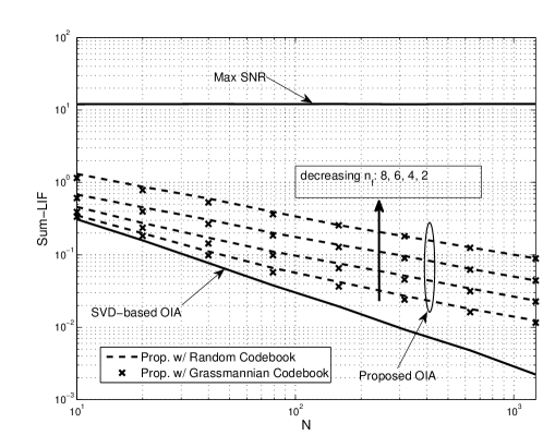
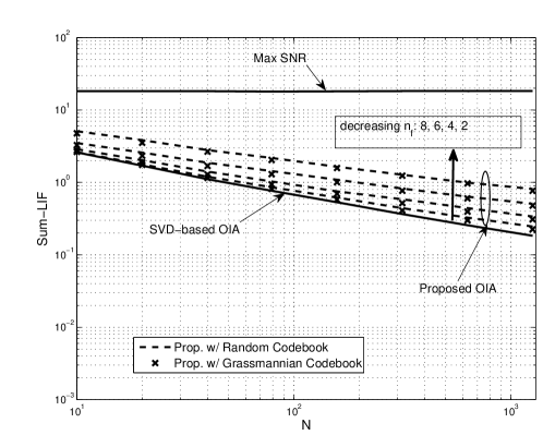
Figure 3: The sum-LIF versus $N$ when $K=2$, $M=3$, and $L=2$. (a) $S=2$. (b) $S=3$.

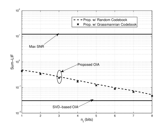
Figure 4: The sum-LIF versus $n_{f}$ when $K=2$, $M=3$, $L=2$, $S=2$, and $N=100$.

Figure 4 illustrates a linear-log plot of the sum-LIF versus $n_{f}$ when $K=2$, $M=3$, $L=2$, $S=2$ and $N=100$. As expected from Theorems 1 and 2, it is seen that the decreasing rate of the sum-LIF is almost the same for both codebook-based OIA schemes. As $n_{f}$ increases, even with finite $N$, the sum-LIF level for both codebook-based OIA schemes becomes close to that for the SVD-based OIA.

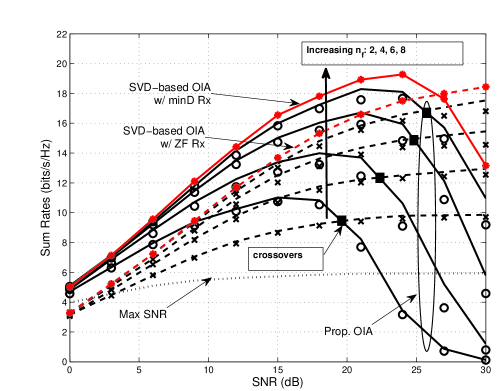
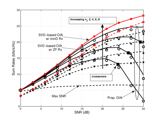
Figure 5: The achievable rate versus SNR when $K=2$, $M=3$, $L=2$, and $S=2$. (a) $N=20$. (b) $N=100$.

Figures 5 depicts the achievable rate versus SNR when $K=2$, $M=3$, $L=2$, $S=2$, and (a) $N=20$ or (b) $N=100$. We consider the following four receiver structures for the proposed codebook-based OIA:

• Scheme 1: ZF receiver with the Grassmannian codebook (dashed line)

• Scheme 2: ZF receiver with the random codebook (x)

• Scheme 3: minimum Euclidean distance receiver with the Grassmannian codebook (solid line)

• Scheme 4: minimum Euclidean distance receiver with the random codebook (o)

A relationship between the sum-rate for given $N$ and the number of feedforward bits, $n_{f}$, is observed. It is first seen that as $n_{f}=8$, the proposed codebook-based OIA schemes closely obtain the achievable rate of the SVD-based OIA. It is also seen that the gain coming from the Grassmannian codebook over the the random codebook is marginal. From Theorem 3, we remark that the achievable rate based on the minimum Euclidean distance receiver asymptotically achieves the channel capacity if interference $\mathbf{H}_{i}^{[k,m]}\mathbf{w}^{[k,m]}$ is perfectly aligned to $\mathbf{Q}_{i}$ at BS $i$; that is, the covariance matrix of interference in (V), $\sum_{k=1,k\neq i}^{K}\sum_{m=1}^{S}\mathbf{U}_{i}^{\textrm{H}}\mathbf{H}_{i}^{[k,m]}\mathbf{w}^{[k,m]}\left(\mathbf{U}_{i}^{\textrm{H}}\mathbf{H}_{i}^{[k,m]}\mathbf{w}^{[k,m]}\right)^{\textrm{H}}$, becomes negligible compared to $N_{0}\mathbf{I}_{S}$ due to the fact that interference is sufficiently aligned for large $N$. In addition, it is observed that in the low to mid SNR regimes, using the minimum Euclidean distance receiver leads to a higher sum rate than the ZF receiver case even for practical $N$. However, as the SNR increases beyond a certain point, i.e., in the high SNR regime, the covariance matrix of interference becomes dominant, thus yielding a performance degradation of the minimum Euclidean distance receiver. On the other hand, since the ZF receiver has no such limitation, its achievable rate increases with SNR. In consequence, for given $N$, there exist crossovers, where the achievable rate of the two schemes is switched. It is furthermore seen that when $N$ increases, these crossovers appear at higher SNRs, because our system is less affected by the covariance matrix of interference owing to a better interference alignment.

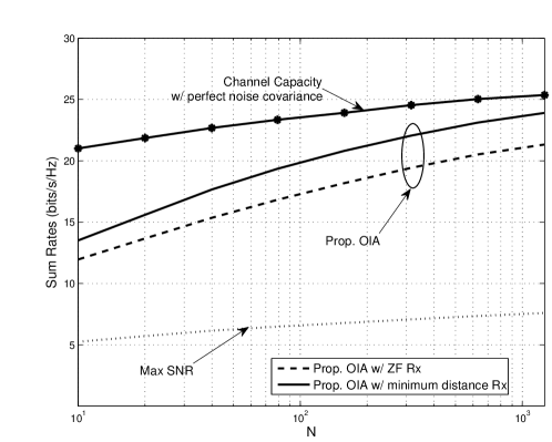
Figure 6: The achievable rate versus $N$ when $K=2$, $M=3$, $L=2$, $S=2$, SNR=20dB, and $n_{f}=6$. The random codebook is used.

Figure 6 shows a log-linear plot of the achievable rate versus $N$ when $K=2$, $M=3$, $L=2$, $S=2$, SNR=20dB, and $n_{f}=6$ when the random codebook is used. As shown in Theorem 3, it is seen that the GMI of the codebook-based OIA using the minimum Euclidean distance receiver asymptotically achieves the channel capacity as $N$ increases. On the other hand, the achievable rate of the codebook-based OIA using the ZF receiver exhibits a constant gap even in large $N$ regime, compared to that of the minimum Euclidean distance receiver. This observation is consistent with previous results on the single-user MIMO channel, showing that there exists a constant SNR gap between the channel capacity and the achievable rate based on the ZF receiver in the high SNR regime.

VII Conclusion

For the MIMO IMAC, we have proposed two different types of codebook-based OIA methods and analyzed the codebook size required to achieve the same user scaling condition and DoF as the SVD-based OIA case. We have shown that the required codebook size scaling is the same for both of the random and Grassmannian codebooks. In addition, we have shown that the simple minimum Euclidean distance receiver operating even with no CSI of inter-cell interfering links achieves the channel capacity as $N$ increases. Numerical examples have shown that it suffices for finite $n_{f}$ to almost obtain the achievable rate of the SVD-based OIA, e.g., the case where $n_{f}=8$ and $L=2$, and that the minimum Euclidean distance receiver enhances the achievable rate based on the ZF receiver especially in the low to mid SNR regimes.

Appendix A Proof of (IV-A)

By using $\nu_{f}\leq\textrm{SNR}^{-(1+\gamma)}$ in (18), $p_{c}$ defined in (21) can be lower-bounded by

$$p_{c} \geq\textrm{Pr}\left\{{\sigma^{[i,j]}_{L}}^{2}\geq(1+\delta){\sigma^{[i,j]}_{1}}^{2}\textrm{SNR}^{-(1+\gamma)},\forall i\in\mathcal{K},j\in\mathcal{N}\right\}$$

$$=\left(\textrm{Pr}\left\{\frac{{\sigma^{[i,j]}_{1}}^{2}}{{\sigma^{[i,j]}_{L}}^{2}}\leq(1+\delta)^{-1}\textrm{SNR}^{1+\gamma}\right\}\right)^{KN},$$ (56)

where (56) comes from the fact that $\mathbf{G}^{[i,j]}$ is independent for different $i$ or $j$, and thus their singular values are independent for different users. Note that $\frac{{\sigma^{[i,j]}_{1}}^{2}}{{\sigma^{[i,j]}_{L}}^{2}}$ is the condition number of ${\mathbf{G}^{[i,j]}}^{\textrm{H}}\mathbf{G}^{[i,j]}$. At this point, we introduce the following lemma on the CDF of the condition number.

Lemma 5

The CDF of $\frac{{\sigma^{[i,j]}_{1}}^{2}}{{\sigma^{[i,j]}_{L}}^{2}}$, denoted by $F_{c}(x)$, is lower-bounded by

$$F_{c}(x)\geq 1-\rho x^{-((K-1)S-L+1)},$$ (57)

where $\rho$ is a constant determined by $K$, $S$, and $L$.

Proof:

Since each channel coefficient is assumed to be chosen from a continuous distribution, $\mathbf{G}^{[i,j]}$ has full rank almost surely [33]. Moreover, assuming that $(K-1)S>L$, ${\mathbf{G}^{[i,j]}}^{\textrm{H}}\mathbf{G}^{[i,j]}$ is the full-rank central Wishart matrix, i.e., ${\mathbf{G}^{[i,j]}}^{\textrm{H}}\mathbf{G}^{[i,j]}\sim\mathcal{CW}_{L}\left((K-1)S,\mathbf{I}_{L}\right)$. Using the high-tail distribution of the complementary CDF in [34, Theorem 4], the CDF is bounded by (57), where $\rho=\left(\sum_{l=1}^{L}\kappa_{l}\mu_{l}\right)$. Here, $\kappa_{l}=\frac{(-1)^{l(l-1)/2}}{((K-1)S-L+1)!}$ and $\mu_{l}=\int_{0}^{\infty}\lambda_{1}^{((K-1)S-L+1)}g_{L-1,(K-1)S}(\lambda_{1})d\lambda_{1}$, where $\lambda_{1}\triangleq{\sigma^{[i,j]}_{1}}^{2}$ and $g_{L-1,(K-1)S}(\cdot)$ denotes the distribution of the largest eigenvalue of a reduced Wishart matrix $\tilde{\mathbf{G}}\sim\mathcal{CW}_{L-1}\left((K-1)S,\mathbf{I}_{L-1}\right)$. Thus, $\rho$ is determined only by $K$, $S$, and $L$. ∎

Now, from Lemma 5, (56) is further bounded by

$$p_{c} \!\geq\!\left(1\!-\!\rho(1+\delta)^{(K-1)S+L-1}\textrm{SNR}^{-(1+\gamma)((K-1)S-L+1)}\right)^{KN}$$

$$\geq 1\!-\!\rho KN(1+\delta)^{(K-1)S+L-1}\textrm{SNR}^{-(1+\gamma)((K-1)S-L+1)},$$ (58)

where (58) follows from $(1-x)^{y}>1-xy$ for any $0<x<1<y$. Therefore, if $N$ scales slower than $\textrm{SNR}^{(1+\gamma)((K-1)S-L+1)}$ for given $\gamma$, i.e., $N=O\left(\textrm{SNR}^{(1+\beta)((K-1)S-L+1)}\right)$ where $\beta<\gamma$, then $\lim_{\textrm{SNR}\rightarrow\infty}p_{c}\rightarrow 1$ for any given $\delta$, which proves the argument (IV-A).

Appendix B Proof of Lemma 4

Let us first consider the numerator of the logarithmic term in (41) as follows.

$$E\left[\operatorname{log}_{2}Q(\tilde{\mathbf{y}}_{i}|\mathbf{x}_{i})^{\theta}|\tilde{\mathbf{H}}_{i}\right] =-\frac{\theta}{\operatorname{log}2}E\left[(\tilde{\mathbf{y}}_{i}-\tilde{\mathbf{H}}_{i}\mathbf{x}_{i})^{\textrm{H}}\hat{\mathbf{R}}^{-1}(\tilde{\mathbf{y}}_{i}-\tilde{\mathbf{H}}_{i}\mathbf{x}_{i})\big{|}\tilde{\mathbf{H}}_{i}\right]$$

$$=-\frac{\theta}{\operatorname{log}2}E\left[\tilde{\mathbf{z}}_{i}^{\textrm{H}}\hat{\mathbf{R}}^{-1}\tilde{\mathbf{z}}_{i}\big{|}\tilde{\mathbf{H}}_{i}\right]$$

$$=-\frac{\theta}{\operatorname{log}2}\textrm{tr}(\hat{\mathbf{R}}^{-1/2}\mathbf{R}\hat{\mathbf{R}}^{-1/2}),$$ (59)

where (59) follows from $E[\mathbf{z}^{\textrm{H}}\mathbf{A}\mathbf{z}]=\textrm{tr}(\mathbf{A}^{1/2}\mathbf{R}\mathbf{A}^{1/2})$ for any random vector $\mathbf{z}$ with $E\{\mathbf{z}\mathbf{z}^{\textrm{H}}\}=\mathbf{R}$ and $E\{\mathbf{z}\}=\mathbf{0}$ and for any conjugate symmetric matrix $\mathbf{A}$.

Let us turn to the denominator of the logarithmic term in (41). Here, given that $\tilde{\mathbf{H}}_{i}$ and $\tilde{\mathbf{y}}_{i}$ are deterministic, the expectation is taken over $\mathbf{x}_{i}$. Since $\mathbf{x}_{i}$ is an $S$-dimensional complex Gaussian random vector, i.e., the probability density function of $\mathbf{x}_{i}$ is given by $1/\pi^{S}\operatorname{exp}\left(-\|\mathbf{x}_{i}\|^{2}\right)$, we have

$$E\left[Q(\tilde{\mathbf{y}}_{i}|\mathbf{x}_{i})^{\theta}\big{|}\tilde{\mathbf{y}}_{i},\tilde{\mathbf{H}}_{i}\right]$$

$$=\int\operatorname{exp}\left(-\theta(\tilde{\mathbf{y}}_{i}-\tilde{\mathbf{H}}_{i}\mathbf{x}_{i})^{\textrm{H}}\hat{\mathbf{R}}^{-1}(\tilde{\mathbf{y}}_{i}-\tilde{\mathbf{H}}_{i}\mathbf{x}_{i})\right)\frac{1}{\pi^{S}}\operatorname{exp}\left(-\|\mathbf{x}_{i}\|^{2}\right)d\mathbf{x}_{i}$$

$$=\frac{1}{\pi^{S}}\int\operatorname{exp}\bigl{(}-\theta(\tilde{\mathbf{y}}_{i}-\tilde{\mathbf{H}}_{i}\mathbf{x}_{i})^{\textrm{H}}\hat{\mathbf{R}}^{-1}(\tilde{\mathbf{y}}_{i}-\tilde{\mathbf{H}}_{i}\mathbf{x}_{i})-\|\mathbf{x}_{i}\|^{2}\bigr{)}d\mathbf{x}_{i}$$

$$=\frac{1}{\pi^{S}}\int\operatorname{exp}\left(-A\right)d\mathbf{x}_{i}.$$ (60)

Here, $A$ can be further expressed as

$$A \triangleq\theta(\tilde{\mathbf{y}}_{i}-\tilde{\mathbf{H}}_{i}\mathbf{x}_{i})^{\textrm{H}}\hat{\mathbf{R}}^{-1}(\tilde{\mathbf{y}}_{i}-\tilde{\mathbf{H}}_{i}\mathbf{x}_{i})+\|\mathbf{x}_{i}\|^{2}$$

$$=\mathbf{x}_{i}^{\textrm{H}}(\theta\tilde{\mathbf{H}}_{i}^{\textrm{H}}\hat{\mathbf{R}}^{-1}\tilde{\mathbf{H}}_{i}+\mathbf{I}_{S})\mathbf{x}_{i}-\theta\tilde{\mathbf{y}}_{i}^{\textrm{H}}\hat{\mathbf{R}}^{-1}\tilde{\mathbf{H}}_{i}\mathbf{x}_{i}-\theta\mathbf{x}_{i}^{\textrm{H}}\tilde{\mathbf{H}}_{i}^{\textrm{H}}\hat{\mathbf{R}}^{-1}\tilde{\mathbf{y}}_{i}+\theta\tilde{\mathbf{y}}_{i}^{\textrm{H}}\hat{\mathbf{R}}^{-1}\tilde{\mathbf{y}}_{i}.$$ (61)

Letting $\tilde{\boldsymbol{\Omega}}=\theta\tilde{\mathbf{H}}_{i}^{\textrm{H}}\hat{\mathbf{R}}^{-1}\tilde{\mathbf{H}}_{i}+\mathbf{I}_{S}$, it follows that

$$A =\left\|\tilde{\boldsymbol{\Omega}}^{1/2}\mathbf{x}_{i}-\mathbf{C}\tilde{\mathbf{y}}_{i}\right\|^{2}+\theta\tilde{\mathbf{y}}_{i}^{\textrm{H}}\hat{\mathbf{R}}^{-1}\tilde{\mathbf{y}}_{i}-\tilde{\mathbf{y}}_{i}^{\textrm{H}}\mathbf{C}^{\textrm{H}}\mathbf{C}\tilde{\mathbf{y}}_{i},$$ (62)

where $\mathbf{C}$ is given by $\mathbf{C}=\theta\tilde{\boldsymbol{\Omega}}^{-1/2}\tilde{\mathbf{H}}_{i}^{H}\hat{\mathbf{R}}^{-1}$, which comes from the equivalence of (61) and (62). Now let us further simplify the last two terms of (62) as

$$\theta\tilde{\mathbf{y}}_{i}^{\textrm{H}}\hat{\mathbf{R}}^{-1}\tilde{\mathbf{y}}_{i}-\tilde{\mathbf{y}}_{i}^{\textrm{H}}\mathbf{C}^{\textrm{H}}\mathbf{C}\tilde{\mathbf{y}}_{i} =\theta\tilde{\mathbf{y}}_{i}^{\textrm{H}}\left(\hat{\mathbf{R}}^{-1}-\theta\hat{\mathbf{R}}^{-1}\tilde{\mathbf{H}}_{i}\tilde{\boldsymbol{\Omega}}^{-1}\tilde{\mathbf{H}}_{i}^{\textrm{H}}\hat{\mathbf{R}}^{-1}\right)\tilde{\mathbf{y}}_{i}$$

$$=\theta\tilde{\mathbf{y}}_{i}^{\textrm{H}}\hat{\mathbf{R}}^{-1/2}\left(\mathbf{I}_{S}-\theta\hat{\mathbf{R}}^{-1/2}\tilde{\mathbf{H}}_{i}\tilde{\boldsymbol{\Omega}}^{-1}\tilde{\mathbf{H}}_{i}^{\textrm{H}}\hat{\mathbf{R}}^{-1/2}\right)\hat{\mathbf{R}}^{-1/2}\tilde{\mathbf{y}}_{i}.$$

Without loss of generality, it follows that $\hat{\mathbf{R}}^{-1/2}\tilde{\mathbf{H}}_{i}=\boldsymbol{\Phi}\boldsymbol{\Lambda}\mathbf{T}^{\textrm{H}}$, where $\boldsymbol{\Phi}\in\mathbb{C}^{S\times S}$ and $\mathbf{T}\in\mathbb{C}^{S\times S}$ are orthogonal matrices and $\boldsymbol{\Lambda}$ is an $(S\times S)$-dimensional diagonal matrix. Then, we get

$$\tilde{\boldsymbol{\Omega}}=\theta\tilde{\mathbf{H}}_{i}^{\textrm{H}}\hat{\mathbf{R}}^{-1}\tilde{\mathbf{H}}_{i}+\mathbf{I}_{S}=\mathbf{T}\left(\theta\boldsymbol{\Lambda}^{2}+\mathbf{I}_{S}\right)\mathbf{T}^{\textrm{H}}.$$ (63)

Inserting (63) to $\hat{\mathbf{R}}^{-1/2}\tilde{\mathbf{H}}_{i}\tilde{\boldsymbol{\Omega}}^{-1}\tilde{\mathbf{H}}_{i}^{\textrm{H}}\hat{\mathbf{R}}^{-1/2}$ gives us

$$\hat{\mathbf{R}}^{-1/2}\tilde{\mathbf{H}}_{i}\tilde{\boldsymbol{\Omega}}^{-1}\tilde{\mathbf{H}}_{i}^{\textrm{H}}\hat{\mathbf{R}}^{-1/2} =\boldsymbol{\Phi}\boldsymbol{\Lambda}^{2}\left(\theta\boldsymbol{\Lambda}^{2}+\mathbf{I}_{S}\right)^{-1}\boldsymbol{\Phi}^{\textrm{H}},$$

which yields

$$\theta\tilde{\mathbf{y}}_{i}^{\textrm{H}}\hat{\mathbf{R}}^{-1}\tilde{\mathbf{y}}_{i}-\tilde{\mathbf{y}}_{i}^{\textrm{H}}\mathbf{C}^{\textrm{H}}\mathbf{C}\tilde{\mathbf{y}}_{i} =\theta\tilde{\mathbf{y}}_{i}^{\textrm{H}}\hat{\mathbf{R}}^{-1/2}\boldsymbol{\Phi}\left(\mathbf{I}_{S}-\theta\boldsymbol{\Lambda}^{2}\left(\theta\boldsymbol{\Lambda}^{2}+\mathbf{I}_{S}\right)^{-1}\right)\boldsymbol{\Phi}^{\textrm{H}}\hat{\mathbf{R}}^{-1/2}\tilde{\mathbf{y}}_{i}$$

$$=\theta\tilde{\mathbf{y}}_{i}^{\textrm{H}}\hat{\mathbf{R}}^{-1/2}\boldsymbol{\Phi}\left(\theta\boldsymbol{\Lambda}^{2}+\mathbf{I}_{S}\right)^{-1}\boldsymbol{\Phi}^{\textrm{H}}\hat{\mathbf{R}}^{-1/2}\tilde{\mathbf{y}}_{i}$$ (64)

$$=\theta\tilde{\mathbf{y}}_{i}^{\textrm{H}}\hat{\mathbf{R}}^{-1/2}\left(\theta\hat{\mathbf{R}}^{-1/2}\tilde{\mathbf{H}}_{i}\tilde{\mathbf{H}}_{i}^{\textrm{H}}\hat{\mathbf{R}}^{-1/2}+\mathbf{I}_{S}\right)^{-1}\hat{\mathbf{R}}^{-1/2}\tilde{\mathbf{y}}_{i}$$

$$=\theta\tilde{\mathbf{y}}_{i}^{\textrm{H}}\left(\theta\tilde{\mathbf{H}}_{i}\tilde{\mathbf{H}}_{i}^{\textrm{H}}+\hat{\mathbf{R}}\right)^{-1}\tilde{\mathbf{y}}_{i}$$

$$=\theta\tilde{\mathbf{y}}_{i}^{\textrm{H}}\boldsymbol{\Omega}^{-1}\hat{\mathbf{R}}^{-1}\tilde{\mathbf{y}}_{i},$$ (65)

where (64) follows immediately from evaluating the diagonal terms, and (65) follows from $\boldsymbol{\Omega}\triangleq\theta\hat{\mathbf{R}}^{-1}\tilde{\mathbf{H}}_{i}\tilde{\mathbf{H}}_{i}^{\textrm{H}}+\mathbf{I}_{S}$. Inserting (65) and (62) to (60) gives us

$$E\left[Q(\tilde{\mathbf{y}}_{i}|\mathbf{x}_{i})^{\theta}|\tilde{\mathbf{y}}_{i},\tilde{\mathbf{H}}_{i}\right]$$

$$=\frac{1}{\pi^{S}}\int\operatorname{exp}\left(\!-\!\left\|\tilde{\boldsymbol{\Omega}}^{1/2}\mathbf{x}_{i}\!-\!\mathbf{C}\tilde{\mathbf{y}}_{i}\right\|^{2}\!-\!\theta\tilde{\mathbf{y}}_{i}^{\textrm{H}}\boldsymbol{\Omega}^{-1}\hat{\mathbf{R}}^{-1}\tilde{\mathbf{y}}_{i}\!\right)d\mathbf{x}_{i}$$

$$=\frac{1}{\pi^{S}}\operatorname{exp}\left(-\theta\tilde{\mathbf{y}}_{i}^{\textrm{H}}\boldsymbol{\Omega}^{-1}\hat{\mathbf{R}}^{-1}\tilde{\mathbf{y}}_{i}\right)\int\operatorname{exp}\left(-\left\|\tilde{\boldsymbol{\Omega}}^{1/2}\mathbf{x}_{i}-\mathbf{C}\tilde{\mathbf{y}}_{i}\right\|^{2}\right)d\mathbf{x}_{i}$$

$$=\frac{1}{\pi^{S}}\operatorname{exp}\left(-\theta\tilde{\mathbf{y}}_{i}^{\textrm{H}}\boldsymbol{\Omega}^{-1}\hat{\mathbf{R}}^{-1}\tilde{\mathbf{y}}_{i}\right)\pi^{S}\det\left(\tilde{\boldsymbol{\Omega}}^{-1}\right)$$ (66)

$$=\operatorname{exp}\left(-\theta\tilde{\mathbf{y}}_{i}^{\textrm{H}}\boldsymbol{\Omega}^{-1}\hat{\mathbf{R}}^{-1}\tilde{\mathbf{y}}_{i}\right)\det\left(\boldsymbol{\Omega}^{-1}\right),$$ (67)

where (66) follows from the fact that for $\mathbf{x},\mathbf{m}\in\mathbb{C}^{S\times 1}$ and conjugate symmetric $\mathbf{A},\mathbf{B}\in\mathbb{C}^{S\times S}$,

$$\int\operatorname{exp}\left(-(\mathbf{A}\mathbf{x}-\mathbf{m})^{\textrm{H}}\mathbf{B}^{-1}(\mathbf{A}\mathbf{x}-\mathbf{m})\right)d\mathbf{x}$$

$$=\int\operatorname{exp}\left(-(\mathbf{x}-\mathbf{A}^{-1}\mathbf{m})^{\textrm{H}}\mathbf{A}^{\textrm{H}}\mathbf{B}^{-1}\mathbf{A}(\mathbf{x}-\mathbf{A}^{-1}\mathbf{m})\right)d\mathbf{x}$$

$$=\pi^{S}\det\left(\mathbf{A}^{-1}\mathbf{B}(\mathbf{A}^{\textrm{H}})^{-1}\right),$$

and (67) follows from $\det(\tilde{\boldsymbol{\Omega}})=\det(\boldsymbol{\Omega})$. Inserting (59) and (67) to (41) gives us

$$I(\theta) =-\frac{\theta}{\operatorname{log}2}\textrm{tr}(\hat{\mathbf{R}}^{-1/2}\mathbf{R}\hat{\mathbf{R}}^{-1/2})-E\left[\operatorname{log}_{2}\left(\operatorname{exp}\left(-\theta\tilde{\mathbf{y}}_{i}^{\textrm{H}}\boldsymbol{\Omega}^{-1}\hat{\mathbf{R}}^{-1}\tilde{\mathbf{y}}_{i}\right)\det\left(\boldsymbol{\Omega}^{-1}\right)\right)\big{|}\tilde{\mathbf{H}}_{i}\right]$$

$$=-\frac{\theta}{\operatorname{log}2}\textrm{tr}(\hat{\mathbf{R}}^{-1/2}\mathbf{R}\hat{\mathbf{R}}^{-1/2})+\frac{\theta}{\operatorname{log}2}E\left[\tilde{\mathbf{y}}_{i}^{\textrm{H}}\boldsymbol{\Omega}^{-1}\hat{\mathbf{R}}^{-1}\tilde{\mathbf{y}}_{i}\big{|}\tilde{\mathbf{H}}_{i}\right]+\operatorname{log}_{2}\det(\boldsymbol{\Omega}).$$

From

$$E\left[\tilde{\mathbf{y}}_{i}^{\textrm{H}}\boldsymbol{\Omega}^{-1}\hat{\mathbf{R}}^{-1}\tilde{\mathbf{y}}_{i}\big{|}\tilde{\mathbf{H}}_{i}\right] =E\left[\left(\mathbf{x}_{i}^{\textrm{H}}\tilde{\mathbf{H}}_{i}^{\textrm{H}}+\mathbf{z}_{i}^{\textrm{H}}\right)\boldsymbol{\boldsymbol{\Omega}}^{-1}\hat{\mathbf{R}}^{-1}\left(\tilde{\mathbf{H}}_{i}\mathbf{x}_{i}+\mathbf{z}_{i}\right)\right]$$

$$=\textrm{tr}\left(\boldsymbol{\Omega}^{-1}\hat{\mathbf{R}}^{-1}\tilde{\mathbf{H}}_{i}\tilde{\mathbf{H}}_{i}^{\textrm{H}}\right)+\textrm{tr}\left(\boldsymbol{\Omega}^{-1}\hat{\mathbf{R}}^{-1}\mathbf{R}\right),$$

we finally have

$$I(\theta) =-\frac{\theta}{\operatorname{log}2}\textrm{tr}(\hat{\mathbf{R}}^{-1/2}\mathbf{R}\hat{\mathbf{R}}^{-1/2})+\frac{\theta}{\operatorname{log}2}\bigl{[}\textrm{tr}\left(\boldsymbol{\Omega}^{-1}\hat{\mathbf{R}}^{-1}\tilde{\mathbf{H}}_{i}\tilde{\mathbf{H}}_{i}^{\textrm{H}}\right)+\textrm{tr}\left(\boldsymbol{\Omega}^{-1}\hat{\mathbf{R}}^{-1}\mathbf{R}\right)\bigr{]}+\operatorname{log}_{2}\det(\boldsymbol{\Omega}),$$

which completes the proof of the lemma.

References

• [1] V. R. Cadambe and S. A. Jafar, “Interference alignment and degrees of freedom of the K-user interference channel,” IEEE Trans. Inf. Theory, vol. 54, no. 8, pp. 3425–3441, Aug. 2008.
• [2] M. A. Maddah-Ali, A. S. Motahari, and A. K. Khandani, “Communication over MIMO X channels: Interference alignment, decomposition, and performance analysis,” IEEE Trans. Inf. Theory, vol. 54, no. 8, pp. 3457–3470, Aug. 2008.
• [3] B. C. Jung and W.-Y. Shin, “Opportunistic interference alignment for interference-limited cellular TDD uplink,” IEEE Commun. Lett., vol. 15, no. 2, pp. 148–150, Feb. 2011.
• [4] B. C. Jung, D. Park, and W.-Y. Shin, “Opportunistic interference mitigation achieves optimal degrees-of-freedom in wireless multi-cell uplink networks,” IEEE Trans. Commun., vol. 60, no. 7, pp. 1935–1944, Jul. 2012.
• [5] C. Suh and D. Tse, “Interference alignment for cellular networks,” in Proc. 46th Annual Allerton Conf. Communication, Control, and Computing, Urbana-Champaign, IL, Sept. 2008, pp. 1037 – 1044.
• [6] K. Gomadam, V. R. Cadambe, and S. A. Jafar, “A distributed numerical approach to interference alignment and applications to wireless interference networks,” IEEE Trans. Inf. Theory, vol. 57, no. 6, pp. 3309–3322, June 2011.
• [7] H. J. Yang, W.-Y. Shin, B. C. Jung, and A. Paulraj, “Opportunistic interference alignment of MIMO interfering multiple-access channels,” IEEE Trans. Wireless Commun., vol. 12, no. 5, pp. 2180–2192, May 2013.
• [8] ——, “Opportunistic interference alignment of MIMO IMAC : Effect of user scaling over degrees-of-freedom,” in Proc. IEEE Int’l Symp. Inf. Theory (ISIT), Cambridge, MA, July 2012, pp. 2646–2650.
• [9] J. Thukral and H. Bölcskei, “Interference alignment with limited feedback,” in Proc. IEEE Int’l Symp. Inf. Theory (ISIT), Seoul, Korea, July 2009, pp. 1759–1763.
• [10] R. T. Krishnamachari and M. K. Varanasi, “Interference alignment under limited feedback for MIMO interference channels,” in Proc. IEEE Int’l Symp. Inf. Theory (ISIT), Austin, TX, June 2010, pp. 619–623.
• [11] B. Mondal and R. W. Heath, Jr., “Performance analysis of quantized beamforming MIMO systems,” IEEE Trans. Signal Process., vol. 54, no. 12, pp. 4753–4766, Dec. 2006.
• [12] T. Yoo, N. Jindal, and A. Goldsmith, “Multi-antenna downlink channels with limited feedback and user selection,” IEEE J. Select. Areas Commun., vol. 25, no. 7, pp. 1478–1491, Sept. 2007.
• [13] N. Jindal, “MIMO broadcast channels with finite-rate feedback,” IEEE Trans. Inf. Theory, vol. 52, no. 11, pp. 5045–5060, Nov. 2006.
• [14] TS 36.213, Evolved Universal Terrestrial Radio Access (E-UTRA); Physical layer procedures, 3GPP Std., v.11.2.0.
• [15] L. Choi and R. D. Murch, “A transmit preprocessing technique for multiuser MIMO systems using a decomposition approach,” IEEE Trans. Wireless Commun., vol. 3, no. 1, pp. 20–24, Jan. 2004.
• [16] Z. Pan, K.-K. Wong, and T.-S. Ng, “Generalized multiuser orthogonal space-division multiplexing,” IEEE Trans. Wireless Commun., vol. 3, no. 6, pp. 1969–1973, Nov. 2004.
• [17] TS 36.212, Evolved Universal Terrestrial Radio Access (E-UTRA); Multiplexing and channel coding, 3GPP Std., v.11.2.0.
• [18] C.-B. Chae, D. Mazzarese, T. Inoue, and R. W. Heath, Jr., “Coordinated beamforming for the multiuser MIMO broadcast channel with limited feedforward,” IEEE Trans. Signal Process., vol. 56, no. 12, pp. 6044–6056, Dec. 2008.
• [19] “Apparatus and method for beamforming with limited feedforward channel in multiple input multiple output wireless communication system,” US Patent 7786934, Aug. 2010.
• [20] J. Jose, A. Ashikhmin, P. Whiting, and S. Vishwanath, “Channel estimation and linear precoding in multiuser multiple-antenna TDD systems,” IEEE Trans. Veh. Technol., vol. 60, no. 5, pp. 2102–2116, June 2011.
• [21] D. Samardzija, L. Xiao, and N. Mandayam, “Impact of pilot assisted channel state estimation on multiple antenna multiuser TDD systems with spatial filtering,” in Proc. 40th Annual Conf. Information Sciences and Systems, Lucent Technol. Bell Labs, Holmdel, NJ, Mar. 2006, pp. 381–385.
• [22] J. Jose, A. Ashikhmin, T. L. Marzetta, and S. Vishwanath, “Pilot contamination and precoding in multi-cell TDD systems,” IEEE Trans. Wireless Commun., vol. 10, no. 8, pp. 2640–2651, Aug. 2011.
• [23] L. Soriano-Equigua, J. Sánchez-García, J. Flores-Troncoso, and R. W. Heath, Jr., “Noniterative coordinated beamforming for multiuser MIMO systems with limited feedforward,” IEEE Signal Process. Lett., vol. 18, no. 12, pp. 701–704, Dec. 2011.
• [24] D. J. Love and R. W. Heath, Jr., “Grassmannian beamforming for multiple-input multple-output wireless systems,” IEEE Trans. Inf. Theory, vol. 49, no. 10, pp. 2735–2747, Oct. 2003.
• [25] W. Dai, Y. E. Liu, and B. Rider, “Quantization bounds on Grassmann manifolds and applications to MIMO communications,” IEEE Trans. Inf. Theory, vol. 54, no. 3, pp. 1108–1123, Mar. 2008.
• [26] A. Barg and D. Y. Nogin, “Bounds on packings of spheresin the Grassmann manifold,” IEEE Trans. Inf. Theory, vol. 48, no. 9, pp. 2450–2454, Sept. 2002.
• [27] S. Jin, M. R. McKay, X. Gao, and I. B. Collings, “MIMO multichannel beamforming: SER and outage using new eigenvalue distributions of complex noncentral Wishart matrices,” IEEE Trans. Commun., vol. 56, no. 3, pp. 424–434, Mar. 2008.
• [28] C. K. Au-Yeung and D. J. Love, “Optimization and tradeoff analysis of two-way limited feedback beamforming systems,” IEEE Trans. Wireless Commun., vol. 8, no. 5, pp. 2570–2579, May 2009.
• [29] B. Khoshnevis, “Multiple-antenna communications with limited channel state information,” Ph.D. dissertation, University of Toronto, 2011.
• [30] R. S. Blum, “MIMO capacity with interference,” IEEE J. Selec. Area. Commun., vol. 21, no. 5, pp. 793–801, June 2003.
• [31] A. Ganti, A. Lapidoth, and I. E. Telatar, “Mismatched decoding revisited: General alphabets, channels with memory, and the wide-band limit,” IEEE Trans. Inf. Theory, vol. 46, no. 7, pp. 2315–2328, Nov. 2000.
• [32] N. Merhav, G. Kaplan, A. Lapidoth, and S. Shamai (Shitz), “On information rates for mismatched decoders,” IEEE Trans. Inf. Theory, vol. 40, no. 6, pp. 1953–1967, Nov. 1994.
• [33] A. Edelman, “Eigenvalues and condition numbers of random matrices,” Ph.D. dissertation, Messachusetts Institute of Technology, 1989.
• [34] M. Matthaiou, M. R. McKay, P. J. Smith, and J. A. Nossek, “On the condition number distribution of complex Wishart matrices,” IEEE Trans. Commun., vol. 58, no. 6, pp. 1705–1717, June 2010.