Canonical duality for solving general nonconvex constrained problems

Abstract

This paper presents a canonical duality theory for solving a general nonconvex constrained optimization problem within a unified framework to cover Lagrange multiplier method and KKT theory. It is proved that if both target function and constraints possess certain patterns necessary for modeling real systems, a perfect dual problem (without duality gap) can be obtained in a unified form with global optimality conditions provided. While the popular augmented Lagrangian method may produce more difficult nonconvex problems due to the nonlinearity of constraints.

1 Introduction

We are interested in solving the following nonconvex constrained minimization problem:

$$\begin{array}[]{lll}\min&f(x)\\ s.t.&g_{i}(x)\leq 0&i=1,\dots,m\\ &h_{j}(x)=0&j=1,\dots,p,\end{array}$$ (1)

where $f$, $g_{i}$ and $h_{j}$ are smooth, real-valued functions on a subset of ⁿ for all $i=1,\dots,m$ and $j=1,\dots,p$. For notational convenience, we use vector form for constraints $g(x)$ and $h(x)$ (without the subscript):

$$\begin{array}[]{l}g(x)=\left(g_{1}(x),\dots,g_{m}(x)\right),\\ h(x)=\left(h_{1}(x),\dots,h_{p}(x)\right).\end{array}$$

Therefore, the feasible space can be defined as

$${\cal X}_{a}:=\{x\in{}^{n}|g(x)\leq 0,h(x)=0\}.$$

Lagrange multiplier method was originally proposed by J-L. Lagrange from analytical mechanics in 1811 lag . During the past two hundred years, this method and the associated Lagrangian duality theory have been well-developed with extensively applications to many fields of physics, mathematics and engineering sciences. Strictly speaking, the Lagrange multiplier method can be used only for equilibrium constraints. For inequality constraints, the additional KKT conditions should be considered. In order to solve inequality constrained problems, penalty methods and augmented Lagrangian methods have been studied extensively during the past fifty years (see powell ; bgm2005 ; aug2000 ). However, these well-developed methods can be used mainly for solving linear inequality constrained problems. For nonlinear constraints, say even the most simple quadratic constraint $\|x\|^{2}\leq r$ which is essential for virtually any real-world system chen-gao-OMS , the (external) penalty/augmented Lagrangian methods produce a nonconvex term $\frac{1}{2}\alpha(\|x\|^{2}-r)^{2}_{+}$ in the problem.

Canonical duality theory is potentially powerful methodological method, which was developed originally from nonconvex analysis/mechanics GaoBook 2000 ; gao-jogo00 . This theory has been used successfully for solving a large class of challenging problems in nonconvex/nonsmooth/discrete systems gao-cace09 ; wang-etal ; zgy , recently in network communications g-r-p ; ruan-gao-ep and radial basis neural networks LaG 13 . It was shown in gao-sherali-amma that both the Lagrange multiplier method and KKT conditions can be unified within a framework of the canonical duality theory. This unified framework leads to an elegant and simple way to handle nonlinear constrained optimization problems. The associated triality theory provides global optimal conditions which can be used to develop efficient algorithms for solving general nonconvex constrained problems (see gao-ruan-sherali-jogo ; gao-yang ).

The canonical duality theory for solving nonconvex constrained quadratic minimization problem has been discussed in gao-ruan-sherali-jogo . The main goal of this paper is to demonstrate how to use the canonical duality theory for solving the general non-convex constrained problem (1).

2 Unity for Convex Problems

For a given convex feasible set $\cal E$, its indicator function $\Psi(\epsilon)$ is defined by

$$\Psi(\epsilon)=\begin{cases}0\qquad\mbox{if }\epsilon\in{\cal E}\\ +\infty\quad\mbox{otherwise}.\end{cases}$$ (2)

The Legendre conjugate of $\Psi(\epsilon)$ is defined by using the Fenchel transformation

$$\Psi^{*}(\epsilon^{*})=\sup_{\epsilon\in\cal E}\{\epsilon^{T}\epsilon^{*}-\Psi(\epsilon)\}\quad\forall\epsilon^{*}\in{\cal E^{*}},$$ (3)

where ${\cal E^{*}}$ is a dual space of $\cal E$. Clearly, $\Psi^{*}(\epsilon^{*})$ is convex and lower semi-continuous. By the theory of convex analysis, the following canonical duality relations hold on ${\cal E}\times{\cal E^{*}}$:

$$\epsilon^{*}\in\partial\Psi(\epsilon)\quad\Leftrightarrow\quad\epsilon\in\partial\Psi^{*}(\epsilon^{*})\quad\Leftrightarrow\quad\Psi(\epsilon)+\Psi^{*}(\epsilon^{*})=\epsilon^{T}\epsilon^{*}.$$ (4)

A real-valued function is called the canonical function if the canonical duality relations (4) hold. Based on the standard canonical dual transformation, we choose the geometrical operator $\xi_{0}=\Lambda_{0}(x)=\{g(x),h(x)\}:{}^{n}\rightarrow{}^{2}$ and let

$$V_{0}(\xi_{0})=\Psi_{1}(g)+\Psi_{2}(h),$$

where

$$\Psi_{1}(g)=\begin{cases}0\qquad\mbox{if }g\leq 0\\ +\infty\quad\mbox{otherwise},\end{cases}\;\;\;\;\Psi_{2}(h)=\begin{cases}0\qquad\mbox{if }h=0\\ +\infty\quad\mbox{otherwise},\end{cases}$$ (5)

the constrained problem (1) can be written in the following canonical form

$$\min\left\{P(x)=f(x)+V_{0}(\Lambda_{0}(x))|\;\;\forall x\in\mathbb{R}\right\}.$$ (6)

By the Fenchel transformation, the conjugate of $V_{0}(\xi_{0})$ can be easily obtained as $V_{0}^{*}(\xi^{*}_{0})=\Psi^{*}_{1}(\lambda)+\Psi_{2}^{*}(\mu)$, where $\xi_{0}^{*}=(\lambda,\mu)$ and

$$\Psi_{1}^{*}(\lambda)=\sup_{g\in{}^{m}}\{g^{T}\lambda-\Psi_{1}(g)\}=\left\{\begin{array}[]{ll}0&\mbox{if }\lambda\geq 0\\ +\infty&\mbox{otherwise},\end{array}\right.$$

$$\Psi_{2}^{*}(\mu)=\sup_{h\in{}^{p}}\{h^{T}\mu-\Psi_{2}(h)\}=0\quad\forall\quad\mu\in{}^{p}.$$

By using the Fenchel-Young equality $V_{0}(\xi_{0})=\xi_{0}^{T}\xi_{0}^{*}-V_{0}^{*}(\xi_{0}^{*})$ to replace $V_{0}(\Lambda_{0}(x))$ in (6), the so called total complementarity function in the canonical duality theory can be obtained in the following form

$$\Xi_{0}(x,\lambda,\mu)=f(x)+[\lambda^{T}g(x)-\Psi_{1}^{*}(\lambda)]+[\mu^{T}h(x)-\Psi_{2}^{*}(\mu)].$$ (7)

For the indicator $\Psi_{1}(g)$, the canonical duality relations in (4) lead to

$$\begin{array}[]{llll}\lambda_{i}\in\partial\Psi_{1}(g_{i})&\Longrightarrow&\lambda\geq 0&i=1,\dots,m\\ g(x)\in\partial\Psi^{*}_{1}(\lambda)&\Longrightarrow&g_{i}\leq 0&i=1,\dots,m\\ \lambda^{T}g(x)=\Psi_{1}(g(x))+\Psi^{*}_{1}(\lambda)&\Longrightarrow&\lambda^{T}g=0,\end{array}$$ (8)

which are the KKT conditions for the inequality constrains $g(x)\leq 0$. While for $\Psi_{2}(h)$, the same relations in (4) lead to

$$\begin{array}[]{llll}\mu\in\partial\Psi_{2}(h_{j})&\Longrightarrow&\mu\in{}^{p}\\ h_{j}(x)\in\partial\Psi^{*}_{2}(\lambda)&\Longrightarrow&h_{j}=0&j=1,\dots,p\\ \mu^{T}h(x)=\Psi_{2}(g(x))+\Psi^{*}_{2}(\mu)&\Longrightarrow&\mu^{T}h=0.\end{array}$$ (9)

From the second and third equation in the (9), it is clear that in order to enforce the constrain $h(x)=0$, the dual variables $\mu_{i}$ must be not zero for $i=1,\dots,p$. This is a special complementarity condition for equality constrains, generally not mentioned in many textbooks. However, the implicit constraint $\mu\neq 0$ is important in nonconvex optimization. Let $\mbox{\boldmath$\sigma$}_{0}=(\lambda,\mu)$. The dual feasible spaces should be defined as

$${\cal S}_{0}=\{\mbox{\boldmath$\sigma$}_{0}=(\lambda,\mu)\in{}^{m\times p}|\;\;\lambda_{i}\geq 0\;\;\forall i=1,\dots,m,\;\;\mu_{j}\neq 0\;\;\forall j=1,\dots,p\}.$$

Thus, on the feasible space ${}^{n}\times{\cal S}_{0}$, the total complementary function (7) can be simplified as

$$\Xi_{0}(x,\mbox{\boldmath$\sigma$}_{0})=f(x)+\lambda^{T}g(x)+\mu^{T}h(x)={\cal L}(x,\lambda,\mu),$$ (10)

which is the classical Lagrangian form, and we have

$$P(x)=\sup\left\{\Xi_{0}(x,\mbox{\boldmath$\sigma$}_{0})|\;\forall\mbox{\boldmath$\sigma$}_{0}\in{\cal S}_{0}\right\}.$$

This shows that the canonical duality theory is an extension of the Lagrangian theory (actually, the total complementary function was called the extended Lagrangian in GaoBook 2000 ). With the canonical duality theory it is possible to formulate the optimality conditions for both inequality and equality constraints in an unified framework.

If $f$, $g$ are convex and $h$ is linear, the Lagrangian (10) is a saddle function, i.e. ${\cal L}(x,\lambda,\mu)$ is convex in the primal variable $x$ and concave(linear) in the dual variables $\lambda$ and $\mu$. In this case, the Lagrangian dual can be defined by

$$P^{*}(\lambda,\mu)=\inf_{x\in{\cal X}_{a}}{\cal L}(x,\lambda,\mu)$$

on a subspace ${\cal S}_{a}\subset{\cal S}_{0}$ and the saddle Lagrangian duality leads to the following strong duality relation

$$\inf_{x\in{\cal X}_{a}}{\cal L}(x,\lambda,\mu)=\sup_{(\lambda,\mu)\in{\cal S}_{a}}P^{*}(\lambda,\mu).$$

It is well-known that this Lagrangian duality holds only for convex problems. For general nonconvex constrained problems, only the weak duality relation is available, i.e. there is a duality gap between the primal problem and its Lagrangian dual. With the canonical duality theory, it is possible to close the duality gap to obtain global optimal solutions.

3 Sequential Transformation for Nonconvex Problems

In order to solve nonconvex constrained problems in a unified way, the nonconvex functions should be assumed to have certain patterns in order to model real-world problems. In this paper, we need the following assumption.

Assumption 1

The nonconvex functions $f$, $g_{i}$ and $h_{j}$ for $i=1,\dots,m$ and $j=1,\dots,p$ can be expressed in the following way:

$$\begin{array}[]{l}f(x)=V_{f}(\Lambda_{f}(x))+\frac{1}{2}x^{T}Ax-c^{T}x\\ g_{i}(x)=V_{g_{i}}(\Lambda_{g_{i}}(x))\quad i=1,\dots,m\\ h_{j}(x)=V_{h_{j}}(\Lambda_{h_{j}}(x))\quad j=1,\dots,p\end{array}$$

where $\xi_{f}=\Lambda_{f}(x)$, $\xi_{g_{i}}=\Lambda_{g_{i}}(x)$ and $\xi_{h_{j}}=\Lambda_{h_{j}}(x)$ are quadratic geometrical operators such that $V_{f}(\xi_{f})$, $V_{g_{i}}(\xi_{g_{i}})$, $V_{h_{j}}(\xi_{h_{j}})$ are differentiable canonical functions for every $i=1,\dots,m$ and $j=1,\dots,p$.

Based on this assumption, we can define the following second-level geometrical operators

$$\xi_{g}=\Lambda_{g}(x)=\left(\Lambda_{g_{i}},\dots,\Lambda_{g_{m}}\right),\;\;\quad\xi_{h}=\Lambda_{g}(x)=\left(\Lambda_{h_{j}},\dots,\Lambda_{h_{p}}\right).$$

Let $\xi_{1}=(\xi_{f},\xi_{g},\xi_{h})=\Lambda_{1}(x)$, $V_{g}(\xi_{g})=\{V_{g_{i}}(\xi_{g_{i}})\}$, and $V_{h}(\xi_{h})=\{V_{h_{i}}(\xi_{h_{i}})\}$. By Assumption 1, the following duality relations are invertible on their domains, respectively,

$$\xi^{*}_{f}=\nabla V_{f}(\xi_{f}),\;\;\xi^{*}_{g}=\nabla V_{g}(\xi_{g}),\;\;\xi^{*}_{h}=\nabla V_{h}(\xi_{h}).$$ (11)

Also, the Legendre conjugates $V^{*}_{f}(\xi_{f}^{*}),\;\;V^{*}_{g}(\xi^{*}_{g})$ and $V^{*}_{h}(\xi_{h}^{*})$ can be defined uniquely.

Denote $\mbox{\boldmath$\sigma$}_{1}=(\sigma_{f},\sigma_{g},\sigma_{h})=(\xi^{*}_{f},\xi^{*}_{g},\xi^{*}_{h})$ and let ${\cal S}_{1}$ be a domain such that on which, the inverse duality relations (11) hold. By using the Fenchel-Young equalities, the first-level total complementary function $\Xi_{0}$ (10) can be written in the following second-level form:

$$\Xi_{1}(x,\mbox{\boldmath$\sigma$}_{0},\mbox{\boldmath$\sigma$}_{1}) = \Lambda_{f}(x)\sigma_{f}-V^{*}_{f}(\sigma_{f})+\lambda^{T}(\Lambda_{g}(x)\circ\sigma_{g}-V^{*}_{g}(\sigma_{g}))$$ (12)

$$+\mu^{T}(\Lambda_{h}(x)\circ\sigma_{h}-V^{*}_{h}(\sigma_{h}))-U(x),$$

where $U(x)=c^{T}x-\frac{1}{2}x^{T}Ax$, and the symbol $\circ$ indicates the Hadamard product between the primal and dual variables, i.e.,

$$\xi_{g}\circ\sigma_{g}=\left(\xi_{g_{1}}\sigma_{g_{1}},\dots,\xi_{g_{m}}\sigma_{g_{m}}\right).$$

Based on (12), the canonical dual function can be obtained by

$$P^{d}(\mbox{\boldmath$\sigma$}_{0},\mbox{\boldmath$\sigma$}_{1})=U^{\Lambda}(\lambda,\mu,\sigma)-\left(V_{f}^{*}(\sigma_{f})+\lambda^{T}V_{g}^{*}(\sigma_{g})+\mu^{T}V_{h}^{*}(\sigma_{h})\right),$$ (13)

where $U^{\Lambda}(\mbox{\boldmath$\sigma$}_{0},\mbox{\boldmath$\sigma$}_{1})$ is the $\Lambda$-conjugate of $U(x)$ defined by (see GaoBook 2000 )

$$U^{\Lambda}(\mbox{\boldmath$\sigma$}_{0},\mbox{\boldmath$\sigma$}_{1})=\mbox{sta}\{\Lambda_{f}(x)\sigma_{f}+\lambda^{T}\left(\Lambda_{g}(x)\circ\sigma_{g}\right)+\mu^{T}\left(\Lambda_{h}(x)\circ\sigma_{h}\right)-U(x):x\in{}^{n}\}$$ (14)

Let ${\cal S}_{a}\subset{\cal S}_{0}\times{\cal S}_{1}$ be the canonical dual feasible space such that on which, $U^{\Lambda}(\mbox{\boldmath$\sigma$}_{0},\mbox{\boldmath$\sigma$}_{1})$ is well-defined. The canonical dual problem can be proposed as

$$({\cal P}^{d}):\quad\mbox{sta}\{P^{d}(\mbox{\boldmath$\sigma$}_{0},\mbox{\boldmath$\sigma$}_{1}):\;\;(\mbox{\boldmath$\sigma$}_{0},\mbox{\boldmath$\sigma$}_{1})\in{\cal S}_{a}\}.$$

$$\begin{array}[]{rlclc}&x&&x^{*}&\\[5.69046pt] \Lambda_{1}(x)&\left\downarrow\rule{0.0pt}{28.45274pt}\right.\phantom{(\varphi^{n})^{*}}&&\left\uparrow\rule{0.0pt}{28.45274pt}\right.\nabla\Lambda^{*}_{1}\\[5.69046pt] (\xi_{f},\xi_{g},\xi_{h})=&\xi_{1}\xleftrightarrow{\phantom{xxx}{\xi^{*}_{1}=\nabla V_{1}(\xi_{1})}\phantom{xxx}}&&\xi^{*}_{1}=\mbox{\boldmath$\sigma$}_{1}=(\sigma_{f},\sigma_{g},\sigma_{h})&\\[5.69046pt] \Lambda_{0}&\left\downarrow\rule{0.0pt}{28.45274pt}\right.\phantom{(\varphi^{n})^{*}}&&\left\uparrow\rule{0.0pt}{28.45274pt}\right.\xi_{1}^{*}=\mbox{\boldmath$\sigma$}_{1}(\mbox{\boldmath$\sigma$}_{0})\\[5.69046pt] (g,h)=&\xi_{0}\xleftrightarrow{\phantom{x}{\;\;\;\;\;\xi^{*}_{0}\;\;\in\;\;\partial V_{0}(\xi_{0})\;\;\;\;}\phantom{x}}&&\ \xi^{*}_{0}=\mbox{\boldmath$\sigma$}_{0}=(\lambda,\mu)&\\[5.69046pt] \end{array}$$

Figure 1: The scheme of the sequential canonical dual transformation.

Theorem 3.1

(Complementarity Dual Principle) Suppose that the point $(\bar{x},\bar{\mbox{\boldmath$\sigma$}}_{0},\bar{\mbox{\boldmath$\sigma$}}_{1})$ is a critical point for the total complementarity function (12), then $\bar{x}$ is a KKT point of the primal problem (1), $(\bar{\mbox{\boldmath$\sigma$}}_{0},\bar{\mbox{\boldmath$\sigma$}}_{1})$ is a KKT point of the dual problem (13) and

$$P(\bar{x})=\Xi_{1}(\bar{x},\bar{\mbox{\boldmath$\sigma$}}_{0},\bar{\mbox{\boldmath$\sigma$}}_{1})=P^{d}(\bar{\mbox{\boldmath$\sigma$}}_{0},\bar{\mbox{\boldmath$\sigma$}}_{1})$$

Proof

. If $(\bar{x},\bar{\mbox{\boldmath$\sigma$}}_{0},\bar{\mbox{\boldmath$\sigma$}}_{1})$ is a critical point for the total complementarity function (12) then it must satisfy the following first order conditions:

$$\nabla_{x}\Xi_{1}(\bar{x},\bar{\mbox{\boldmath$\sigma$}}_{0},\bar{\mbox{\boldmath$\sigma$}}_{1})= \nabla\Lambda_{f}(\bar{x})\bar{\sigma}_{f}+\bar{\lambda}^{T}(\nabla\Lambda_{g}(\bar{x})\circ\bar{\sigma}_{g})$$ (15)

$$+\bar{\mu}^{T}(\nabla\Lambda_{h}(\bar{x})\circ\bar{\sigma}_{h})+Ax-c=0,$$

$$\nabla_{\sigma_{f}}\Xi_{1}(\bar{x},\bar{\mbox{\boldmath$\sigma$}}_{0},\bar{\mbox{\boldmath$\sigma$}}_{1})= \Lambda_{f}(\bar{x})-\nabla V^{*}_{f}(\bar{\sigma}_{f})=0,$$

$$\nabla_{\sigma_{g}}\Xi_{1}(\bar{x},\bar{\mbox{\boldmath$\sigma$}}_{0},\bar{\mbox{\boldmath$\sigma$}}_{1})= \Lambda_{g}(\bar{x})-\nabla V^{*}_{g}(\bar{\sigma}_{h})=0,$$

$$\nabla_{\sigma_{h}}\Xi_{1}(\bar{x},\bar{\mbox{\boldmath$\sigma$}}_{0},\bar{\mbox{\boldmath$\sigma$}}_{1})= \Lambda_{h}(\bar{x})-\nabla V^{*}_{h}(\bar{\sigma}_{h})=0.$$

The last three conditions in the (15) are equivalent to

$$\bar{\sigma}_{f}=\nabla V_{f}\left(\Lambda_{f}(\bar{x})\right),\quad\bar{\sigma}_{g}=\nabla V_{g}\left(\Lambda_{g}(\bar{x})\right),\quad\bar{\sigma}_{h}=\nabla V_{h}\left(\Lambda_{f}(\bar{x})\right).$$

By substituting these conditions in the first equation of the (15) and using the chain rule of derivation on $f$, $g_{i}$ and $h_{j}$ for every $i=1,\dots,m$ and $j=1,\dots,p$, we obtain

$$\nabla f(\bar{x})+\bar{\lambda}^{T}\nabla g(\bar{x})+\bar{\mu}^{T}\nabla h(\bar{x})=\nabla{\cal L}(\bar{x},\bar{\lambda},\bar{\mu})=0.$$

This condition plus the conditions coming from the (8) prove that $\bar{x}$ is a KKT point for the (1). Furthermore, from these complementarity conditions we obtain that $f(\bar{x})=\Xi_{1}(\bar{x},\bar{\mbox{\boldmath$\sigma$}}_{0},\bar{\mbox{\boldmath$\sigma$}}_{1})$.

The first equation of the (15) leads to the satisfaction of the stationarity condition (14) that is:

$$U^{\Lambda}(\mbox{\boldmath$\sigma$}_{0},\mbox{\boldmath$\sigma$}_{1})=\Lambda_{f}(x)\sigma_{f}+\lambda^{T}\left(\Lambda_{g}(x)\circ\sigma_{g}\right)+\mu^{T}\left(\Lambda_{h}(x)\circ\sigma_{h}\right)-U(x).$$

This together with the property that the first order conditions of the dual are equivalent to the last three conditions of the (15) proves that $(\bar{\mbox{\boldmath$\sigma$}}_{0},\bar{\mbox{\boldmath$\sigma$}}_{1})=(\bar{\lambda},\bar{\mu},\bar{\sigma})$ is a KKT point of the dual and $\Xi_{1}(\bar{x},\bar{\mbox{\boldmath$\sigma$}}_{0},\bar{\mbox{\boldmath$\sigma$}}_{1})=P^{d}(\bar{\mbox{\boldmath$\sigma$}}_{0},\bar{\mbox{\boldmath$\sigma$}}_{1})$. ∎

This theorem shows that with the canonical duality theory and the sequential canonical dual transformation it is possible to close the duality gap between the nonconvex primal problem and its canonical dual problem.

4 Global Optimality Solutions

In order to have conditions for the global minimum of the original constrained problem (1), we make the following assumptions

Assumption 2

The canonical functions $V_{f}(\xi_{f})$, $V_{g_{i}}(\xi_{g_{i}})$, and $V_{h_{j}}(\xi_{h_{j}})$ are convex for all $i=1,\dots,m$ and $j=1,\dots,p$. Furthermore, for any Lagrange multiplier $\mu\in{}^{p}$, we assume that

$$\mu^{T}h(x)>-\infty\quad\forall x\in{}^{n}.$$

Since $\Xi_{1}$ is a quadratic function of $x$, its Hessian matrix is $x$-free and can be defined by $G({\mbox{\boldmath$\sigma$}}_{0},{\mbox{\boldmath$\sigma$}}_{1})=\nabla_{x}^{2}\Xi_{1}({\mbox{\boldmath$\sigma$}}_{0},{\mbox{\boldmath$\sigma$}}_{1})$. Let

$${\cal S}_{a}^{+}=\{({\mbox{\boldmath$\sigma$}}_{0},{\mbox{\boldmath$\sigma$}}_{1})\in{\cal S}_{a}|\;\;G({\mbox{\boldmath$\sigma$}}_{0},{\mbox{\boldmath$\sigma$}}_{1})\succ 0,\;\;\mu_{i}>0\;\;\forall i=1,\dots,p\}.$$ (16)

Theorem 4.1

(Global Optimality Conditions) Suppose that Assumptions 1 and 2 are satisfied, and ${\cal S}_{a}^{+}$ is convex. Then if the point $(\bar{x},\bar{\mbox{\boldmath$\sigma$}}_{0},\bar{\mbox{\boldmath$\sigma$}}_{1})$ is a critical point of the $\Xi_{1}$ and $(\bar{\mbox{\boldmath$\sigma$}}_{0},\bar{\mbox{\boldmath$\sigma$}}_{1})\in{\cal S}_{a}^{+}$, then $(\bar{\mbox{\boldmath$\sigma$}}_{0},\bar{\mbox{\boldmath$\sigma$}}_{1})$ is the global maximizer of $P^{d}$ on ${\cal S}_{a}^{+}$ and $\bar{x}$ is the global minimizer of $P$ on ${\cal X}_{a}$, that is

$$P(\bar{x})=\min_{x\in{\cal X}_{a}}P(x)=\max_{({\mbox{\boldmath$\sigma$}}_{0},{\mbox{\boldmath$\sigma$}}_{1})\in{\cal S}_{a}^{+}}P^{d}({\mbox{\boldmath$\sigma$}}_{0},{\mbox{\boldmath$\sigma$}}_{1})=P^{d}(\bar{\mbox{\boldmath$\sigma$}}_{0},\bar{\mbox{\boldmath$\sigma$}}_{1})$$

Proof

. By Assumption 2, the functions $V_{f}(\xi_{f})$, $V_{g}(\xi_{g})$ and $V_{h}(\xi_{h})$ are convex. This implies that their Legendre conjugates are also convex. Because of the positivity of both $\lambda$ and $\mu$, the total complementarity function $\Xi_{1}$ is concave in the dual variables $\sigma_{f}$, $\sigma_{g}$ and $\sigma_{h}$. Also these variables are decoupled. This implies that the following relation

$$\max_{\sigma_{f}}\max_{\sigma_{g}}\max_{\sigma_{h}}\Xi_{1}(x,\mbox{\boldmath$\sigma$}_{0},\mbox{\boldmath$\sigma$}_{1})=\max_{\mbox{\boldmath$\sigma$}_{1}}\Xi_{1}(x,\mbox{\boldmath$\sigma$}_{0},\mbox{\boldmath$\sigma$}_{1}),$$

is always verified in ${\cal S}_{1}$. By the fact that $\Xi_{0}$ is linear in both $\lambda$ and $\mu$ we have

$$\max_{(\lambda,\mu)\in{\cal S}_{0}}\max_{\mbox{\boldmath$\sigma$}_{1}\in{\cal S}_{1}}\Xi_{1}(x,\lambda,\mu,\mbox{\boldmath$\sigma$}_{1})=\max_{(\lambda,\mu)\in{\cal S}_{0}}{\cal L}(x,\lambda,\mu)=\begin{cases}\begin{array}[]{ll}P(x)&\mbox{if }\quad x\in{\cal X}_{a}\\ \infty&\mbox{otherwise}.\end{array}\end{cases}$$

Furthermore if $(\mbox{\boldmath$\sigma$}_{0},\mbox{\boldmath$\sigma$}_{1})\in{\cal S}_{a}^{+}$, then the total complementarity function is convex in $x$ and concave in $\mbox{\boldmath$\sigma$}_{1}$. For this reason the $\min$ and $\max$ statements can be exchanged in the total complementarity function and we obtain

$$\min_{x\in{\cal X}_{a}}P(x) =\displaystyle\min_{x\in{}^{n}}\max_{(\mbox{\boldmath$\sigma$}_{0},\mbox{\boldmath$\sigma$}_{1})\in{\cal S}_{a}^{+}}\Xi_{1}(x,\mbox{\boldmath$\sigma$}_{0},\mbox{\boldmath$\sigma$}_{1})$$ (17)

$$=\displaystyle\max_{(\mbox{\boldmath$\sigma$}_{0},\mbox{\boldmath$\sigma$}_{1})\in{\cal S}_{a}^{+}}\min_{x\in{}^{n}}\Xi_{1}(x,\mbox{\boldmath$\sigma$}_{0},\mbox{\boldmath$\sigma$}_{1})= \max_{(\mbox{\boldmath$\sigma$}_{0},\mbox{\boldmath$\sigma$}_{1})\in{\cal S}_{a}^{+}}P^{d}(\mbox{\boldmath$\sigma$}_{0},\mbox{\boldmath$\sigma$}_{1}).$$

This proves the theorem. ∎

Remark 1

Since the geometrical operator $\Lambda_{1}({x})$ is a quadratic vector-valued function of ${x}$, by Assumption 1, the canonical dual function $P^{d}(\mbox{\boldmath$\sigma$}_{0},\mbox{\boldmath$\sigma$}_{1})$ can be written in the following standard form:

$$P^{d}(\mbox{\boldmath$\sigma$}_{0},\mbox{\boldmath$\sigma$}_{1})=-\frac{1}{2}{\bf F}(\mbox{\boldmath$\sigma$}_{0},\mbox{\boldmath$\sigma$}_{1}){G}^{-1}(\mbox{\boldmath$\sigma$}_{0},\mbox{\boldmath$\sigma$}_{1}){\bf F}(\mbox{\boldmath$\sigma$}_{0},\mbox{\boldmath$\sigma$}_{1})-V^{*}(\mbox{\boldmath$\sigma$}_{0},\mbox{\boldmath$\sigma$}_{1}),$$ (18)

where $V^{*}(\mbox{\boldmath$\sigma$}_{0},\mbox{\boldmath$\sigma$}_{1})=\left(V_{f}^{*}(\sigma_{f})+\lambda^{T}V_{g}^{*}(\sigma_{g})+\mu^{T}V_{h}^{*}(\sigma_{h})\right)$, and ${\bf F}(\mbox{\boldmath$\sigma$}_{0},\mbox{\boldmath$\sigma$}_{1})\in{}^{n}$ depends on the linear terms in $\Lambda_{1}({x})$ and in $U({x})$ (see, for example the Eqn (81) in GSR2009 ). By the fact that the canonical dual variables $\mbox{\boldmath$\sigma$}_{0}$ and $\mbox{\boldmath$\sigma$}_{1}$ are generally not independent (see Eqn (4.26) in GaoBook 2000 ), even if $P^{d}(\mbox{\boldmath$\sigma$}_{0},\mbox{\boldmath$\sigma$}_{1})$ is concave in $\mbox{\boldmath$\sigma$}_{0}$ and $\mbox{\boldmath$\sigma$}_{1}$ respectively, it may not be concave in $(\mbox{\boldmath$\sigma$}_{0},\mbox{\boldmath$\sigma$}_{1})$ on ${\cal S}_{a}^{+}$. Detailed studies on the convexity of $P^{d}(\mbox{\boldmath$\sigma$}_{0},\mbox{\boldmath$\sigma$}_{1})$ for polynomial optimization and neural network problems have been discussed in gaot ; LaG 13

Remark 2

Similarly to Theorem 4.1, it is possible to find global maximum conditions by defining

$${\cal S}_{a}^{-}=\{({\mbox{\boldmath$\sigma$}}_{0},{\mbox{\boldmath$\sigma$}}_{1})\in{\cal S}_{a}|\;\;G({\mbox{\boldmath$\sigma$}}_{0},{\mbox{\boldmath$\sigma$}}_{1})\prec 0,\;\;\mu_{i}<0\;\;\forall i=1,\dots,p\}.$$

Thus, if $(\bar{x},\bar{\mbox{\boldmath$\sigma$}}_{0},\bar{\mbox{\boldmath$\sigma$}}_{1})$ is a critical point of the function $\Xi_{1}$ and such that $(\bar{\mbox{\boldmath$\sigma$}}_{0},\bar{\mbox{\boldmath$\sigma$}}_{1})$ is the global minimizer of $P^{d}$ in ${\cal S}_{a}^{-}$, then $\bar{x}$ is the biggest local maximizer of $P$ on ${\cal X}_{a}$.

In particular, if the problem is only composed of a quadratic objective function and equality constraints, it is possible to put together these conditions in order to find both the global minimum and global maximum.

Example 1. Let us consider the following one-dimensional constrained problem

$$\min\left\{\frac{1}{2}qx^{2}-cx\;\;|\;\;s.t.\quad\frac{1}{2}\left(\frac{1}{2}x^{2}-d\right)^{2}-e=0\right\}.$$ (19)

Since the constraint $h(x)$ is a fourth-order polynomial (double well function), we let $\Lambda_{h}(x)=\frac{1}{2}x^{2}$, the canonical dual function can be obtained as

$$P^{d}(\mu,\sigma)=-\frac{c^{2}}{2\left(q+\mu\sigma\right)}-\mu\left(\frac{1}{2}\sigma^{2}+\sigma d+e\right).$$

In this particular example with only one equality constraint, we have $\mbox{\boldmath$\sigma$}_{0}=\mu,\;\;\lambda=0$ and $\mbox{\boldmath$\sigma$}_{1}=\sigma$. If we let $q=1$, $c=1$, $d=6$, $e=15$, there are total four KKT points as reported in Table 1.

	$x$	$\mu$	$\sigma$	$f(x)$	$P^{d}(\mu,\sigma)$	$G(\mu,\sigma)$
$(x_{1},\mu_{1},\sigma_{1})$	$1.023$	$0.004$	$-5.48$	$-0.5$	$-0.5$	$0.98$
$(x_{2},\mu_{2},\sigma_{2})$	$-1.023$	$0.36$	$-5.48$	$1.55$	$1.55$	$-0.98$
$(x_{3},\mu_{3},\sigma_{3})$	$4.791$	$-0.14$	$5.48$	$6.69$	$6.69$	$0.21$
$(x_{4},\mu_{4},\sigma_{4})$	$-4.791$	$-0.22$	$5.48$	$16.27$	$16.27$	$-0.21$

Table 1: Critical points of the primal and dual problems for example (19) with $q=1$, $c=1$, $d=6$, $e=15$.

It is easy to see that there is no duality gap between the solutions of the primal and the dual problems just as reported in Theorem 3.1. From the values of the multipliers $\mu$ at the optimum, we can say that the first two critical points are the solutions of the minimization problem, while the last two are the solutions for the maximization problem. If we check to which domain the solutions belong, we have that $(\mu_{1},\sigma_{1})$ is the global maximum in ${\cal S}_{a}^{+}$ while $(\mu_{4},\sigma_{4})$ is the local minimum in ${\cal S}_{a}^{-}$. This means that $x_{1}$ is the global minimum of the original constrained problem, while $x_{4}$ is the biggest local maximum of the original constrained problem. This example shows once again that thanks to canonical duality theory, not only we are able to close the gap created by dropping the convexity assumptions in the Lagrangian function, but we are also able to obtain the conditions for finding the global minimum.

5 Augmented Lagrangian

We want to compare the approach of the Lagrangian with the one of augmented Lagrangian by using canonical duality theory. We will consider the problem only with one non-convex equality constraint $h({x})=0$ (i.e. $p=1$):

$${\cal L}_{\nu}(x,\mu;\nu)=f(x)+\mu h(x)+\frac{1}{2\nu}\|h(x)\|^{2},$$ (20)

Where $\nu$ is a penalty parameter. The principal framework of Augmented Lagrangian consists in solving a sequence of sub-problems with both the penalty constant $\nu_{k}$ and the Lagrangian multiplier $\mu_{k}$ fixed. At each iteration, a local minimum in $x$ of the function (20) with fixed $\mu_{k}$ is found. The penalty constant is generally updated by $\nu_{k+1}=\alpha\nu_{k}$ with $\alpha\in(0,1)$, while the multipliers are updated in the following way:

$$\mu_{k+1}=\mu_{k}+\frac{h(x)}{\nu}.$$ (21)

Then a new sub-problem with updated parameters is generated and a new iteration begins.

We analyze both the general case in which $\mu$ is considered as variable and the sub-problem in which $\mu_{k}$ is fixed. Differently from the augmented Lagrangian approach, with canonical duality theory it is possible to consider $\mu$ as a variable.

Similarly with the previous sections we make the assumption that every equality constraint can be written in the following way

$$h(x)=V_{h}(\xi_{h})=V_{h}(\Lambda_{h}(x)),$$

where $V_{h}$ is convex canonical function and $\Lambda_{h}$ is a quadratic operator. The augmented Lagrangian can be written as:

$${\cal L}_{\nu}(x,\mu)=f(x)+\mu V_{h}(\Lambda_{h}(x))+\frac{1}{2\nu}\|V_{h}(\Lambda_{h}(x))\|^{2},$$ (22)

This function is different than the Lagrangian, as the penalty term adds a further level of complexity, but with a simple canonical transformation we can go back to a form similar to the (10). We choose as non-linear operator $\xi_{0}=h(x)$ and by following the same procedure for canonical duality transformation in the previous sections we obtain:

$$V_{0}(\xi_{0})=\frac{1}{2\nu}\xi_{0}^{2},\;\;\quad\tau=\nabla V_{0}(\xi_{0})=\frac{\xi_{0}}{\nu},\;\;\quad V^{*}_{0}(\tau)=\frac{\tau^{2}\nu}{2}.$$ (23)

It is important to notice that the dual variable $\tau$ at the optimum has the value of the increment that should be applied to $\mu$ at every iteration as described in the (21). By using the Fenchel-Young equality we obtain:

$$\Xi_{0}^{\nu}(x,\mu,\tau)=f(x)+(\mu+\tau)^{T}V_{h}(\Lambda_{h}(x))-V^{*}_{0}(\tau)$$ (24)

This formula is similar in its structure to the (10). By looking at the (24), it is clear that because of the assumptions made on the constrains $h(x)$, the quantity $(\mu+\tau)$ must be positive in order to ensure that $\Xi_{0}^{\nu}(x,\mu,\tau)$ is bounded below in $x$. Furthermore, the quantity $(\mu+\tau)$ must not be zero otherwise the constrain would be ignored. By using the same procedure showed in the previous section we obtain:

$$\Xi_{1}^{\nu}(x,\mu,\tau,\sigma)=\Lambda_{f}(x)\sigma_{f}-V^{*}_{f}(\sigma_{f})+(\mu+\tau)^{T}(\Lambda_{h}(x)\sigma_{h}-V^{*}_{h}(\sigma_{h}))-V^{*}_{0}(\tau)-U(x)$$ (25)

and the dual formulation is:

$$P^{d}_{\nu}(\mu,\tau,\sigma)=U^{\Lambda}(\mu,\sigma)-\left(V_{f}^{*}(\sigma_{f})+(\mu+\tau)^{T}V^{*}_{h}(\sigma_{h})+\frac{\tau^{2}\nu}{2}\right)$$ (26)

Remark 3

The complementary-dual principle proved in Theorem 3.1 for the Lagrangian function can be easily extended to the critical points of ${\cal L}_{a}^{\nu}(x,\mu)$ and $P^{d}_{\nu}(\mu,\tau,\sigma)$ as well.

Theorem 5.1

If $(\bar{\mu},\bar{\tau},\bar{\sigma})$ is a critical point for $P^{d}_{\nu}(\mu,\tau,\sigma)$, then $\bar{\tau}=0$. Furthermore we have

$$P^{d}_{\nu}(\bar{\mu},0,\bar{\sigma})=P^{d}(\bar{\mu},\bar{\sigma}),$$

that is $P^{d}_{\nu}$ and $P^{d}$ are equivalent in their stationary points and Theorem 4.1 can be applied to find the global minimum.

Proof

From the second conditions in the (23) we have that in critical points $\bar{\tau}=\frac{h(\bar{x})}{\nu}$. As $(\bar{x},\bar{\mu})$ is a feasible KKT point with associated multipliers $\bar{\mu}$, we have that $\frac{h(\bar{x})}{\nu}=0$. If $\bar{\tau}$ is zero for every critical point, then by plugging this value in every $\tau$ of the (26) we obtain the (13). ∎

Remark 4

Theorem 5.1 shows that, from canonical duality point of view, the use of the penalty term is not necessary in the problems considered in this paper because it increases both the complexity of the primal problem and the dimensionality of the dual problem. By solving the dual problem in both the Lagrange multiplier $\mu$ and dual variable $\sigma$ it is possible to find the global solution of the original problem.

5.1 Solution to the Sub-Problem

Like we have stated in the previous section, the strategy of the augmented Lagrangian creates a succession of sub-problems with solutions are convergent to a stationary point of ${\cal L}(x,\mu)$. In these sub-problems both $\mu$ and $\nu$ are fixed to certain values and then updated once the sub-problem is solved and before a new iteration starts. In this section we want to apply canonical duality theory to the subproblem. The primal problem is

$${\cal L}_{\nu,\mu_{k}}(x)=f(x)+\mu_{k}h(x)+\frac{1}{2\nu}\|h(x)\|^{2},$$

with associated dual similar to the (26), that is

$$P^{d}_{\nu,\mu_{k}}(\tau,\sigma)=U^{\Lambda}(\mu_{k},\sigma)-\left(V_{f}^{*}(\sigma_{f})+(\mu_{k}+\tau)^{T}V^{*}_{h}(\sigma_{h})+\frac{\tau^{2}\nu}{2}\right)$$

We also define the following matrix:

$$G(\tau,\sigma)=\nabla^{2}_{x}\Xi_{1}^{\nu,\mu_{k}}({x},\tau,\sigma),$$

where $\Xi_{1}^{\nu,\mu_{k}}(x,\tau,\sigma)$ is the total complementarity function that connects the primal and dual problem that can be easily obtained by the (25). Let

$${\cal S}_{a,\mu_{k}}^{+}=\{(\tau,\sigma)\in{\cal S}_{a}|\;\;G(\tau,\sigma)\succ 0\}.$$ (27)

In this case the solution of the sub-problem ${\cal L}_{\nu}(x,\mu_{k})$ are not KKT points of the original problem (1) and Theorem 5.1 cannot be applied due to the additional penalty term. By the canonical duality we have the following Corollary.

Corollary 1

Suppose that the point $\bar{x}$ is a stationary point of ${\cal L}_{\nu,\mu_{k}}(x)$, then $\bar{x}$ has a corresponding $(\bar{\tau},\bar{\sigma})$ that is a stationary point of the $P^{d}_{\nu,\mu_{k}}$ and

$${\cal L}_{\nu,\mu_{k}}(\bar{x})=P^{d}_{\nu,\mu_{k}}(\bar{\tau},\bar{\sigma}).$$

Furthermore if $\mu_{k}+\tau>0$ and $(\bar{\tau},\bar{\sigma})\in{\cal S}_{a}^{+}$ then $\bar{x}$ is the global minimizer of ${\cal L}_{\nu}(x,\mu_{k})$.

Proof

This proof is similar to those of Theorem 3.1 and Theorem 4.1 and can be omitted. ∎

Because of this Corollary, it is possible to find the global solution $x^{*}$ to ${\cal L}_{\nu,\mu_{k}}(x)$ for any value of $\nu$ and $\mu_{k}$. Furthermore, as $\tau=\frac{h(x)}{\nu}$, it is possible to update the current value of the multiplier $\mu_{k+1}=\mu_{k}+\tau^{*}$, where $\tau^{*}$ is the dual variable corresponding to $x^{*}$, to get closer to the Lagrangian multiplier $\mu^{*}$ of the global solution.

5.2 Sub-Problem Example

In this subsection we study the same example already proposed in Section 4 but with the augmented Lagrangian. First we show how the penalty term, in the case of non-convex constraints, greatly increases the complexity of the problem. From Figure 2 it is possible to see the target function and the constrain. The black dots in the picture highlight the four KKT points for this problem.

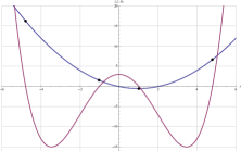
Figure 2: Graphs of the target function (blue) and constrain (red) with KKT points highlighted

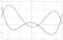
Figure 3: Comparison for the Lagrangian with positive (blue) and negative multipliers( red)

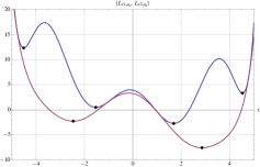
Figure 4: Augmented Lagrangian for $\mu=5$ (blue) and $\mu=20$ (red).

Figure 4 shows the Lagrangian function for positive multiplier $\mu=1$ and negative multiplier $\mu=-1$. In both cases we observe the presence of a double well. In the case of positive multiplier there are the two local minima, while in the case of negative multipliers the two local maxima can be seen.

Finally in Figure 4 two augmented Lagrangian functions are shown. The blue function has a relatively smaller value of the penalty parameter, $\nu=5$, while the red function has a big value of the penalty parameter, $\nu=20$. The small values $\nu$ produce nonconvex augmented Lagrangian, and the points corresponding to local maxima of the original problem are made into local minima by the penalty term. This produces much more difficulties in numerical computation for finding the global optimal solution.

We have already showed in section 4 that the canonical duality theory is able to find the global minimum of the Lagrangian function, and at the beginning of this section we showed that the same solution is valid if the dual problem of the augmented Lagrangian is solved with also considering $\mu$ as a variable. Now we show the results for the dual when $\mu_{k}$ is fixed, by Corollary 1 the global solution of the sub-problem can be found.

We solve the problem of the augmented Lagrangian with the same parameters of the problem in Section 4, with $\mu=1$ and $\nu=5$. The function in blue of Figure 4 is the problem we want to solve. In this case the dual is:

$$P^{d}_{\nu,\mu_{k}}(\tau,\sigma)=-\frac{c^{2}}{2\left(q+(\mu_{k}+\tau)\sigma\right)}-(\mu_{k}+\tau)\left(\frac{1}{2}\sigma^{2}+\sigma d+e\right)-\frac{\tau^{2}\nu}{2}.$$

	$x$	$\tau$	$\sigma$	${\cal L}_{\nu,\mu_{k}}(x)$	$P^{d}_{\nu,\mu_{k}}(\tau,\sigma)$	$G(\tau,\sigma)$	$(\mu+\tau)$
$(x_{1},\tau_{1},\sigma_{1})$	1.69	-0.91	-4.57	-2.74	-2.74	0.59	0.09
$(x_{2},\tau_{2},\sigma_{2})$	-1.52	-0.66	-4.84	0.48	0.48	-0.66	0.34
$(x_{3},\tau_{3},\sigma_{3})$	4.53	-1.18	0.36	3.32	3.32	1.88	-0.18
$(x_{4},\tau_{4},\sigma_{4})$	-4.50	-1.30	4.13	12.35	12.35	-0.22	-0.30
$(x_{5},\tau_{5},\sigma_{5})$	-0.12	0.59	-5.99	3.72	3.72	-8.54	1.59
$(x_{6},\tau_{6},\sigma_{6})$	-3.65	-2.96	0.65	17.38	17.38	-0.27	-1.96
$(x_{7},\tau_{7},\sigma_{7})$	3.57	-2.99	0.36	10.16	10.16	0.28	-1.99

Table 2: Critical points of the augmented Lagrangian. The first four points correspond to the KKT points of the original problem, while the last three to the to the maxima of the Lagrangian function

Table 2 lists all critical points of the primal problem and the dual problem. From these results we can see that there is no duality gap between the primal solutions and their canonical dual solutions. By the fact that the point $(x_{1},\tau_{1},\sigma_{1})$ satisfies both the conditions: $G(\tau,\sigma)\succeq 0$ and $(\mu+\tau)>0$, it is the point corresponding to the global minimum of the primal problem, just as it is reported in Corollary 1. Moreover by updating $\mu_{k+1}=\mu_{k}+\tau_{1}=0.09$ for the next iteration, the value of the multiplier gets closer to the one corresponding to the global minimum, as reported in Table 1. Furthermore, by the conditions in Remark 2 adapted for this sub-problem, the point $(x_{4},\tau_{4},\sigma_{4})$ is the biggest local maximum of the original problem.

This example shows that even if the problem with non-convex constraints becomes more complicated due to the additional penalty term, the canonical duality theory is still able to find the global solution. It is also important to note that for a problem with nonlinear constraints, the augmented Lagrangian methods usually produce a nonconvex sub-problem with double local minimizers. Traditional direct methods and algorithms for solving such highly nonconvex problems have great difficulties to find a good solution.

6 Conclusions

In this paper we have shown that the canonical duality theory presents a unified framework to cover traditional Lagrangian duality and KKT theory. For general nonlinear constrained problems, the popular penalty methods and augmented Lagrangian theory may produce nonconvex sub-problems. Theorem 5.1 shows that as long as the nonconvex constraints satisfy the conditions in Assumption 1 and 2, the canonical duality theory can be used to solve the problem and the augmented Lagrangian method is indeed not necessary.

Finally we showed that even with the unnecessary nonconvex term produced by the penalty method, the canonical duality theory is still able to find the the best solution of the problem.

References

• (1) Birgin, E.G., Castillo, R.A., MartÍnez, J.M.: ”Numerical Comparison of Augmented Lagrangian Algorithms for Nonconvex Problems”, Computational Optimization and Applications 31, 31-55 (2005).
• (2) Chen, Y. and Gao, D.Y. : Global solutions to large-scale spherical constrained quadratic minimization via canonical dual approach, to appear in Optimization Methods and Software.
• (3) Gao, D.Y.: Duality principles in nonconvex systems: Theory, methods and applications. Kluwer Academic Publishers, Dordrecht (2000)
• (4) Gao, D.Y.: Canonical dual transformation method and generalized triality theory in nonsmooth global optimization. J. Glob. Optim. 17(1/4), 127–160 (2000)
• (5) Gao, D.Y.: Canonical duality theory: theory, method, and applications in global optimization. Comput. Chem. 33, 1964–1972 (2009)
• (6) Gao, T.K.: Complete solutions to a class of eighth-order polynomial optimization problems, IMA J. Appl. Math, (2013). doi:10.1093/imamat/hxt033
• (7) Gao, D.Y., Ruan, N., Pardalos, P.M.: Canonical dual solutions to sum of fourth-order polynomials minimization problems with applications to sensor network localization. In: Pardalos, P.M., Ye, Y.Y., Boginski, V., Commander, C. (eds) Sensors: Theory, Algorithms and Applications, Springer (2010)
• (8) Gao, D.Y., Ruan, N., Sherali, H.D.: Solutions and optimality criteria for nonconvex constrained global optimization problems. J. Global Optim. 45, 473-497 (2009)
• (9) Gao, D. Y., Ruan, N., Sherali, H. D.: ”Solutions and optimality criteria for nonconvex constrained global optimization problems with connections between canonical and Lagrangian duality.” Journal of Global Optimization 45.3 473-497 (2009).
• (10) Gao, D.Y. and Sherali, H.D.: Canonical duality: Connection between nonconvex mechanics and global optimization, in Advances in Appl. Mathematics and Global Optimization, 249-316, Springer (2009).
• (11) Gao, D. Y. and Yang, Wei-Chi. Minimal distance between two non-convex surfaces. Optimization, Vol. 57, Issue 5, pp. 705-714 (2008).
• (12) Glowinski, R.: ”Augmented Lagrangian Methods: Applications to the Numerical Solution of Boundary-Value Problems”, Elsevier Science (2000).
• (13) Lagrange, Joseph-Louis: Mecanique Analytique. Courcier (1811), (reissued by Cambridge University Press, 2009; ISBN 978-1-108-00174-8).
• (14) Latorre, V., Gao, D.Y.: Canonical dual solution to nonconvex radial basis neural network optimization problem. submitted to Neurocomputing (2013)
• (15) Ruan, N., Gao, D.Y.: Global optimal solutions to a general sensor network localization problem. to appear in Perform. Eval. (2013) published online at http://arxiv.org/submit/654731
• (16) Nocedal, J., Wright, S. J.: ”Numerical Optimization (2nd edition)”. Springer (2006).
• (17) Powell, M.J.D.: ”The Lagrange method and SAO with bounds on the dual variables”, Optimization Methods and Software, (2013).
• (18) Wang, Z.B., Fang, S.C., Gao, D.Y., Xing, W.X.: Canonical dual approach to solving the maximum cut problem. J. Glob. Optim. 54, 341–352 (2012)
• (19) Zhang, J., Gao, D.Y., Yearwood, J.: A novel canonical dual computational approach for prion AGAAAAGA amyloid fibril molecular modeling. J. Theor. Biol. 284, 149–157 (2011)