Ultralong distance coupling between asymmetric resonant microcavities

Abstract

The ultralong distance coupling between two Asymmetric Resonant Microcavities (ARCs) is studied. Different from traditional short distance tunneling coupling between microcavities, the high efficient free space directional emission and excitation allow ultralong distance energy transfer between ARCs. In this paper, a novel unidirectional emission ARC, which shows directionality $I_{40}=0.54$, is designed for materials of refractive index $n=2.0$. Compared with regular whispering gallery microresonators, the coupled unidirectional emission ARCs show modulations of resonance frequency and linewidth even when the distance between cavities is much longer than wavelength. The performances and properties of the ultralong distance interaction between ARCs are analyzed and studied by coupling mode theory in details. The ultralong distance interaction between ARCs provides a new way to free-space based optical interconnects between components in integrated photonic circuits.

I Introduction

Atoms are bonded together to form molecules, which greatly enrich our world. The same story is true for microcavities 1 . Coupling of two microdisks 2 ; 3 ; 4 ; 5 provide appealing characters, such as high-Q unidirectional emission, low-threshold and single-frequency laser. These bonded microcavities, known as the photonic molecule 6 key-1 , are formed relying on the bond interaction which comes from the short distance evanescent coupling. Nevertheless, the typical length of evanescent tail of optical modes reaching out of the cavities is smaller than the wavelength, thus it is required a subtle control on subwavelength interval between cavities for forming of a designed photonic molecule. Therefore, the experiment difficulties are increased and the applications are limited.

For example, Stock et al. 7 presented recently an on-chip integrated quantum optical system made up with two micropillars: one micropillar is an electrically pumped microlaser which serves as the integrated light source, the other micropillar is a microcavity containing quantum dots which serves as quantum optical device. In this configuration, the energy transfered from the light source to the device is crucial. However, due to the fact that each pillar cavity is covered by an electrode or a micro-aperture which much larger than themselves, the gap between two cavities is naturally much longer than the wavelength, thus the short distance interaction is very inefficient. As suggested by the authors, the asymmetric resonant cavities (ARCs), instead of regular circular shaped cavities, can be applied for efficient energy transfer.

In this paper, we numerically demonstrated the ultralong distance interaction between ARCs through radiation coupling. The key issue of the long distance interaction is the high directionality emission of ARC, which determines the light emission and collection efficiency 9 ; 10 ; 11 . First of all, we proposed a novel ARC for unidirectional emission. Then, we carried out a strong far-field coupling system composed by two ARCs placed as emission direction opposite to each other. Next, numerical and theoretical studies are performed to investigate the unidirectional emission character of individual cavity, coupling induced resonance variation, and energy transferring between two cavities. The ultralong coupling scheme provides a new energy saving way to exchange energy on-chip.

II ARC with Unidirectional Emissions

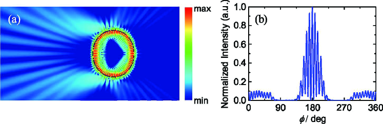
Figure 1: The near field (a) and far-field (b) distributions of $\mathrm{TM}_{37,1}$. Red-green-blue false colors indicate intensity from high to low in logarithmic scale.

Directional emission is essential for free space radiation and excitation of microcavity, so we should carefully choose a proper cavity. Here, we focus on the coupling between two cavities, thus the unidirectional emission is necessary. Different from the most design aiming on a high ($n=3.3$) 12 ; 14 or a low ($n=1.5$) 13 ; 14 refractive index, we focus on the cavity with middle refractive index around $n=2.0$ in which condition the previous cavity design is not applicable, for the relative refractive index of the semiconductor cavity embedded in polymer or silica in Ref. 7 and also refractive index of some materials, such as SiN and diamond, are near 2.0.

Based on the analysis of cavity’s symmetry, the cavity shape for high quality factor and unidirectional emission can be written as 14

$$B(\phi)=\begin{cases}R(1-{\textstyle\sum}_{i}a_{i}\cos^{i}\phi),&-\pi/2<\phi\leq\pi/2\\ R(1-{\textstyle\sum}_{i}b_{i}\cos^{i}\phi),&\pi/2<\phi\leq 3\pi/2\end{cases}$$ (1)

where $\phi$ is the polar angle respected to right direction of horizontal axis, and R is the radius . In the frame of ray optics, the boundary $B(\phi)$ of a cavity with unidirectional emission is optimized by using a hill-climbing algorithm 16-1 . We obtain a set of parameters for unidirectional emission. These are $a_{2}=0.03693$, $a_{3}=0.09501$, $b_{2}=0.09791$, $b_{3}=-0.02404$, and zero for other $a_{i}$, $b_{i}$.

Now we turn to wave optics. In the designed ARC, a transverse magnetic (TM) mode, which has only one no-zero electric field component in direction perpendicular to the cavity plane, characterized as $\mathrm{TM}_{37,1}$, which is found through boundary elements method 15 ; 16 . In the distribution of normalized intensity of this mode in logarithmic scale [Fig. 1(a)], two main emission regions lie in the top and the bottom sites. Through these sites, the radiation from the mode $\mathrm{TM}_{37,1}$ mainly propagates toward the left direction, and forms a narrow and high emission peak near the angle of $180^{\circ}$ in the far-field angular distribution (Fig. 1(b)). From the far-field distribution, it is found that 54% of total emission energy is enclosed in the angle of 40^∘ around the main peak or say technically $I_{40}=0.54$ 16-1 .

The dimensionless eigenfrequency of $\mathrm{TM}_{37,1}$ is $kR=22.32621-0.00011i$, where i stands for the imaginary unit. The imaginary part $\mathrm{Im}(kR)$ characterizes the dissipation of the cavity mode, satisfy the relation

$$\mathrm{Im}(kR)=\frac{-\mathrm{Re}(kR)}{2Q}$$ (2)

where Q is quality factor of a mode. Note that since the numerical error raised in our calculation (total boundary element number is 1600) is much larger than $\mathrm{Im}(kR)$, it is hard to solve the tiny imaginary part $\mathrm{Im}(kR)$ directly [6, 17]. In this paper, we solve the accurate Q with the help of energy flow method 18 , then obtain the $\mathrm{Im}(kR)$ through Eq. (2).

III Numerical Results about the Coupling

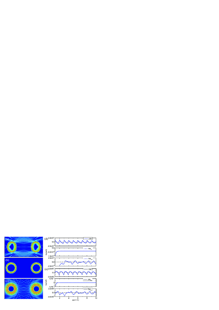
Figure 2: Far-field coupling patterns of $\mathrm{TM}_{37,1}$ (a) of the ARC, $\mathrm{TM}_{40,1}$ (b), and $\mathrm{TM}_{30,3}$ (c) of circular cavity. The real (d) and imaginary (e) parts of $\Delta kRs$ vary with gap L between two cavities.

Place two aforementioned ARCs together with mirror symmetry about the vertical axis, and let their main emission directions pointing to each other to form a double-cavities system. Since the system is linear, we can deduce the dynamics of ARCs through the eigenmodes of the system. Therefore, we resort eigenvalue equation to investigate this system rather than research the complicated dynamic process of coupling directly. When the gap L (Fig. 3) between the cavities is 3R, an intensity distribution of the eigenmode, whose resonant frequency $kR_{\mathrm{EE}}=22.32617-0.00011i$ corresponding to $\mathrm{TM}_{37,1}$ in single ARC, of the system is calculated by solving the eigenfunction of $kR$ (Fig. 2(a)) 16 . As we can see in the figure, intensity along the vertical and horizontal axis of symmetry is maximum, so corresponding complex amplitude distribution of optical field has reflective symmetry about the two axes. This mode is classified as even-even (EE) mode. Near the resonant frequency of EE mode, there always exist other three classes of mode (odd-even, even-odd, and odd-odd) in the weak coupling system with four-fold reflective symmetry. In our classification, the first and last symmetry indicators (E or O) refer to symmetry state about vertical and horizontal axis, respectively. In Fig. 2(a), obvious interference fringes with regular periodic oscillation are shown outside the cavities. Furthermore, the interference fringes inside the cavities are different to single cavity pattern either (Fig. 1(a)).

To compare with coupling of circular cavities without directional emission, two EE modes in coupled circular cavities are calculated with parameters: gap $L=3R$, radius $R=1$, refractive index $n=2.0$. The $\mathrm{TM}_{40,1}$ and the $\mathrm{TM}_{30,3}$ modes are found around $kR=22.3$ with $kR_{c1}=22.70596-5.7\times 10^{-13}i$ and $kR_{c3}=22.02345-0.00004i$, respectively. Because the Q of $\mathrm{TM}_{40,1}$ mode is as high as $2.0\times 10^{13}$, in other words, little energy can leak out from the cavities. Intensity outside the cavities is failed to be depicted even in logarithmic coordinates (Fig. 2(b)). In this case, the coupling between the modes of two cavities can be ignored, and the field distribution and the resonant frequency consisted with that of the isolated cavity. For the $\mathrm{TM}_{30,3}$ mode, its $Q\sim 2.5\times 10^{5}$ is much less than that of $\mathrm{TM}_{40,1}$ mode, while it is in the same order of magnitude with the $Q\sim 1.0\times 10^{5}$ of $\mathrm{TM}_{37,1}$ mode of coupled ARCs. At this point, a regular intensity lattice between the two cavities is formed by interference. Moreover, the distribution of the regular pattern is consistent with the interference field between the emissions of two isolated cavity modes.

Further more, by changing the gap L between the two cavities, we investigate how the resonant frequency of the three EE modes varies with L. In this paper, we only concern the long distance radiation coupling instead of near distance tunneling coupling, so the case of $L<\lambda$, which has been well investigated in many studies of optical molecular, is omitted. Figures 2(d) and (e) show the real and imaginary part of the kR relative to the isolated one of three modes varying with $L\in\left[\lambda,10\lambda\right]$, respectively.

The $\mathrm{Re}(\Delta kR)$ and $\mathrm{Im}(\Delta kR)$ of $\mathrm{TM}_{37,1}$ mode of coupled ARCs vary periodically with L, and the variation period is $\lambda$. It suggests that an efficient coupling channel is established between the ARCs. In addition, the maximum value of the $\mathrm{Re}(\Delta kR)$ curve shift left about $\lambda/4$ to the $\mathrm{Im}(\Delta kR)$ curve. Their variation amplitudes are the same in magnitude of $10^{-4}$ at $L=\lambda$, and decrease slowly as increasing of L. Besides, the variation is around resonant frequency $kR=22.32621-0.00011i$ of isolated cavity, and the limited frequency at $L=\infty$ tend to the frequency of isolated cavity also. All above is in line with physical expectations.

Now, we turn to the variation of resonant frequency of coupled circular cavities. The $\mathrm{Re}(\Delta kR)$ of $\mathrm{TM}_{40,1}$ mode does not show any oscillation in the order of $10^{-6}$, when the L is larger than $1.5\lambda$. As to its $\mathrm{Im}(\Delta kR)$, the no oscillation order is down to $10^{-11}$. The oscillation of resonant frequency of $\mathrm{TM}_{30,3}$ mode is irregular. The amplitude of oscillation is about $10^{-5}$, an order of magnitude less than that of ARC case.

The oscillation amplitude positively associated with the coupling strength between the two cavities, even count the ratio of Qs of$\mathrm{TM}_{30,3}$ to $\mathrm{TM}_{37,1}$, the coupling strength is enhanced four times in coupled ARCs. We can draw a conclusion safely that the coupling strength and stability of ARCs are both better than that of circular cavities because of the character of the unidirectional emission.

IV Analysis by the Coupled-Mode Theory

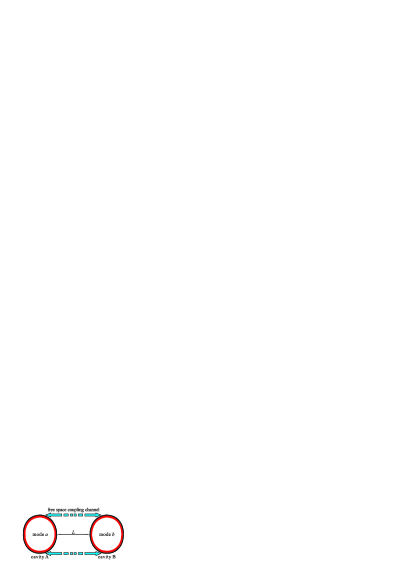
Figure 3: Schematics of coupled cavities.

Based on the image of the long distance coupling between ARCs in Fig. 2(a), we can establish a simple model of radiation coupled cavities [see Fig. 3]. The eigenmode of separated ARC is described by the wave function $\Psi_{a(b)}(r)$, with the frequency and intrinsic loss of $\omega_{a(b)}=\mathrm{Re}(k_{a(b)})\times c$ and $\kappa_{a(b)}=-\mathrm{Im}(k_{a(b)})\times c$, where c is the speed of light in vacuum. For isolated ARCs, the dynamics of cavity field can be expressed as $\Phi_{a}(r,t)=a(t)\Psi_{a}(r)=a(0)e^{(-i\omega_{a}-\kappa_{a})t}\Psi_{a}(r)$ and $\Phi_{b}(r,t)=b(t)\Psi_{b}(r)=b(0)e^{(-i\omega_{b}-\kappa_{b})t}\Psi_{b}(r)$, with dimensionless coefficients of $a(t)$ and $b(t)$ .

With weak coupling perturbation, the wave function of a composite system can be written as $\Phi(r,t)=a(t)\Psi_{a}(r)+b(t)\Psi_{b}(r)$ 19 . Considering the radiation coupling between two ARCs, and according to the coupled-mode theory, the dynamics of the system satisfy the following differential equations

$$\begin{cases}\frac{d}{dt}a(t)=(-i\omega_{a}-\kappa_{a})a(t)+ge^{i\theta}b(t)\\ \frac{d}{dt}b(t)=(-i\omega_{b}-\kappa_{b})b(t)+ge^{i\theta}a(t)\end{cases}$$ (3)

where $ge^{i\theta}$ is the term of radiation coupling , in which $g\geq 0$ is the coupling strength and $\theta$ is the phase shift that the coupling wave undergoes from a cavity to another.

According to the coupled mode equations, we can solve the new normal modes of the composite system as $\Psi_{\pm}(r)=c_{a}\Psi_{a}(r)+c_{b}\Psi_{b}(r)$, which frequency $\omega_{\pm}$ and coefficients $\left(\begin{array}[]{c}c_{a}\\ c_{b}\end{array}\right)$ are just the eigenvalues and eigenvectors of the matrix

$$M=\left(\begin{array}[]{cc}\omega_{1}&\gamma\\ \gamma&\omega_{2}\end{array}\right)=\left(\begin{array}[]{cc}-i\omega_{a}-\kappa_{a}&ge^{i\theta}\\ ge^{i\theta}&-i\omega_{b}-\kappa_{b}\end{array}\right).$$ (4)

It is easy to solve the eigenfrequency

$$\omega_{\pm}=\frac{1}{2}(\omega_{1}+\omega_{2}\pm\sqrt{(\omega_{1}-\omega_{2})^{2}+4\gamma^{2}}),$$ (5)

and corresponding coefficients

$$\left(\begin{array}[]{c}c_{a}\\ c_{b}\end{array}\right)=\frac{1}{\sqrt{|\omega_{\pm}-\omega_{1}|^{2}+|\gamma|^{2}}}\left(\begin{array}[]{c}\gamma\\ \omega_{\pm}-\omega_{1}\end{array}\right).$$ (6)

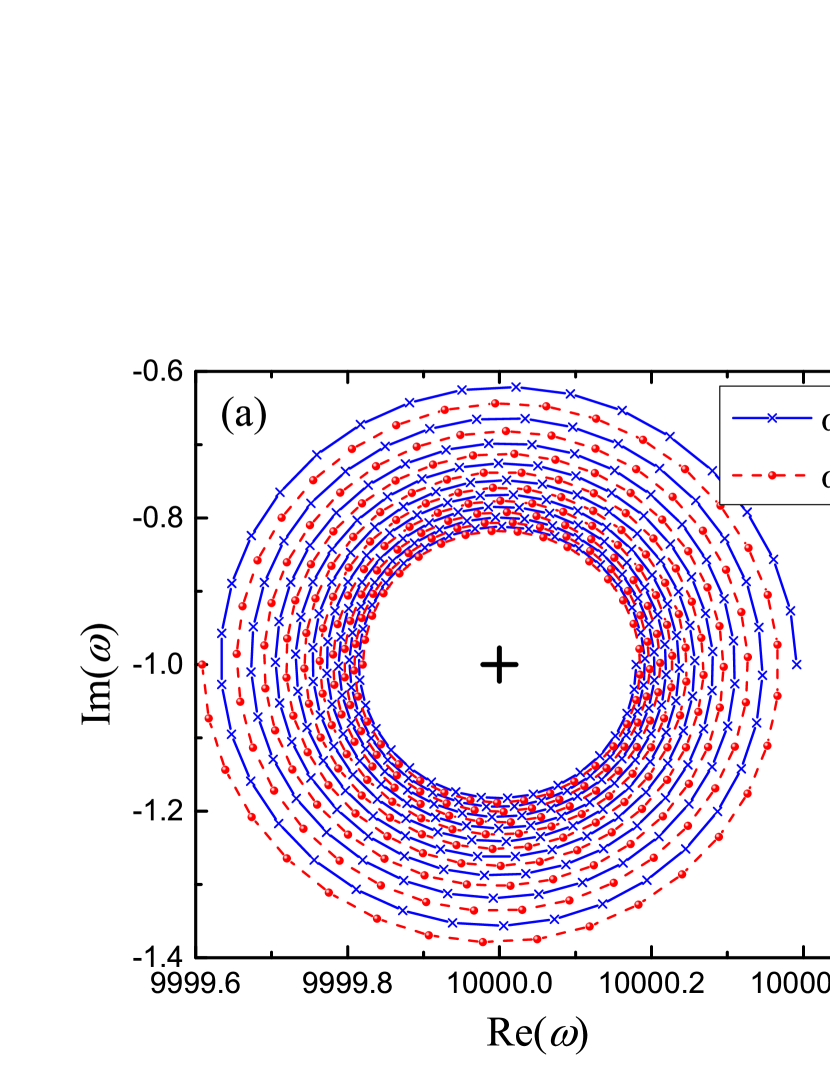
Figure 4: The tracks of kR theory (a) and simulation (b). Center cross indicate the location of resonant frequency without coupling.

For example, in the case of two identical ARCs, i.e. $\omega_{a}=\omega_{b}$ and $\kappa_{a}=\kappa_{b}$, we have $\omega_{\pm}=-i\omega_{a}-\kappa_{a}\pm ge^{i\theta}$ and $\Psi_{\pm}=\frac{1}{\sqrt{2}}(\Psi_{a}\pm\Psi_{b})$. To the radiation coupling, the phase $\theta$ is proportional to the propagation distance L as $\theta=\frac{L}{\lambda}\times 2\pi+\theta_{0}$, where $\theta_{0}$ is constant phase according to coupling phase when $L=0$. Therefore, when the $\theta$ increases with the increasing of L, the points of $\omega_{\pm}$ draw a circle centered at $\omega_{1}$ and with radius g in the complex plan of $\omega$. Noting that a pair of $\omega_{+}$ and $\omega_{-}$ always locate at the ends of a diameter of the circle. Additionally, g is not a constant but a function of L. Since g stands for the magnitude of coupling, i.e. a portion of emitting energy from one cavity coupled into the other cavity, we can assume the function as

$$g(L)=g(0)/\sqrt{L+2R}.$$ (7)

The magnitude of g must less than that of $\mathrm{Im}(\omega_{1})$, which refers to the emission amount of one cavity. Consequently, the data range of g is $[0,1]\times\mathrm{Im}(\omega_{1})$. Let us give an example. Assuming $\theta_{0}=0$, $\lambda=0.3$, $g(0)=0.9$, and $L\in[1,10]\times\lambda$, we get the double spiral curves of $\omega_{\pm}$ in $\omega$ plane (Fig. 4(a)), which starts from the outer points and gradually approaches the center cross $\omega_{1}$ with increasing of L.

The $\omega_{+}$ is associated with k, which is calculated in the last section, with proportional relationship $\omega_{+}=-ikc$. Transporting the curves of ARCs in Fig. 2 to a spiral curve in kR complex plane, we get the kR track of varying with L (Fig. 4(b) blue solid line). The point on the spiral curve closes to center cross with increasing L, which indicates that the coupling strength is not a constant but a decreasing value too. In addition, the density of points in upper part of the curve is higher than that in the under part. It reveals that there is no strictly linear relationship between the $\theta$ and the L. Furthermore, a kR track of odd-even mode corresponding to $\omega_{-}$ is calculated (Fig. 4(b) red dash line). Again, it is a spiral curve like the track of EE mode, and intertwined with the spiral line of EE mode around the center cross.

Though the pictures of analytical and numerical results are qualitatively consistent with each other, the last one is more complicated. The reason is the real coupling term $ge^{i\theta}$ as a function of L is more complex than we assumed. For example, not like the waveguide coupling case, in free space coupling case, coupling phase $\theta$ is related with the shape and location of the beam emitted by isolated cavity. So, the linear relationship with L is a simplified model.

Before a further discussion, we evaluate the $g$ from the data shown in Fig. 4(b), for $2g=|\omega_{+}-\omega_{-}|$. As is shown in Fig. 5(a) (solid blue line), when the L increases the envelope of $g$ decreases slowly. Obviously, a relatively high $g$ ($>0.4$) last in a wide range to $L=10\lambda$. Besides, a fitted line (Fig. 5(a) dash red line) according to Eq. (7) agrees with simulation data in certain degree, if we ignore the oscillation. Here, the oscillation stems from multi-modes combination induced by multi-channel coupling in free space 11 , which is not included in our simplified model of single mode coupling.

V Dynamics of Coupled ARCs

V.1 On-resonance

Since the eigenfunction $\Phi_{\pm}$ of coupled mode is known, the time evolution of any complex function $\Phi$ in the subspace can be determined. Here, as an example, we set the initial state of coupled system to $\Phi_{a}$, and discuss the energy transportation between the two coupled cavities.

When $t=0$, we have $\Phi(r,0)=\Phi_{a}(r,0)=[\Phi_{+}(r,0)+\Phi_{-}(r,0)]/\sqrt{2}$. Later the state function at time t reads

$$\Phi(r,t) =\frac{1}{\sqrt{2}}[\Phi_{+}(r,0)e^{\omega_{+}t}+\Phi_{-}(r,0)e^{\omega_{-}t}]$$ (8)

To find the energy in the two cavities, last formula can be rewritten as:

$$\Phi(r,t) =\frac{1}{2}[(e^{\omega_{+}t}+e^{\omega_{-}t})\Psi_{a}+(e^{\omega_{+}t}-e^{\omega_{-}t})\Psi_{b}]$$ (9)

The normalized energy in cavity A or B reads

$$E_{a,b} =\left|\frac{1}{2}(e^{\omega_{+}t}\pm e^{\omega_{-}t})\right|^{2}$$

$$=\frac{1}{2}e^{-2\kappa_{a}t}[\cosh(2g\cos\theta\cdot t)\pm\cos(2g\sin\theta\cdot t)]$$ (10)

where positive and negative sign correspond to a and b, respectively.

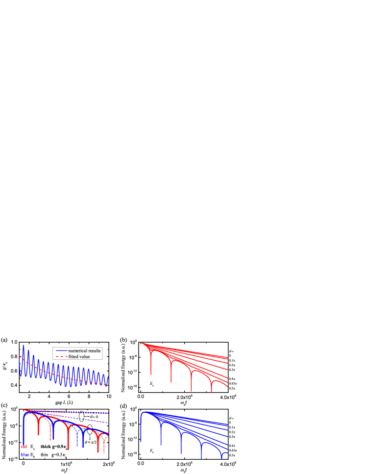
Figure 5: (a) The values of $g/\kappa_{a}$ get from simulation results (solid blue line) and Eq. (7) with $g(0)=1.4$ (dash red line). Time evolution of normalized energy of two coupled cavities. Energy in cavity A (b) and B (d) vary with time when $g=0.68\kappa_{a}$ and $\theta=0,\,0.1\pi,\,0.2\pi,\,0.3\pi,\,0.4\pi,\,0.45\pi,\,0.5\pi$. (c) Evolution of energy at different combination of parameters.

Taking some examples, the mode $\mathrm{TM}_{37,1}$ in isolated ARC has a $Q\sim 10^{5}$, i.e. $\kappa_{a}=5\times 10^{-6}\omega_{a}$. We pick a middle $g=0.68\kappa_{a}$ and observe the time evolution of energy in cavity A and B at some coupling angles of $\theta$(Figs. 5(b) and (d)). When $\theta=0$, the curves show there is already considerable energy transported from cavity A into cavity B at the time $\omega_{a}t\sim 2.5\times 10^{5}$, though the initial energy is wholly in cavity A. Then after a period of time the energy is balanced in both cavity, and attenuates exponentially with slope of $-2(\kappa_{a}-g)/\omega_{a}$. Enlarge the $\theta$ gradually, the feature of transportation of energy is similar with case of $\theta=0$ except the final attenuation slope which changes to $-2(\kappa_{a}-g\cos\theta)/\omega_{a}$. When the $\theta$ close to $\pi/2$, such as $0.45\pi$, the augment $2g\cos\theta\cdot t$ of attenuation (first) term bracketed in Eq. (10) is small, while the oscillating (second) term plays a major role when t is not too large. At this time, energy oscillates between the two cavities several times, then the amplitude of the oscillation reduces to zero, and energy becomes equal in two cavities. When the $\theta$ equals $\pi/2$, only the oscillating term left in square bracket of Eq. (10). Thus, energy attenuates with oscillation (Fig. 5 solid line), that is to say the energy in the two cavities empty in turn. The attenuation slope reach the maxima value $-2\kappa_{a}/\omega_{a}$. The case of $\theta\in[\pi/2,\pi]$ repeats the result in interval $[0,\pi/2]$ with the reversal manner $\pi-\theta$. Furthermore, $\pi$ is the period of the dynamic rule of the evolution of modes varying with $\theta$.

Then we change the $g$ to $0.5\kappa_{a}$ and $0.9\kappa_{a}$ for comparison (Fig. 5(c)). To the smaller $g=0.5\kappa_{a}$ case, the speed of energy exchange slows down, and the time requirement for energy balance in coupled cavities increases. Moreover, the proportion of the energy transported from one cavity to another decreases, i.e. more energy emits out of the coupling system. Hence, the slope of energy attenuation line decreases except the constant slope in $\theta=\pi/2$ case. If $\theta=\pi/2$, the period of energy emptying in cavities increases with decreasing of g. On the contrary, if we change the mode used in coupling with different Q, then the time to achieve energy balance is proportional to the Q.

V.2 Off-resonance

Figure 6: Time evolution of normalized energy of two mismatched cavities. Three columns, from left to right, week, middle, and strong represent detuning, respectively. Each row cope with a typical value of $\theta$. Insert in (c): middle detuning and with $\theta=0.75\pi$.

In practice, two coupled cavities may not be identical but have slight different geometry, so the resonant frequencies of cavities have a small mismatch, i.e. $\omega_{1}\neq\omega_{2}$. Keeping $\kappa_{a}$ and $\kappa_{b}$ equal, we study the detuning $\delta=\omega_{a}-\omega_{b}$ influence on the dynamics of the coupling. Then, like in the on-resonance case, after derivation from Eq. (6) we get the evolution equation of energy and depict it in Fig. 6 with $g=0.68\kappa_{a}$ and $Q=10^{5}$ again.

If the detuning induced by size difference is slight, say $\delta=0.1\kappa_{a}$, the resonances in two cavities overlap significantly with each other. Then, the resonant frequency of coupled mode still varies around the average value of isolated frequencies. Yet the reduction of the coupling strength shrinks the splitting of two coupled modes. Besides, energy of modes distribute unequally in two cavities after a transient state. When $\theta$ increases from 0 to $0.5\pi$, the unbalance of the energy distribution becomes worse and the slope of the decay curve becomes steeper (Fig. 6 first and second columns). For the Fig. 6(c), though the cavity A keep more energy than cavity B in the oscillation, the oscillation period is nearly as same as that in on-resonance case (Fig. 5(c) thin line).

The imbalance of energy distribution becomes more serious when the detuning $\delta$ gets larger. In the middle detuning case $\delta=1\kappa_{a}$ (Fig. 6 second column), we found whether the over coupling or under coupling occurs depends on the coupling phase $\theta$. For instance, when $\theta=0.25\pi$ the energy flow from cavity A to cavity B can not reflow back to cavity A completely, but when $\theta=0.75\pi$ the energy in cavity A can not transport to B entirely (Fig. 6 middle panel and its insert). In addition, the evolution of energy about the $\theta$ is also in the period of $\pi$ but is different in the cases of $\theta$ with of $\pi-\theta$ .

In fact, when the detuning is much larger than the linewidth, say $\delta\gg\kappa_{a}$, the resonated mode in one cavity is merely influenced by another cavity (Fig. 6 last column). In other words, energy cannot deliver from cavity A to cavity B efficiently, so mode a decays exponentially without oscillation. At this time, a very few energy in cavity B oscillates intensely, as there arises a beat oscillation, whose period is inversely proportional to $\delta$.

VI Conclusion

In summary, an efficient coupling in long distance is established by employing unidirectional ARCs. We designed a unidirectional cavity with refractive index 2.0 for coupling. Comparing with the free-space far-field coupling of two circular cavities, the coupling of ARCs is strong and stable, which makes ARC being the first choice for far-field coupling. The coupled mode theory works well on solving the coupled problem based on the isolated mode. Results show that the coupled mode is the superposition of two single modes, and the corresponding resonant frequency is the sum (difference) of single mode frequency and a coupling term. Moreover, based one the result of the coupled mode theory, the time revolution of the light field, which is described by an arbitrary complex function, can be calculated by decomposing it with bases of normal mode. Then under on- and off-resonance coupling conditions, the transmission of energy in the coupling system is depicted in time domain. It need to note that coupling mode or time domain characters both extremely rely on the coupling phase $\theta$. So far we have solved the low coupling efficiency problem encountered in Ref. 7 .This paper only discusses two coupled passive ARCs. Next, coupling system composed of a laser cavity and a passive cavity 8 in ARC form need to be studied, and the coupling of multi-cavities key-2 is interesting too.

References

- (1) K. J. Vahala, “Optical microcavties,” Nature 424, 839-846 (2003).
- (2)
- (3)
- (4) J.-W. Ryu, S.-Y. Lee, C.-M. Kim, and Y.-J. Park, “Directional interacting whispering-gallery modes in coupled dielectric microdisks,” Phys. Rev. A 74, 013804 (2006).
- (5)
- (6)
- (7) J. J. Li, J. X. Wang, and Y. Z. Huang, “Mode coupling between first-and second-order whispering-gallery modes in coupled microdisks,” Opt. Lett. 32, 1563-1565 (2007).
- (8)
- (9)
- (10) J. W. Ryu, and M. Hentschel, “Designing coupled microcavity lasers for high-Q modes with unidirectional light emission,” Opt. Lett. 36, 1116-1118 (2011).
- (11)
- (12)
- (13) X. Tu, X. Wu, L. Liu, and L. Xu, “High-Q unidirectional emission properties of the,” J. Opt. Soc. Am. B 27, 300-304 (2010).
- (14)
- (15) Y. P. Rakovich, and J. F. Donegan, “Photonic atoms and molecules,” Laser Photonics Rev. 4, 179-191 (2009).
- (16) T. Grossmann, T. Wienhold, U. Bog, T. Beck, C. Friedmann, H. Kalt, and T. Mappes, “Polymeric photonic molecule super-mode lasers on silicon,” Light: Sci. & Appl. 2, e82 (2013).
- (17) E. Stock, F. Albert, C. Hopfmann, M. Lermer, C. Schneider, S. H fling, A. Forchel, M. Kamp, and S. Reitzenstein, “On-chip quantum optics with quantum dot microcavities,” Adv. Mater. 25, 707-710 (2013).
- (18) E. I. Smotrova, and A. I. Nosich, “Optical coupling of an active microdisk to a passive one: effect on the lasing thresholds of the whispering-gallery supermodes,” Opt. Lett. 38, 2059-2061 (2013).
- (19) S.-B. Lee, J. Yang, S. Moon, J.-H. Lee, and K. An, “Chaos-assisted nonresonant optical pumping of quadrupole-deformed microlasers,” Appl. Phys. Lett. 90, 041106 (2007).
- (20) F.-J. Shu, C.-L. Zou, and a. F.-W. Sun, “Dynamic process of free space excitation of asymmetric resonant microcavity,” J. Lightwave Technol. 31, 1884-1889 (2013).
- (21) C.-L. Zou, F.-J. Shu, F.-W. Sun, Z.-J. Gong, Z.-F. Han, and G.-C. Guo, “Theory of free space coupling to high-Q whispering gallery modes,” Opt. Express 21, 9982-9995 (2013).
- (22) J. Wiersig, and M. Hentschel, “Combining directional light output and ultralow loss in deformed microdisks,” Phys. Rev. Lett. 100, 033901 (2008).
- (23) X. F. Jiang, Y. F. Xiao, C. L. Zou, L. He, C. H. Dong, B. B. Li, Y. Li, F. W. Sun, L. Yang, and Q. Gong, “Highly unidirectional emission and ultralow-threshold lasing from on-chip ultrahigh-Q microcavities,” Adv. Mater. 24, OP260-OP264 (2012).
- (24) C.-L. Zou, F.-W. Sun, C.-H. Dong, F.-J. Shu, X.-W. Wu, J.-M. Cui, Y. Yang, Z.-F. Han, and G.-C. Guo, “High Q and unidirectional emission whispering gallery modes: principles and design,” IEEE J. Sel. Top. Quantum Electron. 19, 9000406 (2013).
- (25) F.-J. Shu, C.-L. Zou, and F.-W. Sun, “An optimization method of asymmetric resonant cavities for unidirectional emission,” J. Lightwave Technol. 31, 2994-2998 (2013).
- (26) J. Wiersig, “Boundary element method for resonances in dielectric microcavities,” J. Opt. A: Pure. Appl. Opt. 5, 53-60 (2003).
- (27) C. L. Zou, H. G. L. Schwefel, F. W. Sun, Z. F. Han, and G. C. Guo, “Quick root searching method for resonances of dielectric optical microcavities with the boundary element method,” Opt. Express 19, 15669-15678 (2011).
- (28) C.-L. Zou, Y. Yang, C.-H. Dong, Y.-F. Xiao, Z.-F. Han, and G.-C. Guo, “Accurately calculating high quality factor of whispering-gallery modes with boundary element method,” J. Opt. Soc. Am. B 26, 2050-2053 (2009).
- (29) H. A. Haus, and W. Huang, “Coupled-mode theory,” Proc. IEEE 79, 1505-1518 (1991).
- (30) M. D. Weed, C. G. Williams, P. J. Delfyett, and W. V. Schoenfeld, “Symmetry Considerations for Closed Loop Photonic Crystal Coupled Resonators,” J. Lightwave Technol. 31, 1426-1432 (2013).