Statistical Estimation and Testing via the Sorted $\ell_{1}$ Norm

Abstract

We introduce a novel method for sparse regression and variable selection, which is inspired by modern ideas in multiple testing. Imagine we have observations from the linear model $y=X\beta+z$, then we suggest estimating the regression coefficients by means of a new estimator called SLOPE, which is the solution to

$$\underset{b}{\text{minimize}}\quad{\textstyle\frac{1}{2}}\|y-Xb\|_{\ell_{2}}^{2}+\lambda_{1}|b|_{(1)}+\lambda_{2}|b|_{(2)}+\ldots+\lambda_{p}|b|_{(p)};$$

here, $\lambda_{1}\geq\lambda_{2}\geq\ldots\geq\lambda_{p}$ and $|b|_{(1)}\geq|b|_{(2)}\geq\ldots\geq|b|_{(p)}$ is the order statistics of the magnitudes of $b$. In short, the regularizer is a sorted $\ell_{1}$ norm which penalizes the regression coefficients according to their rank: the higher the rank—the closer to the top—the larger the penalty. This is similar to the famous Benjamini-Hochberg procedure (BHq) [9], which compares the value of a test statistic taken from a family to a critical threshold that depends on its rank in the family. SLOPE is a convex program and we demonstrate an efficient algorithm for computing the solution. We prove that for orthogonal designs with $p$ variables, taking $\lambda_{i}=F^{-1}(1-q_{i})$ ($F$ is the cumulative distribution function of the errors), $q_{i}=iq/(2p)$, controls the false discovery rate (FDR) for variable selection. This holds under the assumption that the errors are i.i.d. symmetric and continuous random variables. When the design matrix is nonorthogonal there are inherent limitations on the FDR level and the power which can be obtained with model selection methods based on $\ell_{1}$-like penalties. However, whenever the columns of the design matrix are not strongly correlated, we demonstrate empirically that it is possible to select the parameters $\lambda_{i}$ as to obtain FDR control at a reasonable level as long as the number of nonzero coefficients is not too large. At the same time, the procedure exhibits increased power over the lasso, which treats all coefficients equally. The paper illustrates further estimation properties of the new selection rule through comprehensive simulation studies.

^a Departments of Mathematics and Computer Science, Wrocław University of Technology and Jan Długosz University, Poland
^b IBM T.J. Watson Research Center, Yorktown Heights, NY 10598, U.S.A.
^c Department of Statistics, Stanford University, Stanford, CA 94305, U.S.A.
^d Department of Mathematics, Stanford University, Stanford, CA 94305, U.S.A.

October 2013

Keywords. Sparse regression, variable selection, false discovery rate, lasso, sorted $\ell_{1}$ penalized estimation (SLOPE), prox operator.

1 Introduction

1.1 The model selection problem

This paper is concerned with estimation and/or testing in the (high-dimensional) statistical linear model in which we observe

$$y=X\beta+z;$$ (1.1)

as usual, $y\in\mathbb{R}^{n}$ is the vector of responses, $X\in\mathbb{R}^{n\times p}$ is the design matrix, $\beta\in\mathbb{R}^{p}$ is the unknown parameter of interest, and $z\in\mathbb{R}^{n}$ is a vector of stochastic errors (unless specified otherwise, we shall assume that the errors are i.i.d. zero-mean normal variables). In an estimation problem, we typically wish to predict the response variable as accurately as possible or to estimate the parameter $\beta$ as best as we can. In the testing problem, the usual goal is to identify those variables for which the corresponding regression coefficient is nonzero. In the spirit of the recent wave of works on multiple testing where we collect many measurements on a single unit, we may have reasons to believe that only a small fraction of the many variables in the study are associated with the response. That is to say, we have few effects of interest in a sea of mostly irrelevant variables.

Such problems are known under the name of model selection and have been the subject of considerable studies since the linear model has been in widespread use. Canonical model selection procedures find estimates $\hat{\beta}$ by solving

$$\min_{b\in\mathbb{R}^{p}}\,\|y-Xb\|_{\ell_{2}}^{2}+\lambda\|b\|_{\ell_{0}},$$ (1.2)

where $\|b\|_{\ell_{0}}$ is the number of nonzero components in $b$. The idea behind such procedures is of course to achieve the best possible trade-off between the goodness of fit and the number of variables included in the model. Popular selection procedures such as AIC and $C_{p}$ [4, 28] are of this form: when the errors are i.i.d. $\mathcal{N}(0,\sigma^{2})$, AIC and $C_{p}$ take $\lambda=2\sigma^{2}$. In the high-dimensional regime, such a choice typically leads to including very many irrelevant variables in the model yielding rather poor predictive power in sparse settings (when the true regression coefficient sequence is sparse). In part to remedy this problem, Foster and George [23] developed the risk inflation criterion (RIC) in a breakthrough paper. They proposed using a larger value of $\lambda$ effectively proportional to $2\sigma^{2}\log p$, where we recall that $p$ is the total number of variables in the study. Under orthogonal designs, it can be shown that this yields control of the familywise error rate (FWER); that is to say, the probability of including a single irrelevant variable is very low. Unfortunately, this procedure is also rather conservative (it is similar to a Bonferroni-style procedure in multiple testing) and RIC may not have much power in detecting those variables with nonvanishing regression coefficients unless they are very large.

The above dichotomy has been recognized for some time now and several researchers have proposed more adaptive strategies. One frequently discussed idea in the literature is to let the parameter $\lambda$ in (1.2) decrease as the number of included variables increases. For instance, penalties with appealing information- and decision-theoretic properties are roughly of the form

$$P(b)=p(\|b\|_{\ell_{0}}),\quad p(k)=2\sigma^{2}k\log(p/k)$$ (1.3)

(the fitted coefficients minimize the residual sum of squares (RSS) plus the penalty) or with

$$p(k)=2\sigma^{2}\sum_{1\leq j\leq k}\log(p/j).$$ (1.4)

Among others, we refer the interested reader to [24, 11] and to [36] for a related approach. When $\|b\|_{\ell_{0}}=1$, these penalties are similar to RIC but become more liberal as the fitted coefficients become denser.

The problem with the selection strategies above is that they are computationally intractable. Solving (1.2) or the variations (1.3)–(1.4) would involve a brute-force search essentially requiring to fit least-squares estimates for all possible subsets of variables. This is not practical for even moderate values of $p$—for $p>60$, say—and is the main reason why computationally manageable alternatives have attracted considerable attention in applied and theoretical communities. In statistics, the most popular alternative is by and large the lasso [35], which operates by substituting the nonconvex $\ell_{0}$ norm by the $\ell_{1}$ norm—its convex surrogate—yielding

$$\min_{b\in\mathbb{R}^{p}}\,{\textstyle\frac{1}{2}}\|y-Xb\|^{2}_{\ell_{2}}+\lambda\,\|b\|_{\ell_{1}}.$$ (1.5)

We have the same dichotomy as before: on the one hand, if the selected value of $\lambda$ is too small, then the lasso would select very many irrelevant variables (thus compromising its predicting performance). On the other hand, a large value of $\lambda$ would yield little power as well as a large bias.

1.2 The sorted $\ell_{1}$ norm

This paper introduces a new variable selection procedure, which is computationally tractable and adaptive in the sense that the ‘effective penalization’ is adaptive to the sparsity level (the number of nonzero coefficients in $\beta\in\mathbb{R}^{p}$). This method relies on the sorted $\ell_{1}$ norm: letting $\lambda$ be a nonincreasing sequence of nonnegative scalars,

$$\lambda_{1}\geq\lambda_{2}\geq\ldots\geq\lambda_{p}\geq 0,$$ (1.6)

with $\lambda_{1}>0$, we define the sorted $\ell_{1}$ norm of a vector $b\in\mathbb{R}^{p}$ as

$$J_{\lambda}(b)=\lambda_{1}|b|_{(1)}+\lambda_{2}|b|_{(2)}+\ldots+\lambda_{p}|b|_{(p)}.$$ (1.7)

Here, $|b|_{(1)}\geq|b|_{(2)}\geq\ldots\geq|b|_{(p)}$ is the order statistic of the magnitudes of $b$, namely, the absolute values ranked in decreasing order. For instance, if $b=(-2.1,-0.5,3.2)$, we would have $|b|_{(1)}=3.2$, $|b|_{(2)}=2.1$ and $|b|_{(3)}=0.5$. Expressed differently, the sorted $\ell_{1}$ norm of $b$ is thus $\lambda_{1}$ times the largest entry of $b$ (in magnitude), plus $\lambda_{2}$ times the second largest entry, plus $\lambda_{3}$ times the third largest entry, and so on. As the name suggests, $J_{\lambda}(\cdot)$ is a norm and is, therefore, convex.

Proposition 1.1.

The functional $\eqref{eq:orderedl1}$ is a norm provided (1.6) holds and $\lambda\neq 0$. In fact, the sorted $\ell_{1}$ norm can be characterized as

$$J_{\lambda}(b)=\sup_{w\in C_{\lambda}}\langle w,b\rangle,$$ (1.8)

where $w$ is in the convex set $C_{\lambda}$ if and only if for all $i=1,\ldots,p$,

$$\sum_{j\leq i}|w|_{(j)}\leq\sum_{j\leq i}\lambda_{j}.$$ (1.9)

The proof of this proposition is in the Appendix. For now, observe that $C_{\lambda}=\cap_{i=1}^{p}C^{(i)}_{\lambda}$, where

$$C^{(i)}_{\lambda}=\Bigl{\{}w:f_{i}(w)\leq\sum_{j\leq i}\lambda_{j}\Bigr{\}},\qquad f_{i}(w)=\sum_{j\leq i}|w|_{(j)}.$$

For each $i$, $f_{i}$ is convex so that $C^{(i)}_{\lambda}$ is convex. Hence, $C_{\lambda}$ is the intersection of convex sets and is, therefore, convex. The convexity of $f_{i}$ follows from its representation as a supremum of linear functions, namely,

$$f_{i}(w)=\sup\,\,\langle z,w\rangle,$$

where the supremum is over all $z$ obeying $\|z\|_{\ell_{0}}\leq i$ and $\|z\|_{\ell_{\infty}}\leq 1$ (the supremum of convex functions is convex [14]). In summary, the characterization via (1.8)–(1.9) asserts that $J_{\lambda}(\cdot)$ is a norm and that $C_{\lambda}$ is the unit ball of its dual norm.

1.3 SLOPE

The idea is to use the sorted $\ell_{1}$ norm for variable selection and in particular, we suggest a penalized estimator of the form

$$\min_{b\in\mathbb{R}^{p}}\,{\textstyle\frac{1}{2}}\|y-Xb\|_{\ell_{2}}^{2}+\sum_{i=1}^{p}\lambda_{i}|b|_{(i)}.$$ (1.10)

We call this Sorted L-One Penalized Estimation (SLOPE). SLOPE is convex and, hence, tractable. As a matter of fact, we shall see in Section 2 that the computational cost for solving this problem is roughly the same as that for solving the plain lasso. This formulation is rather different from the lasso, however, and achieves the adaptivity we discussed earlier: indeed, because the $\lambda_{i}$’s are decreasing or sloping down, we see that the cost of including new variables decreases as more variables are added to the model.

1.4 Connection with the Benjamini-Hochberg procedure

Our methodology is inspired by the Benjamini-Hochberg (BHq) procedure for controlling the false discovery rate (FDR) in multiple testing [9]. To make this connection explicit, suppose we are in the orthogonal design in which the columns of $X$ have unit norm and are perpendicular to each other (note that this implies $p\leq n$). Suppose further that the errors in (1.1) are i.i.d. $\mathcal{N}(0,1)$. In this setting, we have

$$\tilde{y}=X^{\prime}y\sim\mathcal{N}(\beta,I_{p})$$

where, here and below, $I_{p}$ is the $p\times p$ identity matrix. For testing the $p$ hypotheses $H_{i}:\beta_{i}=0$, the BHq step-up procedure proceeds as follows:

• Sort the entries of $\tilde{y}$ in decreasing order of magnitude, $|\tilde{y}|_{(1)}\geq|\tilde{y}|_{(2)}\geq\ldots\geq|\tilde{y}|_{(p)}$ (this yields corresponding ordered hypotheses $H_{(1)},\ldots,H_{(p)}$).

• Find the largest index $i$ such that

  $$|\tilde{y}|_{(i)}>\Phi^{-1}(1-q_{i}),\quad q_{i}=q\frac{i}{2p},$$ (1.11)

  where $\Phi^{-1}(\alpha)$ is the $\alpha$th quantile of the standard normal distribution and $q$ is a parameter in $[0,1]$. Call this index $i_{\text{SU}}$. (For completeness, the BHq procedure is traditionally expressed via the inequality $|\tilde{y}|_{(i)}\geq\Phi^{-1}(1-q_{i})$ but this does not change anything since $\tilde{y}$ is a continuous random variable.)

• Reject all $H_{(i)}$’s for which $i\leq i_{\text{SU}}$ (if there is no $i$ such that the inequality in (1.11) holds, then make no rejection).

This procedure is adaptive in the sense that a hypothesis is rejected if and only if its $z$-value is above a data-dependent threshold. In their seminal paper [9], Benjamini and Hochberg proved that this procedure controls the FDR. Letting $V$ (resp. $R$) be the total number of false rejections (resp. total number of rejections), we have

$$\text{FDR}=\operatorname{\mathbb{E}}\left[\frac{V}{R\vee 1}\right]=q\frac{p_{0}}{p},$$ (1.12)

where $p_{0}$ is the number of true null hypotheses, $p_{0}=|\{i:\beta_{i}=0\}|$, so that $p=p_{0}+\|\beta\|_{\ell_{0}}$. This always holds; that is, no matter the value of the mean vector $\beta$.

One can also run the procedure in a step-down fashion in which case the last two steps are as follows:

• Find the smallest index $i$ such that

  $$|\tilde{y}|_{(i)}\leq\Phi^{-1}(1-q_{i})$$ (1.13)

  and call it $i_{\text{SD}}+1$.

• Reject all $H_{(i)}$’s for which $i\leq i_{\text{SD}}$ (if there is no $i$ such that the inequality in (1.13) holds, then reject all the hypotheses).

This procedure is also adaptive. Since we clearly have $i_{\text{SD}}\leq i_{\text{SU}}$, we see that the step-down procedure is more conservative than the step-up. The step-down variant also controls the FDR, and obeys

$$\text{FDR}=\operatorname{\mathbb{E}}\left[\frac{V}{R\vee 1}\right]\leq q\frac{p_{0}}{p}$$

(note the inequality instead of the equality in (1.12)). We omit the proof of this fact.

To relate our approach with BHq, we can use SLOPE (1.10) as a multiple comparison procedure: (1) select weights $\lambda_{i}$, (2) compute the solution $\hat{\beta}$ to (1.10), and (3) reject those hypotheses for which $\hat{\beta}_{i}\neq 0$. Now in the orthogonal design, SLOPE (1.10) reduces to

$$\min_{b\in\mathbb{R}^{p}}\,{\textstyle\frac{1}{2}}\|\tilde{y}-b\|_{\ell_{2}}^{2}+\sum_{i=1}^{p}\lambda_{i}|b|_{(i)}$$ (1.14)

(recall $\tilde{y}=X^{\prime}y$). The connection with the BHq procedure is as follows:

Proposition 1.2.

Assume an orthogonal design and set $\lambda_{i}=\lambda_{\text{\em BH}}(i):=\Phi^{-1}(1-q_{i})$. Then the SLOPE procedure rejects $H_{(i)}$ for $i\leq i^{\star}$ where $i^{\star}$ obeys

$$i_{\text{\em SD}}\leq i^{\star}\leq i_{\text{\em SU}}.$$ (1.15)

This extends to arbitrary sequences $\lambda_{1}\geq\lambda_{2}\geq\ldots\geq\lambda_{n}>0$.

The proof is also in the Appendix. In words, SLOPE is at least as conservative as the step-up procedure and as liberal or more than the step-down procedure. It has been noted in [3] that in most problems, the step-down and step-up points coincide, namely, $i_{\text{SD}}=i_{\text{SU}}$. Whenever this occurs, all these procedures produce the same output.

An important question is of course whether the SLOPE procedure controls the FDR in the orthogonal design. In Section 3, we prove that this is the case.

Theorem 1.3.

Assume an orthogonal design with i.i.d. $\mathcal{N}(0,1)$ errors, and set $\lambda_{i}=\lambda_{\text{\em BH}}(i)=\Phi^{-1}(1-iq/2p)$. Then the FDR of the SLOPE procedure obeys

$$\text{\rm FDR}=\operatorname{\mathbb{E}}\left[\frac{V}{R\vee 1}\right]\leq q\frac{p_{0}}{p}.$$ (1.16)

Again $p$ is the number of hypotheses being tested and $p_{0}$ the total number of nulls.

We emphasize that this result is not a consequence of the bracketing (1.15). In fact, the argument appears nontrivial.

1.5 Connection with FDR thresholding

When $X$ is the identity matrix or, equivalently, when $y\sim\mathcal{N}(\beta,\sigma^{2}I)$, there exist FDR thresholding procedures for estimating the mean vector, which also adapts to the sparsity level. Such a procedure was developed by Abramovich and Benjamini [1] in the context of wavelet estimation (see also [2]) and works as follows. We rank the magnitudes of $y$ as before, and let $i_{\text{SU}}$ be the largest index for which $|y|_{(i)}>\Phi^{-1}(1-q_{i})$ as in the step-up procedure. Letting $t_{\text{FDR}}=\Phi^{-1}(1-q_{i_{\text{SU}}})$, set

$$\hat{\beta}_{i}=\begin{cases}y_{i}&|y_{i}|\geq t_{\text{FDR}}\\ 0&|y_{i}|<t_{\text{FDR}}.\end{cases}$$ (1.17)

This is a hard-thresholding estimate but with a data-dependent threshold: the threshold decreases as more components are judged to be statistically significant. It has been shown that this simple estimate is asymptotically minimax throughout a range of sparsity classes [3].

Our method is similar in the sense that it also chooses an adaptive threshold reflecting the BHq procedure as we have seen in Section 1.4. However, it does not produce a hard-thresholding estimate. Rather, owing to nature of the sorted $\ell_{1}$ norm, it outputs a sort of soft-thresholding estimate. Another difference is that it is not clear at all how one would extend (1.17) to nonorthogonal designs whereas the SLOPE formulation (1.10) is straightforward. Having said this, it is also not obvious a priori how one should choose the weights $\lambda_{i}$ in (1.10) in a non-orthogonal setting as to control a form of Type I error such as the FDR.

1.6 FDR control under random designs

We hope to have made clear that the lasso with a fixed $\lambda$ is akin to a Bonferroni procedure where each observation is compared to a fixed value, irrespective of its rank, while SLOPE is adaptive and akin to a BHq-style procedure. Moving to nonorthogonal designs, we would like to see whether any of these procedures have a chance to control the FDR in a general setting.

To begin with, at the very minimum we would like to control the FDR under the global null, that is when $\beta=0$ and, therefore, $y=z$ (this is called weak family-wise error rate (FWER) control in the literature). In other words, we want to keep the probability that $\hat{\beta}\neq 0$ low whenever $\beta=0$. For the lasso, $\hat{\beta}=0$ if and only if $\|X^{\prime}z\|_{\ell_{\infty}}\leq\lambda$. Hence, we would need $\lambda$ to be an upper quantile of the random variable $\|X^{\prime}z\|_{\ell_{\infty}}$. If $X$ is a random matrix with i.i.d. $\mathcal{N}(0,1/n)$ (this is in some sense the nicest nonorthogonal design), then simple calculations would show that $\lambda$ would need to be selected around $\lambda_{\text{BH}}(1)$, where $\lambda_{\text{BH}}$ is as in Theorem 1.3. The problem is that neither this value nor a substantially higher fixed value (leading to an even more conservative procedure) is guaranteed to control the FDR in general. Consequently, the more liberal SLOPE procedure also cannot be expected to control the FDR in full generality.

Figure 1 plots the FDR and power of the lasso with $\lambda=3.717$, corresponding to $\lambda=\lambda_{\text{BH}}(1)$ for $q\approx 0.207$ and $p=1,000$. True effects were simulated from the normal distribution with mean zero and standard deviation equal to $3\lambda$. Our choice of $\lambda$ guarantees that under the orthogonal design the probability of at least one false rejection is not larger than about 0.183. Also, the power (average fraction of properly identified true effects) of the lasso under the orthogonal design does not depend on $k$ and is equal to 0.74 in our setting. When the design is orthogonal, the FDR of the lasso quickly decreases to zero as the number $k=\|\beta\|_{\ell_{0}}$ of non-nulls increases. The situation dramatically changes when the design matrix is a random Gaussian matrix as discussed above. After an initial decrease, the FDR rapidly increases with $k$. Simultaneously, the power slowly decreases with $k$. A consequence of the increased FDR is this: the probability of at least one false rejection drastically increases with $k$, and for $k=150$ one actually observes an average of 15.53 false discoveries.

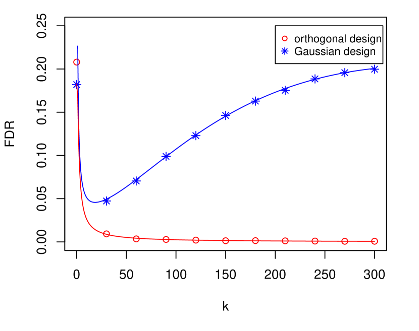
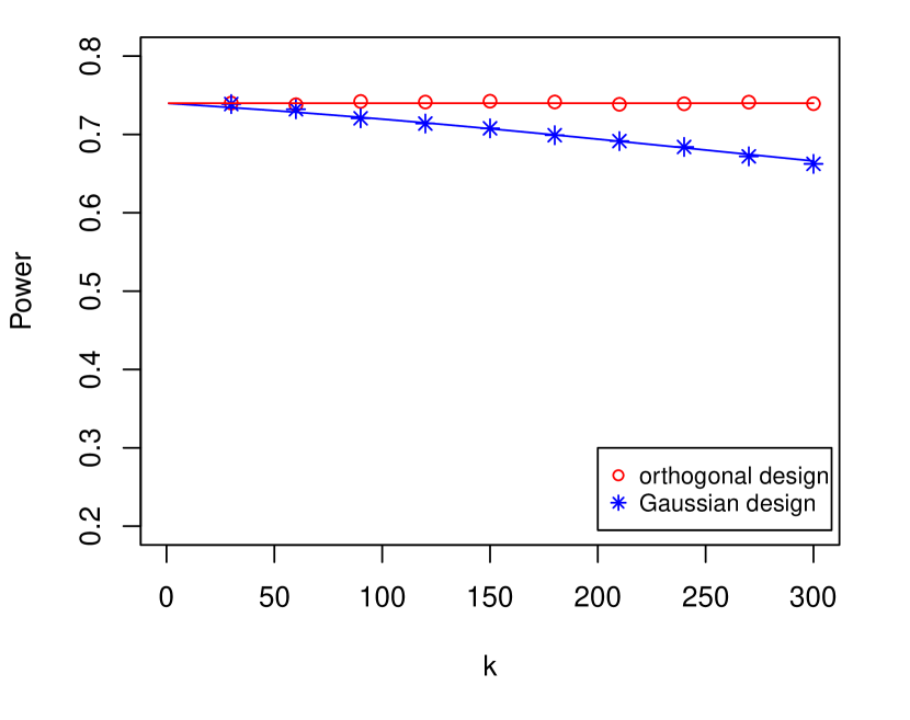
Figure 1: Estimated and predicted FDR and power of the lasso with $\lambda=3.717$ as a function of $k=\|\beta\|_{\ell_{0}}$. The entries of the Gaussian design are i.i.d. $\mathcal{N}(0,1/n)$. In both graphs, $n=p=1000$ and $\beta_{1},\ldots,\beta_{k}$ are independent normal random variables with mean $0$ and standard deviation equal to $3\lambda$. Each data point is a value estimated from 500 replicated experiments. Solid lines represent predicted curves. The predictions for the Gaussian design are based on the extension of the results in [6], see Appendix B.

Section 4 develops heuristic arguments to conclude on a perhaps surprising and disappointing note: if the columns of the design matrix are realizations of independent random variables, then independently on how large we select $\lambda$ nonadaptively, one can never be sure that the FDR of the lasso solution is controlled below some $q^{\star}=q^{\star}(n/p)>0$. The inability to control the FDR at a prescribed level is intimately connected to the shrinkage of the regression estimates, see Section 4.2.

Under a Gaussian design, we can in fact predict the asymptotic FDR of the lasso in the high signal-to-noise regime in which the magnitudes of the nonzero regression coefficients lie far above $\lambda$. Letting $\text{FDR}_{\text{lasso}}(\beta,\lambda)$ be the FDR of the lasso by employing $\lambda$ as a regularization parameter, a heuristic inspired by results in [6] gives

$$\lim_{p,n\rightarrow\infty}\,\,\inf_{\lambda}\,\,\sup_{\beta:\|\beta\|_{\ell_{0}}\leq k}\text{FDR}_{\text{lasso}}(\beta,\lambda)\geq q^{\star}(\epsilon,\delta),$$ (1.18)

where in the limit, $n/p\rightarrow\delta>0$ and $k/p\rightarrow\epsilon>0$. In Appendix B, we give explicit formulas for the lower limit $q^{\star}(\epsilon,\delta)$. Before continuing, we emphasize that we do not prove (1.18) rigorously, and only provide a heuristic justification. Now the accuracy of the prediction $q^{\star}$ is illustrated in Figure 2, where it is compared with FDR estimates from a simulation study with a Gaussian design as before, and a value of the nonzero coefficients set to $1,000\lambda$ and $\lambda=300$. The figure shows excellent agreement between predicted and observed behaviors. According to Figure 2, when $n/p=2,1$, or $0.5$, then independently on how large $\lambda$ is used one cannot be sure that the FDR is controlled below the values $0.08,0.27$, or $0.6$, respectively. We also note a singularity in the predicted curve for $n/p=1/2$, which occurs exactly at the point of the classical phase-transition curve in compressive sensing (or weak-threshold) of [22]. All of this is explained in Appendix B.

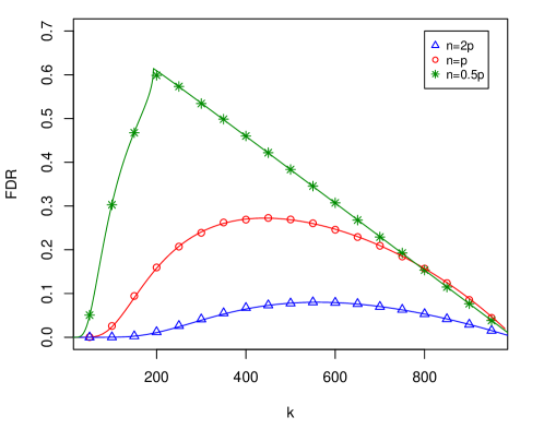
Figure 2: Simulated (markers) and predicted (lines) FDR in the high signal-to-noise regime as a function of the number of nonzero regression coefficients. Here, the design is $n\times p$ Gaussian with $p=1,000$. The formulas for the predicted curves are in Appendix B.

1.7 Contributions and outline

This paper introduces a novel method for sparse regression and variable selection, which is inspired by powerful adaptive ideas in multiple testing. We conclude this introduction by summarizing our contributions as well as outlining the rest of the paper. In Section 2, we demonstrate an efficient algorithm for computing the SLOPE solution. This algorithm is based on a linear time algorithm for computing the prox to the sorted $\ell_{1}$ norm (after sorting), and is new. In Section 3, we prove that SLOPE with the sequence $\lambda_{\text{BH}}$ controls the FDR under orthogonal designs. In Section 4, we detail the inherent limitations on the FDR level and the power which can be obtained with model selection methods based on $\ell_{1}$-like penalties. In this section, we also derive the predictions introduced in Section 1.6. A positive consequence of our understanding of FDR control is that it leads to an adjusted sequence $\{\lambda_{i}\}$ of parameters for use in SLOPE; see Section 4.3. Furthermore, in Section 5, we report on empirical findings demonstrating the following properties:

• First, when the number of non-nulls (the number of nonzero coefficients in the regression model) is not too large, SLOPE controls the FDR at a reasonable level, see Section 5.1. This holds provided that the columns of the design matrix are not strongly correlated. At the same time, the method has more power in detecting true regressors than the lasso and other competing methods. Therefore, just as the BH procedure, SLOPE controls a Type I error while enjoying greater power—albeit in a restricted setting.

• Second, in Section 5.2, we change our point of view and regard SLOPE purely as an estimation procedure. There we use SLOPE to select a subset of variables, and then obtain coefficient estimates by regressing the response on this subset. We demonstrate that with the adjusted weights from Section 4.3, this two-step procedure has good estimation properties even in situations when the input is not sparse at all. These good properties come from FDR control together with power in detecting nonzero coefficients. Indeed, a procedure selecting too many irrelevant variables would result in a large variance and distort the coefficient estimates of those variables in the model. At the same time, we need power as we would otherwise suffer from a large bias. Finally in Section 5.2, we shall see that the performance of SLOPE is not very sensitive to the choice of the parameter $q$ specifying the nominal FDR level.

Section 6 concludes the paper with a short discussion and questions we leave open for future research.

Finally, it goes without saying that our methods apply to multiple testing with correlated test statistics. Assume that $n\leq p$. Then multiplying the equation $y=X\beta+z$ on both sides by the pseudo inverse $X^{\dagger}$ of $X$ yields

$$y^{\prime}=(X^{\dagger})^{\prime}y\sim\mathcal{N}(\beta,\Sigma),$$

where $\Sigma=(X^{\prime}X)^{-1}$ whenever $X$ has full column rank. Hence, procedures for controlling the FDR in the linear model translate into procedures for testing the means of a multivariate Gaussian distribution. Our simulations in Section 5.1 illustrate that under sparse scenarios SLOPE has better properties than the BH procedure applied to marginal test statistics—with or without adjustment for correlation—in this context.

As a last remark, SLOPE is looking for a trade-off between the residual sum of squares and the sorted $\ell_{1}$ norm but we could equally contemplate using the sorted $\ell_{1}$ norm in other penalized estimation problems. Consider the Dantzig selector [17] which, assuming that the columns of $X$ are normalized, takes the form

$$\min_{b\in\mathbb{R}^{p}}\,\|b\|_{\ell_{1}}\quad\text{s.~{}t.}\quad\|X^{\prime}(y-Xb)\|_{\ell_{\infty}}\leq\lambda.$$ (1.19)

One can naturally use the ideas presented in this paper to tighten this in several ways, and one proposal is this: take a sequence $\lambda_{1}\geq\lambda_{2}\geq\ldots\geq\lambda_{p}\geq 0$ and consider

$$\min_{b\in\mathbb{R}^{p}}\,\|b\|_{\ell_{1}}\quad\text{s.~{}t.}\quad X^{\prime}(y-Xb)\in C_{\lambda},$$ (1.20)

where $C_{\lambda}$ is as in Proposition 1.1, see (1.9). With $\lambda_{1}=\lambda$, the constraint on the residual vector in (1.20) is tighter than that in (1.19). Indeed, setting $w=X^{\prime}(y-Xb)$, the feasible set in (1.19) is of the form $|w|_{(1)}\leq\lambda_{1}$ while that in the sorted version is $|w|_{(1)}\leq\lambda_{1}$, $|w|_{(1)}+|w|_{(2)}\leq\lambda_{1}+\lambda_{2}$, $|w|_{(1)}+|w|_{(2)}+|w|_{(3)}\leq\lambda_{1}+\lambda_{2}+\lambda_{3}$ and so on. Hence, the sorted version appears to shrink less and is more liberal.

2 Algorithms

In this section, we present effective algorithms for computing the solution to SLOPE (1.10), which rely on the numerical evaluation of the proximity operator (prox) to the sorted $\ell_{1}$ norm. Hence, we first develop a fast algorithm for computing the prox.

2.1 Preliminaries

Given $y\in\mathbb{R}^{n}$ and $\lambda_{1}\geq\lambda_{2}\geq\cdots\geq\lambda_{n}\geq 0$, the prox to the sorted $\ell_{1}$ norm is the unique solution to

$$\operatorname{prox}_{\lambda}(y)=\operatorname{argmin}_{x\in\mathbb{R}^{n}}\,\,{\textstyle\frac{1}{2}}\|y-x\|_{\ell_{2}}^{2}+\sum_{i=1}^{n}\lambda_{i}|x|_{(i)}.$$ (2.1)

Without loss of generality we can make the following assumption:

Assumption 2.1.

The vector $y$ obeys $y_{1}\geq y_{2}\geq\cdots\geq y_{n}\geq 0$.

At the solution to (2.1), the sign of each $x_{i}\neq 0$ will match that of $y_{i}$. It therefore suffices to solve the problem for $|y|$ and restore the signs in a post-processing step, if needed. Likewise, note that applying any permutation $P$ to $y$ results in a solution $Px$. We can thus choose a permutation that sorts the entries in $y$ and apply its inverse to obtain the desired solution.

Proposition 2.2.

Under Assumption 2.1, the solution $x$ to (2.1) satisfies $x_{1}\geq x_{2}\geq\cdots\geq x_{n}\geq 0$.

Proof Suppose that $x_{i}<x_{j}$ for $i<j$ (and $y_{i}>y_{j}$), and form a copy $x^{\prime}$ of $x$ with entries $i$ and $j$ exchanged. Letting $f$ be the objective functional in (2.1), we have

$$f(x)-f(x^{\prime})={\textstyle\frac{1}{2}}(y_{i}-x_{i})^{2}+{\textstyle\frac{1}{2}}(y_{j}-x_{j})^{2}-{\textstyle\frac{1}{2}}(y_{i}-x_{j})^{2}-{\textstyle\frac{1}{2}}(y_{j}-x_{i})^{2}.$$

This follows from the fact that the sorted $\ell_{1}$ norm takes on the same value at $x$ and $x^{\prime}$ and that all the quadratic terms cancel but those for $i$ and $j$. This gives

$$f(x)-f(x^{\prime})=x_{j}y_{i}-x_{i}y_{i}+x_{i}y_{j}-x_{j}y_{j}=(x_{j}-x_{i})(y_{i}-y_{j})>0,$$

which shows that the objective $x^{\prime}$ is strictly smaller, thereby contradicting optimality of $x$.  

Under Assumption 2.1 we can reformulate (2.1) as

$$\begin{array}[]{ll}\text{minimize}&\quad{\textstyle\frac{1}{2}}\|y-x\|_{\ell_{2}}^{2}+\sum_{i=1}^{n}\lambda_{i}x_{i}\\ \text{subject to}&\quad x_{1}\geq x_{2}\geq\cdots\geq x_{n}\geq 0.\end{array}$$ (2.2)

In other words, the prox is the solution to a quadratic program (QP). However, we do not suggest performing the prox calculation by calling a standard QP solver, rather we introduce a dedicated $O(n)$ algorithm we present next. For further reference, we record the Karush-Kuhn-Tucker (KKT) optimality conditions for this QP.

Primal feasibility: $x_{1}\geq x_{2}\geq\cdots\geq x_{n}\geq 0$.

Dual feasibility: $\mu\in\mathbb{R}^{n}$ obeys $\mu\geq 0$.

Complementary slackness: $\mu_{i}(x_{i}-x_{i+1})=0$ for all $i=1,\ldots,n$ (with the convention that $x_{n+1}=0$).

Stationarity of the Lagrangian:

$$x_{i}-y_{i}+\lambda_{i}-(\mu_{i}-\mu_{i-1})=0$$

with the convention that $\mu_{0}=0$).

2.2 A fast prox algorithm

Lemma 2.3.

Suppose $(y-\lambda)_{+}$ is nonincreasing, then the solution to (2.1) obeys

$$\operatorname{prox}_{\lambda}(y)=(y-\lambda)_{+}.$$

Proof Set $x=(y-\lambda)_{+}$, which by assumption is primal feasible, and let $i_{0}$ be the last index such that $y_{i}-\lambda_{i}>0$. Set $\mu_{1}=\mu_{2}=\ldots=\mu_{i_{0}}=0$ and for $j>i_{0}$, recursively define

$$\mu_{j}=\mu_{j-1}-(y_{j}-\lambda_{j})\geq 0.$$

Then it is straightforward to check that the pair $(x,\mu)$ obeys the KKT optimality conditions from Section 2.1  

We now introduce the FastProxSL1 algorithm (Algorithm 1) for computing the prox: for pedagogical reasons we introduce it in its simplest form before presenting in Section 2.3 a stack implementation running in $O(n)$ flops.

Algorithm 1 FastProxSL1

  input: Nonnegative and nonincreasing sequences $y$ and $\lambda$.

  while $y-\lambda$ is not nonincreasing do

     Identify strictly increasing subsequences, i.e. segments $i:j$ such that

$$y_{i}-\lambda_{i}<y_{i+1}-\lambda_{i+1}<\ldots<y_{j}-\lambda_{j}.$$ (2.3)

     Replace the values of $y$ over such segments by their average value: for $k\in\{i,i+1,\ldots,j\}$

$$y_{k}\leftarrow\frac{1}{j-i+1}\sum_{i\leq k\leq j}y_{k}.$$

     Replace the values of $\lambda$ over such segments by their average value: for $k\in\{i,i+1,\ldots,j\}$

$$\lambda_{k}\leftarrow\frac{1}{j-i+1}\sum_{i\leq k\leq j}\lambda_{k}.$$

  end while

  output: $x=(y-\lambda)_{+}$.

This algorithm, which obviously terminates in at most $n$ steps, is simple to understand: we simply keep on averaging until the monotonicity property holds, at which point the solution is known in closed form thanks to Lemma 2.3. The key point establishing the correctness of the algorithm is that the update does not change the value of the prox. This is formalized below.

Lemma 2.4.

Let $(y^{+},\lambda^{+})$ be the updated value of $(y,\lambda)$ after one pass in Algorithm 1. Then

$$\operatorname{prox}_{\lambda}(y)=\operatorname{prox}_{\lambda^{+}}(y^{+}).$$

Proof We first claim that the prox has to be constant over any monotone segment of the form

$$y_{i}-\lambda_{i}\leq y_{i+1}-\lambda_{i+1}\leq\ldots\leq y_{j}-\lambda_{j}.$$

To see why this is true, set $x=\operatorname{prox}_{\lambda}(y)$ and suppose the contrary: then over a segment as above, there is $k\in\{i,i+1,\ldots,j-1\}$ such that $x_{k}>x_{k+1}$ (we cannot have a strict inequality in the other direction since $x$ has to be primal feasible). By complementary slackness, $\mu_{k}=0$. This gives

$$x_{k} =y_{k}-\lambda_{k}-\mu_{k-1}$$

$$x_{k+1} =y_{k+1}-\lambda_{k+1}+\mu_{k+1}.$$

Since $y_{k+1}-\lambda_{k+1}\geq y_{k}-\lambda_{k}$ and $\mu\geq 0$, we have $x_{k}\leq x_{k+1}$, which is a contradiction.

Now an update replaces an increasing segment as in (2.3) with a constant segment and we have just seen that both proxes must be constant over such segments. Now consider the cost function associated with the prox with parameter $\lambda$ and input $y$ over an increasing segment as in (2.3),

$$\sum_{i\leq k\leq j}\Bigl{\{}{\textstyle\frac{1}{2}}(y_{k}-x_{k})^{2}+\lambda_{k}x_{k}\Bigr{\}}.$$ (2.4)

Since all the variables $x_{k}$ must be equal to some value $z$ over this block, this cost is equal to

$$\sum_{i\leq k\leq j}\Bigl{\{}{\textstyle\frac{1}{2}}(y_{k}-z)^{2}+\lambda_{k}z\Bigr{\}} =\sum_{k}{\textstyle\frac{1}{2}}(y_{k}-\bar{y})^{2}+\sum_{i\leq k\leq j}\Bigl{\{}{\textstyle\frac{1}{2}}(\bar{y}-z)^{2}+\bar{\lambda}z\Bigr{\}}$$

$$=\sum_{k}{\textstyle\frac{1}{2}}(y_{k}-\bar{y})^{2}+\sum_{i\leq k\leq j}\Bigl{\{}{\textstyle\frac{1}{2}}(y_{k}^{+}-z)^{2}+\bar{\lambda}_{k}^{+}z\Bigr{\}},$$

where $\bar{y}$ and $\bar{\lambda}$ are block averages. The second term in the right-hand side is the cost function associated with the prox with parameter $\lambda^{+}$ and input $y^{+}$ over the same segment since all the variables over this segment must also take on the same value. Therefore, it follows that replacing each appearance of block sums as in (2.4) in the cost function yields the same minimizer. This proves the claim.  

In summary, the FastProxSL1 algorithm finds the solution to (2.1) in a finite number of steps.

2.3 Stack-based algorithm for FastProxSL1

As stated earlier, it is possible to obtain an $O(n)$ implementation of FastProxSL1. Below we present a stack-based approach. We use tuple notation $(a,b)_{i}=(c,d)$ to denote $a_{i}=c$, $b_{i}=d$.

Algorithm 2 Stack-based algorithm for FastProxSL1.

1:  input: Nonnegative and nonincreasing sequences $y$ and $\lambda$.

2:  # Find optimal group levels

3:  $t\leftarrow 0$

4:  for $k=1$ to $n$ do

5:     $t\leftarrow t+1$

6:     $(i,j,s,w)_{t}=(k,\ k,\ y_{i}-\lambda_{i},\ (y_{i}-\lambda_{i})_{+})$

7:     while $(t>1)$ and $(w_{t-1}\leq w_{t})$ do

8:        $(i,j,s,w)_{t-1}\leftarrow(i_{t-1},\ j_{t},\ s_{t-1}+s_{t},(\frac{j_{t-1}-i_{t-1}+1}{j_{t}-i_{t-1}+1}\cdot s_{t-1}+\frac{j_{t}-i_{t}+1}{j_{t}-i_{i-1}+1}\cdot s_{t})_{+}$)

9:        Delete $(i,j,s,w)_{t}$, $t\leftarrow t-1$

10:     end while

11:  end for

12:  # Set entries in $x$ for each block

13:  for $\ell=1$ to $t$ do

14:     for $k=i_{\ell}$ to $j_{\ell}$ do

15:        $x_{k}\leftarrow w_{\ell}$

16:     end for

17:  end for

For the complexity of the algorithm note that we create a total of $n$ new tuples. Each of these tuple is merged into a previous tuple at most once. Since the merge takes a constant amount of time the algorithm has the desired ${O}(n)$ complexity.

With this paper, we are making available a C, a Matlab, and an R implementation of the stack-based algorithm at http://www-stat.stanford.edu/~candes/SortedL1. The algorithm is also included in the current version of the TFOCS package available here http://cvxr.com, see [8]. To give an idea of the speed, we applied the code to a series of vectors with fixed length and varying sparsity levels. The average runtimes measured on a MacBook Pro equipped with a 2.66 GHz Intel Core i7 are reported in Table 1.

	$p=10^{5}$	$p=10^{6}$	$p=10^{7}$
Total prox time (sec.)	9.82e-03	1.11e-01	1.20e+00
Prox time after normalization (sec.)	6.57e-05	4.96e-05	5.21e-05

Table 1: Average runtimes of the stack-based prox implementation with normalization steps (sorting and sign changes) included, respectively excluded.

2.4 Proximal algorithms for SLOPE

With a rapidly computable algorithm for evaluating the prox, efficient methods for computing the SLOPE solution (1.10) are now a stone’s throw away. Indeed, we can entertain a proximal gradient method which goes as in Algorithm 3.

Algorithm 3 Proximal gradient algorithm for SLOPE (1.10)

0:  $b^{0}\in\mathbb{R}^{p}$

1:  for $k=0,1,\ldots$ do

2:     $b^{k+1}=\operatorname{prox}_{\lambda}(b^{k}-t_{k}X^{\prime}(Xb^{k}-y))$

3:  end for

It is well known that the algorithm converges (in the sense that $f(b^{k})$, where $f$ is the objective functional, converges to the optimal value) under some conditions on the sequence of step sizes $\{t_{k}\}$. Valid choices include step sizes obeying $t_{k}<2/\|X\|^{2}$ and step sizes obtained by backtracking line search, see [8, 7].

Many variants are of course possible and one may entertain accelerated proximal gradient methods in the spirit of FISTA, see [7] and [29, 30]. The scheme below is adapted from [7].

Algorithm 4 Accelerated proximal gradient algorithm for SLOPE (1.10)

0:  $b^{0}\in\mathbb{R}^{p}$, and set $a^{0}=b^{0}$ and $\theta_{0}=1$

1:  for $k=0,1,\ldots$ do

2:     $b^{k+1}=\operatorname{prox}_{\lambda}(a^{k}-t_{k}X^{\prime}(Xa^{k}-y))$

3:     $\theta_{k+1}^{-1}=\frac{1}{2}(1+\sqrt{1+4/\theta_{k}^{2}})$

4:     $a^{k+1}=b^{k+1}+\theta_{k+1}(\theta_{k}^{-1}-1)(b^{k+1}-b^{k})$

5:  end for

The code used for the numerical experiments uses a straightforward implementation of the standard FISTA algorithm, along with problem-specific stopping criteria. Standalone Matlab and R implementations of the algorithm are available at the website listed in Section 2.3. TFOCS implements Algorithms 3 and 4 as well as many variants; for instance, the Matlab code below prepares the prox and then solves the SLOPE problem,

prox = prox_Sl1(lambda);
beta = tfocs( smooth_quad, { X, -y }, prox, beta0, opts );

Here beta0 is an initial guess (which can be omitted) and opts are options specifying the methods and parameters one would want to use, please see [8] for details. There is also a one-liner with default options which goes like this:

beta  = solver_SLOPE( X, y, lambda);

2.5 Duality-based stopping criteria

To derive the dual of (1.10) we first rewrite it as

$$\mathop{\hbox{minimize}}_{b,r}\quad{\textstyle\frac{1}{2}}r^{\prime}r+J_{\lambda}(b)\quad\mathop{\hbox{subject to}}\quad Xb+r=y.$$

The dual is then given by

$$\mathop{\hbox{maximize}}_{w}\quad\mathcal{L}(b,r,w),$$

where

$$\mathcal{L}(b,r,w) := \inf_{b,r}\ \{{\textstyle\frac{1}{2}}r^{\prime}r+J_{\lambda}(b)-w^{\prime}(Xb+r-y)\}$$

$$= w^{\prime}y-\sup_{r}\ \{w^{\prime}r-{\textstyle\frac{1}{2}}r^{\prime}r\}-\sup_{b}\ \{(X^{\prime}w)^{\prime}b-J_{\lambda}(b)\}.$$

The first supremum term evaluates to ${\textstyle\frac{1}{2}}w^{\prime}w$ by choosing $r=w$. The second term is the conjugate function $J^{*}$ of $J$ evaluated at $v=X^{\prime}w$, which can be shown to reduce to

$$J^{*}_{\lambda}(v):=\sup_{b}\ \{v^{\prime}b-J_{\lambda}(b)\}=\begin{cases}0&v\in C_{\lambda},\\ +\infty&\mbox{otherwise},\end{cases}$$

where the set $C_{\lambda}$ is given by (1.9). The dual problem is thus given by

$$\mathop{\hbox{maximize}}_{w}\quad w^{\prime}y-{\textstyle\frac{1}{2}}w^{\prime}w\quad\mathop{\hbox{subject to}}\quad w\in C_{\lambda}.$$

The dual formulation can be used to derive appropriate stopping criteria. At the solution we have $w=r$, which motivates estimating a dual point by setting $\hat{w}=r=:y-Xb$. At this point the primal-dual gap at $b$ is the difference between the primal and dual objective:

$$\delta(b)=(Xb)^{\prime}(Xb-y)+J_{\lambda}(b).$$

However, $\hat{w}$ is not guaranteed to be feasible, i.e., we may not have $\hat{w}\in C_{\lambda}$. Therefore we also need to compute a level of infeasibility of $\hat{w}$, for example

$$\mbox{infeasi}(\hat{w})=\max\Big{\{}0,\ \max_{i}\sum_{j\leq i}(|\hat{w}|_{(j)}-\lambda_{j})\Big{\}}.$$

The algorithm used in the numerical experiments terminates whenever both the infeasibility and primal-dual gap are sufficiently small. In addition, it imposes a limit on the total number of iterations to ensure termination.

3 FDR Control Under Orthogonal Designs

In this section, we prove FDR control in the orthogonal design, namely, Theorem 1.3. As we have seen in Section 1, the SLOPE solution reduces to

$$\min_{b\in\mathbb{R}^{p}}\,{\textstyle\frac{1}{2}}\|\tilde{y}-b\|_{\ell_{2}}^{2}+\sum_{i=1}^{p}\lambda_{i}|b|_{(i)},$$

where $\tilde{y}=X^{\prime}y\sim\mathcal{N}(\beta,I_{p})$. From this, it is clear that it suffices to consider the setting in which $y\sim\mathcal{N}(\beta,I_{n})$, which we assume from now on.

We are thus testing the $n$ hypotheses $H_{i}:\beta_{i}=0$, $i=1,\ldots,n$ and set things up so that the first $n_{0}$ hypotheses are null, i.e. $\beta_{i}=0$ for $i\leq n_{0}$. The SLOPE solution is

$$\hat{\beta}=\text{arg min}\,{\textstyle\frac{1}{2}}\|y-b\|_{\ell_{2}}^{2}+\sum_{i=1}^{n}\lambda_{i}|b|_{(i)}$$ (3.1)

with $\lambda_{i}=\Phi^{-1}(1-iq/2n)$. We reject $H_{i}$ if and only if $\hat{\beta}_{i}\neq 0$. Letting $V$ (resp. $R$) be the number of false rejections (resp. the number of rejections) or, equivalently, the number of indices in $\{1,\ldots,n_{0}\}$ (resp. in $\{1,\ldots,n\}$) for which $\hat{\beta}_{i}\neq 0$, we have

$$\text{FDR}=\operatorname{\mathbb{E}}\left[\frac{V}{R\vee 1}\right]=\sum_{r=1}^{n}\operatorname{\mathbb{E}}\left[\frac{V}{r}\mathbbm{1}_{\left\{{R=r}\right\}}\right]=\sum_{r=1}^{n}\frac{1}{r}\operatorname{\mathbb{E}}\left[\sum_{i=1}^{n_{0}}\mathbbm{1}_{\left\{{H_{i}\text{ is rejected}}\right\}}\mathbbm{1}_{\left\{{R=r}\right\}}\right].$$ (3.2)

The proof of Theorem 1.3 now follows from the two key lemmas below.

Lemma 3.1.

Let $H_{i}$ be a null hypothesis and let $r\geq 1$. Then

$$\{\text{\rm$y$: $H_{i}$ is rejected and $R=r$}\}=\{\text{\rm$y$: $|y_{i}|>\lambda_{r}$ and $R=r$}\}.$$

Lemma 3.2.

Consider applying the SLOPE procedure to $\tilde{y}=(y_{1},\ldots,y_{i-1},y_{i+1},\ldots,y_{n})$ with weights $\tilde{\lambda}=(\lambda_{2},\ldots,\lambda_{n})$ and let $\tilde{R}$ be the number of rejections this procedure makes. Then with $r\geq 1$,

$$\{\text{\rm$y$: $|y_{i}|>\lambda_{r}$ and $R=r$}\}\subset\{y:\text{\rm$|y_{i}|>\lambda_{r}$ and $\tilde{R}=r-1$}\}.$$

To see why these intermediate results give Theorem 1.3, observe that

$$\operatorname{\mathbb{P}}(\text{$H_{i}$ rejected and $R=r$}) \leq\operatorname{\mathbb{P}}(\text{$|y_{i}|\geq\lambda_{r}$ and $\tilde{R}=r-1$})$$

$$=\operatorname{\mathbb{P}}(|y_{i}|\geq\lambda_{r})\operatorname{\mathbb{P}}(\tilde{R}=r-1)$$

$$=\frac{qr}{n}\operatorname{\mathbb{P}}(\tilde{R}=r-1),$$

where the inequality is a consequence of the lemmas above and the first equality follows from the independence between $y_{i}$ and $\tilde{y}$. Plugging this inequality into (3.2) gives

$$\text{FDR}=\sum_{r=1}^{n}\frac{1}{r}\sum_{i=1}^{n_{0}}\operatorname{\mathbb{P}}(\text{$H_{i}$ rejected and $R=r$})\leq\sum_{r\geq 1}\frac{qn_{0}}{n}\operatorname{\mathbb{P}}(\tilde{R}=r-1)=\frac{qn_{0}}{n},$$

which finishes the proof.

3.1 Proof of Lemma 3.1

We begin with a lemma we shall use more than once.

Lemma 3.3.

Consider a pair of nonincreasing and nonnegative sequences $y_{1}\geq y_{2}\geq\ldots\geq y_{n}\geq 0$, $\lambda_{1}\geq\lambda_{2}\geq\ldots\geq\lambda_{n}\geq 0$, and let $\hat{b}$ be the solution to

$$\begin{array}[]{ll}\text{\rm minimize}&\quad f(b)=\,{\textstyle\frac{1}{2}}\|y-b\|_{\ell_{2}}^{2}+\sum_{i=1}^{n}\lambda_{i}b_{i}\\ \text{\rm subject to}&\quad b_{1}\geq b_{2}\geq\ldots\geq b_{n}\geq 0.\end{array}$$

If $\hat{b}_{r}>0$ and $\hat{b}_{r+1}=0$, then for every $j\leq r$, it holds that

$$\sum_{i=j}^{r}(y_{i}-\lambda_{i})>0$$ (3.3)

and for every $j\geq r+1$,

$$\sum_{i=r+1}^{j}(y_{i}-\lambda_{i})\leq 0.$$ (3.4)

Proof To prove (3.3), consider a new feasible sequence $b$, which differs from $\hat{b}$ only by subtracting a small positive scalar $h<\hat{b}_{r}$ from $\hat{b}_{j},\ldots,\hat{b}_{r}$. Now

$$f(b)-f(\hat{b})=h\sum_{i=j}^{r}(y_{i}-\lambda_{i}-\hat{b}_{i})+h^{2}\sum_{i=j}^{r}{\textstyle\frac{1}{2}}.$$

Taking the limit as $h$ goes to zero, the optimality of $\hat{b}$ implies that $\sum_{i=j}^{r}(y_{i}-\lambda_{i}-\hat{b}_{i})\geq 0$, which gives

$$\sum_{i=j}^{r}(y_{i}-\lambda_{i})\geq\sum_{i=j}^{r}\hat{b}_{i}>0.$$

For the second claim (3.4), consider a new sequence $b$, which differs from $\hat{b}$ by replacing $\hat{b}_{r+1},\ldots,\hat{b}_{j}$ with a positive scalar $0<h<\hat{b}_{r}$. Now observe that

$$f(b)-f(\hat{b})=-h\sum_{i=r+1}^{j}(y_{i}-\lambda_{i})+h^{2}\sum_{i=r+1}^{j}{\textstyle\frac{1}{2}}.$$

The claim follows from the optimality of $\hat{b}$.  

It is now straightforward so see how these simple relationships give Lemma 3.1. Observe that when $R=r$, we must have $|y|_{(r)}>\lambda_{r}$ and $|y|_{(r+1)}\leq\lambda_{r+1}$. Hence, if $H_{1}$ is rejected, it must hold that $|y_{1}|\geq|y|_{(r)}>\lambda_{r}$. This shows that $\{\text{$H_{1}$ is rejected and $R=r$}\}\subset\{\text{$|y_{1}|>\lambda_{r}$ and $R=r$}\}$. Conversely, assume that $|y_{1}|>\lambda_{r}$ and $R=r$. Then $H_{1}$ must be rejected since $|y_{1}|>|y|_{(r+1)}$. This shows that $\{\text{$H_{1}$ is rejected and $R=r$}\}\supset\{\text{$|y_{1}|>\lambda_{r}$ and $R=r$}\}$.

3.2 Proof of Lemma 3.2

We assume without loss of generality that $y\geq 0$ (the extension to arbitrary signs is trivial). By assumption the solution to (3.1) with $\lambda_{i}=\Phi^{-1}(1-iq/2n)$ has exactly $r$ strictly positive entries, and we need to show that when $y_{1}$ is rejected, the solution to

$$\text{min}\,J(\tilde{b}):=\sum_{i=1}^{n-1}{\textstyle\frac{1}{2}}(\tilde{y}_{i}-\tilde{b}_{i})^{2}+\sum_{i=1}^{n-1}\tilde{\lambda}_{i}|\tilde{b}|_{(i)}$$ (3.5)

in which $\tilde{\lambda}_{i}=\lambda_{i+1}$ has exactly $r-1$ nonzero entries. We prove this in two steps:

• The optimal solution $\hat{b}$ to (3.5) has at least $r-1$ nonzero entries.

• The optimal solution $\hat{b}$ to (3.5) has at most $r-1$ nonzero entries.

3.2.1 Proof of (i)

Suppose by contradiction that $\hat{b}$ has fewer than $r-1$ entries; i.e., $\hat{b}$ has $j-1$ nonzero entries with $j<r$. Letting $I$ be those indices for which the rank of $\tilde{y}_{i}$ is between $j$ and $r-1$, consider a feasible point $b$ as in the proof of Lemma 3.3 defined as

$$b_{i}=\begin{cases}h&i\in I,\\ \hat{b}_{i}&\text{otherwise};\end{cases}$$

here, the positive scalar $h$ obeys $0<h<b_{(j-1)}$. By definition,

$$J(b)-J(\hat{b})=-h\sum_{i=j}^{r-1}(\tilde{y}_{(i)}-\tilde{\lambda}_{i})+h^{2}\sum_{i=j}^{r-1}{\textstyle\frac{1}{2}}.$$

Now

$$\sum_{j\leq i\leq r-1}\tilde{y}_{(i)}-\tilde{\lambda}_{i}=\sum_{j+1\leq i\leq r}\tilde{y}_{(i-1)}-\lambda_{i}\geq\sum_{j+1\leq i\leq r}y_{(i)}-\lambda_{i}>0.$$

The first equality follows from $\tilde{\lambda}_{i}=\lambda_{i+1}$, the first inequality from $y_{(i)}\leq\tilde{y}_{(i-1)}$ and the last from (3.3). By selecting $h$ small enough, this gives $J(b)<J(\hat{b})$, which contradicts the optimality of $\hat{b}$.

3.2.2 Proof of (ii)

The proof is similar to that of (i). Suppose by contradiction that $\hat{b}$ has more than $r-1$ entries; i.e. $\hat{b}$ has $j$ nonzero entries with $j\geq r$. Letting $I$ be those indices for which the rank of $\tilde{y}_{i}$ is between $r$ and $j$, consider a feasible point $b$ as in the proof of Lemma 3.3 defined as

$$b_{i}=\begin{cases}b_{i}-h&i\in I\\ \hat{b}_{i}&\text{otherwise};\end{cases}$$

here, the positive scalar $h$ obeys $0<h<b_{(j)}$. By definition,

$$J(b)-J(\hat{b})=h\sum_{i=r}^{j}(\tilde{y}_{(i)}-\tilde{\lambda}_{i}-\hat{b}_{(i)})+h^{2}\sum_{i=r}^{j}{\textstyle\frac{1}{2}}.$$

Now

$$\sum_{r\leq i\leq j}(\tilde{y}_{(i)}-\tilde{\lambda}_{i})=\sum_{r+1\leq i\leq j+1}(y_{(i)}-\lambda_{i})\leq 0.$$

The equality follows from the definition and the inequality from (3.4). By selecting $h$ small enough, this gives $J(b)<J(\hat{b})$, which contradicts the optimality of $\hat{b}$.

4 FDR Control Under General Designs

4.1 The notion of FDR in the linear model

We consider the multiple testing problem in which we wish to decide whether each of the $p$ regression coefficients in the linear model (1.1) is zero or not. Now the notion of FDR control in this situation is delicate and it is best to present the precise context in which our results hold as to avoid any kind of misunderstanding. We work with a generative model

$$y=X\beta+z$$

for the data in which the errors are i.i.d. zero-mean Gaussian random variables. In other words, we assume that the (full) linear model is correct and wish to know which of the coefficients $\beta_{i}$ are nonzero. For example, in a medical imaging application, $\beta$ may be the concentrations of hydrogen at various locations in the body (different tissues are characterized by different concentration levels) and while we cannot observe such concentrations directly, they can be measured indirectly by magnetic resonance. In this case, the linear model above holds, the object of inference is a well-defined physical quantity, and it makes sense to test whether there are locations whose concentration exceeds a prescribed level. Another example may concern gene mapping studies in which we wish to identify which of the many genes are associated with a given phenotype. Here, there are mutations that affect the phenotype and others that do not so that—assuming the correctness of the linear model—there are true (and false) discoveries to be made. We are thus concerned with a true linear model in which the notion of a true regressor along with the value of its regression coefficient has a clear meaning, and can be explained in the language of the respective science. In contrast, we are not concerned with the use of the linear model as means of an interpretative model, which, while being inexact, may be used to summarize a phenomenon of interest or predict future outcomes since it may not allow true and false discoveries.

Furthermore, we also wish to stay away from designs where the columns of $X$ (the variables) are highly correlated as in this case, the stringent definition we adopt for FDR (expected proportion of incorrectly selected variables) may not be the right notion of Type I error, see the discussion in [33]. Hence, we shall present the performance of different selection methods on seemingly simple examples, where the columns of the design matrix are only slightly correlated or where they are generated as independent random variables. As we shall see, while small correlations can already lead to many variable selection problems, model selection procedures based on the sorted $\ell_{1}$ norm can work well under sparsity, i.e., when the number of true regressors is comparably small.

4.2 Loss of FDR control due to shrinkage

As briefly mentioned in the Introduction, methods using convex surrogates for sparsity, such as the $\ell_{1}$ or sorted $\ell_{1}$ norms, can have major difficulties in controlling the FDR. This phenomenon has to do with the shrinkage of regression coefficients, as we now explain.

We consider the lasso (1.5) for simplicity and assume that the columns of $X$ have unit norm. The optimality conditions for the lasso solution $\hat{\beta}$ take the form

$$\hat{\beta}=\eta_{\lambda}(\hat{\beta}-X^{\prime}(X\hat{\beta}-y)),$$ (4.1)

where $\eta_{\lambda}$ is the soft-thresholding operator, $\eta_{\lambda}(t)=\textrm{sgn}(t)(|t|-\lambda)_{+}$, applied componentwise; see [31, page 150]. Setting

$$v_{i}=\langle X_{i},\sum_{j\neq i}X_{j}(\beta_{j}-\hat{\beta}_{j})\rangle,$$ (4.2)

we can rewrite the optimality condition as

$$\hat{\beta}_{i}=\eta_{\lambda}(\beta_{i}+X_{i}^{\prime}z+v_{i}).$$ (4.3)

Observe that conditional on $X$, $X_{i}^{\prime}z\sim\mathcal{N}(0,1)$. In an orthogonal design, $v_{i}=0$ for all $i$, and taking $\lambda$ at the appropriate level (e.g., $\Phi^{-1}(1-q/2p)$) controls the FDR and even the FWER. Imagine now that $X$ has correlated columns and that $k$ regression coefficients are large. Then the lasso estimates of these coefficients will be shrunk towards zero by an amount roughly proportional to $\lambda$. The effect of this is that $v_{i}$ now looks like a noise term whose size is roughly proportional to $\lambda$ times the square root of $k$. In other words, there is an inflation of the ‘noise variance’ so that we should not be thresholding at $\lambda$ but at a higher value. The consequence is that the lasso procedure is too liberal and selects too many variables for which $\beta_{i}=0$; hence, the FDR becomes just too large. One can imagine using a higher value of $\lambda$. The problem, however, is that the if the coefficients are really large, the estimation bias is of size $\lambda$ so that the size of $v_{i}$ scales like $\lambda$ so there does not appear to be an easy way out (at least, as long as $\lambda$ is selected non-adaptively).

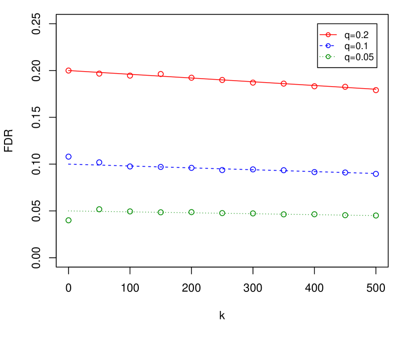
(a) Orthogonal design.

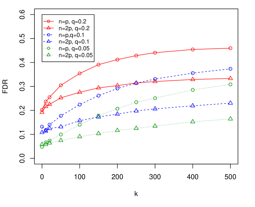
(b) Gaussian design.

Figure 3: Observed FDR of SLOPE with $\lambda=\lambda_{\text{BH}}$ for $p=5,000$. In (a), the straight lines indicate the nominal level of the BHq procedure, namely, $q(1-k/p)$.

Following this line of thought, one can make two qualitative predictions in the model with a few large regressors: (1) the problem tends to be more severe as the number of regressors increases, at least initially (when most of the variables are in the model, it gets harder to make false rejections), and (2) the problem tends to be more severe when the columns tend to be more correlated. Obviously, the problems with FDR control also apply to SLOPE. Figure 3 presents the estimated FDR of SLOPE both with an orthogonal design and a random Gaussian design in which $X$ has i.i.d. $\mathcal{N}(0,1/n)$ entries so that the columns nearly have unit norm. The sequence $\lambda$ is set to be $\lambda_{\text{BH}}$. In the first case, we work with $n=p=5,000$ and in the second with $n=p=5,000$ and $n=2p=10,000$. The value of the nonzero regression coefficients is set to $5\sqrt{2\log p}$. Figure 3(b) shows that SLOPE with a sequence of BH values no longer controls the FDR in the nonorthogonal case. In fact, the FDR increases with $k$ as predicted. The values of FDR are substantially smaller when $n=2p$ as compared to the case when $n=p$. This is naturally in line with our prediction since $\operatorname{\mathbb{E}}(X_{i}^{\prime}X_{j})^{2}=1/n$ for $i\neq j$ so that random vectors in dimension $n=5,000$ statistically exhibit higher sample correlations than vectors in a space of twice this size.

In closing, we have discussed the problem associated with the bias induced by large regression coefficients. Looking at (4.3), there are of course other sources of bias causing a variance inflation such as those coefficients $\beta_{j}\neq 0$ with vanishing estimates, i.e., $\hat{\beta}_{j}=0$.

4.3 Adjusting the regularizing sequence for SLOPE

Selecting a sequence $\{\lambda_{i}\}$ for use in SLOPE is an interesting research topic that is beyond the scope of this work. Having said this, an initial thought would be to work with the same sequence as in an orthogonal design, namely, with $\lambda_{i}=\lambda_{\text{BH}}(i)$ as in Theorem 1.3. However, we have demonstrated that this choice is too liberal and in this section, we use our qualitative insights to propose an intuitive adjustment. Our treatment here is informal.

Imagine we use $\lambda_{\text{BH}}$ and that there are $k$ large coefficients. To simplify notation, we suppose that $\beta_{1}\geq\beta_{2}\geq\ldots\beta_{k}\gg 1$ and let $\mathcal{S}$ be the support set $\{1,\ldots,k\}$. Assuming SLOPE correctly detects these variables and correctly estimates the signs of the regression coefficients, the estimate of the nonzero components is very roughly equal to

$$(X_{\mathcal{S}}^{\prime}X_{\mathcal{S}})^{-1}(X_{\mathcal{S}}^{\prime}y-\lambda_{\mathcal{S}}),$$

where $\lambda_{\mathcal{S}}=(\lambda_{\text{BH}}(1),\ldots,\lambda_{\text{BH}}(k))^{\prime}$ causing a bias approximately equal to

$$\operatorname{\mathbb{E}}X_{\mathcal{S}}(\beta_{\mathcal{S}}-\hat{\beta}_{\mathcal{S}})\approx X_{\mathcal{S}}(X_{\mathcal{S}}^{\prime}X_{\mathcal{S}})^{-1}\lambda_{\mathcal{S}}.$$

We now return to (4.3) and ask about the size of the variance inflation: in other words, what is the typical size of $X^{\prime}_{i}X_{\mathcal{S}}(X_{\mathcal{S}}^{\prime}X_{\mathcal{S}})^{-1}\lambda_{\mathcal{S}}$? For a Gaussian design where the entries of $X$ are i.i.d. $\mathcal{N}(0,1)$, it is not hard to see that for $i\notin\mathcal{S}$,

$$\operatorname{\mathbb{E}}(X^{\prime}_{i}X_{\mathcal{S}}(X_{\mathcal{S}}^{\prime}X_{\mathcal{S}})^{-1}\lambda_{\mathcal{S}})^{2}=\lambda_{\mathcal{S}}^{\prime}\operatorname{\mathbb{E}}(X_{\mathcal{S}}^{\prime}X_{\mathcal{S}})^{-1}\lambda_{\mathcal{S}}=\frac{\|\lambda_{\mathcal{S}}\|_{\ell_{2}}^{2}}{n-|\mathcal{S}|-1},$$

where the last equality uses the fact that the expected value of an inverse dimensional Wishart of dimension $k$ with $n$ degrees of freedom is equal to $I_{k}/(n-k-1)$.

This suggests a correction of the following form: we start with $\lambda_{1}=\lambda_{\text{BH}}(1)$. At the next stage, however, we need to account for the slight increase in variance so that we do not want to use $\lambda_{\text{BH}}(2)$ but rather

$$\lambda_{2}=\lambda_{\text{BH}}(2)\sqrt{1+\frac{\lambda_{1}^{2}}{n-2}}.$$

Continuing, this gives

$$\lambda_{i}=\lambda_{\text{BH}}(i)\sqrt{1+\frac{\sum_{j<i}\lambda_{j}^{2}}{n-i}}.$$ (4.4)

In our simulations, we shall use a variation on this idea and work with $\lambda_{1}=\lambda_{\text{BH}}(1)$ and for $i>1$,

$$\lambda_{i}=\lambda_{\text{BH}}(i)\sqrt{1+\frac{\sum_{j<i}\lambda_{\text{BH}}^{2}(j)}{n-i}}.$$ (4.5)

In practice, the performance of this slightly less conservative sequence does not differ from (4.4). Figure 4 plots the adjusted values given by (4.5). As is clear, these new values yield a procedure that is more conservative than that based on $\lambda_{\text{BH}}$.

(a) $q=0.2$.

(b) $q=0.05$.

Figure 4: Graphical representation of sequences $\{\lambda_{i}\}$ for $p=5000$. The solid line is $\lambda_{\text{BH}}$, the dashed (resp. dotted) line is $\lambda$ given by (4.5) for $n=p$ (resp. $n=2p$).

For small values of $q$, the sequence $\lambda_{i}$ is no longer decreasing. Rather it decreases until it reaches a minimum value and then increases. It would not make sense to use such a sequence—note that we would also lose convexity—and letting $k^{\star}=k(n,p,q)$ be the location of the global minimum, we shall work with

$$\lambda_{\text{BHc}}(i)=\begin{cases}\lambda_{i},&i\leq k^{\star},\\ \lambda_{k^{\star}},&i>k^{\star},\end{cases}\quad\text{with $\lambda_{i}$ as in \eqref{eq:LOL}}.$$ (4.6)

Working with $\lambda_{\text{BHc}}$, Figure 5 plots the observed FDR of SLOPE in the same setup as in Figure 3(b). For $n=p=5,000$, the values of the critical point $k^{\star}$ are $91$ for $q=0.05$, $141$ for $q=0.1$, and $279$ for $q=0.2$. For $n=2p=10,000$, they become $283$, $560$, and $2,\!976$, respectively. It can be observed that SLOPE keeps the FDR at a level close to the nominal level even after passing the critical point. When $n=p=5,000$ and $q=0.05$, which corresponds to the situation in which the critical point is earliest ($k^{\star}=91$), one can observe a slight increase in FDR above the nominal value when $k$ ranges from $100$ to $200$. It is also interesting to observe that FDR control is more difficult when the coefficients have moderate amplitudes rather than when they have large ones. Although this effect is very small, an interpretation is that the correction is not strong enough to account for the loss of power; that is, for not including a large fraction of true regressors.

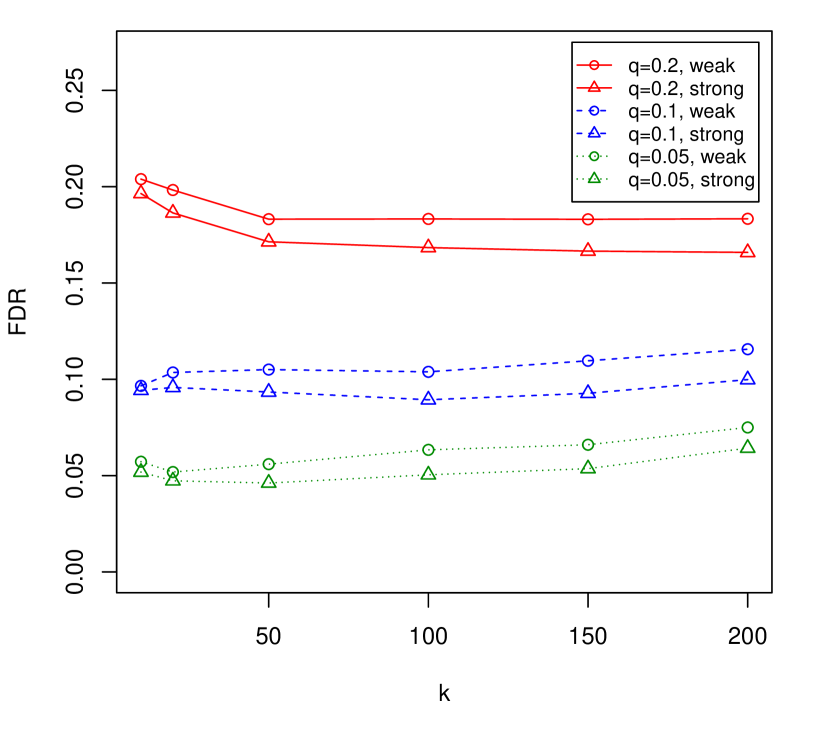
(a) $n=p=5,000$.

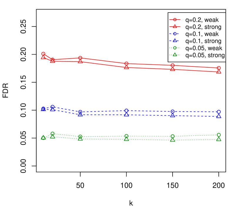
(b) $n=2p=10,000$.

Figure 5: FDR of SLOPE with $\lambda_{i}=\lambda_{\text{BHc}}(i)$ as in (4.6).

Figure 6 illustrates the advantage of using an initially decreasing sequence of thresholds (BHq style) as compared to the classical lasso with $\lambda=\lambda_{\text{BHc}}(1)$ (Bonferroni style). The setting of the experiment is the same as in Figure 3(b) with $n=p=5000$ and weak signals $\beta_{i}=\sqrt{2\log p}$. It can be observed that under the global null, both procedures work the same and keep the FDR or FWER at the assumed level. As $k$ increases, however, the FDR of SLOPE remains constant and close to the nominal level, while that of the lasso rapidly decreases and starts increasing after $k=50$. The gain for keeping FDR at the assumed level is a substantial gain in power for small values of $k$. The power of the lasso remains approximately constant for all $k\in\{1,\ldots,200\}$, while the power of SLOPE exhibits a rapid increase at small values of $k$. The gain is already quite clear for $k=10$, where for $q=0.1$ the power of SLOPE exceeds 60%, whereas that of the lasso remains constant at 45%. For $k=100$, the power of SLOPE reaches 71%, while that of the lasso is still at 45%.

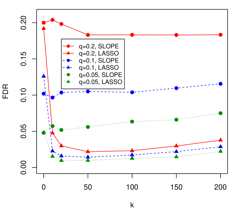
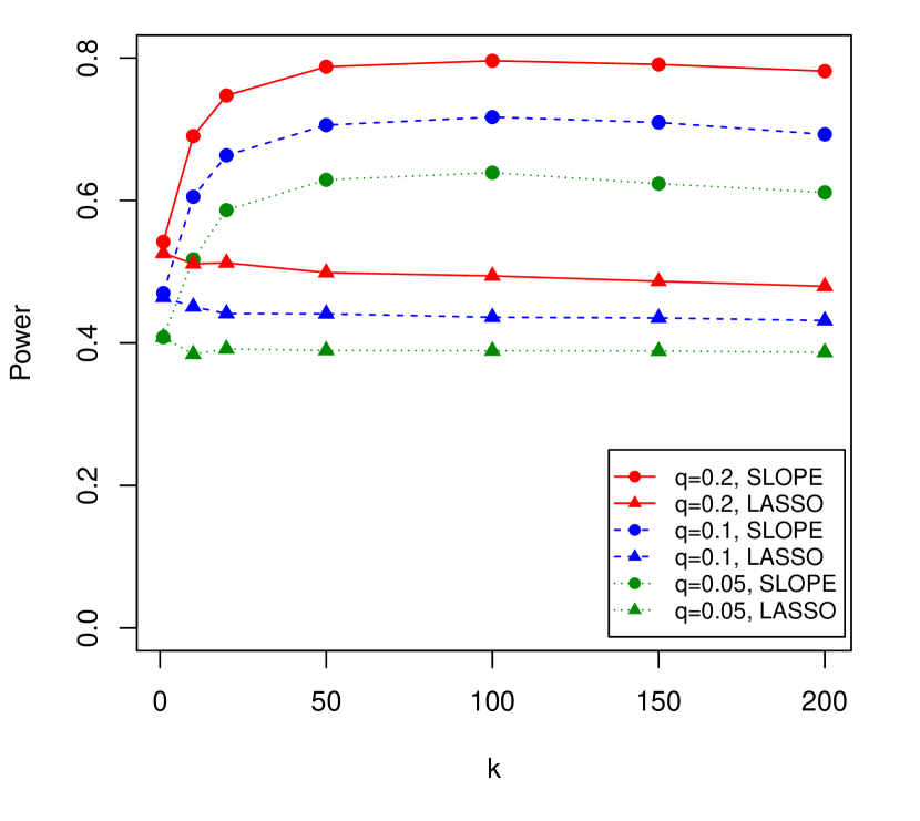
Figure 6: FDR and power of SLOPE and of the lasso with $\lambda=\lambda_{\text{BH}}(1)=\lambda_{\text{BHc}}(1)$; $n=p=5000$, $\beta_{i}=\sqrt{2\log p}$ for $i=1,\ldots,k$.

5 Numerical Examples

5.1 Multiple testing

5.1.1 Genome wide association studies

In this section we report the results of simulations inspired by the genome-wide search for influential genes. In this case the regressor variables can take on only three values according to the genotype of a genetic marker. In details, $X=0$ if a given individual has two copies of a reference allele at a given marker, $X=2$ if she has two copies of a variant allele, and $X=1$ if this individual is heterozygous, i.e., has one copy of a reference and one copy of a variant allele. For this study we used simulated data relating to 1,000 individuals from the admixture of the African-American (ASW) and European (CEU) populations, based on the HapMap [18] genotype data. The details of the simulation of the admixture are described in [12]. The original data set contains 482,298 markers (locations on the genome) in which genotypes at neighboring markers are usually strongly correlated. To avoid ambiguities related to the definition of the true and false positives we extensively pruned the design matrix, leaving only 892 markers distributed over all chromosomes. In this final data set the maximal pairwise correlation between those genotypes at different marker locations is equal to 0.2. The columns of the design matrix are further standardized, so that each variable has zero mean and variance equal to one (in other words, the $\ell_{2}$ norm of each column is equal to one). The design matrix used in our simulation study is available at http://www-stat.stanford.edu/~candes/SortedL1/Gen.txt. Following the arguments from Section 4.3, the weights $w_{k}$ for $\lambda_{\text{BHc}}$ are

$$w_{k}=\frac{1}{k}\mathbb{E}\|(X_{\mathcal{S}}^{\prime}X_{\mathcal{S}})^{-1}X^{\prime}_{\mathcal{S}}X_{i}\|_{2}^{2},$$ (5.1)

where the expectation is taken over all subsets $\mathcal{S}\subseteq\{1,\ldots,p\}$ with $|\mathcal{S}|=k$ and $i\notin\mathcal{S}$. Here, we substitute this expectation with an average over 5000 random samples when $k<300$ and 2500 random samples for larger $k$. The weights are estimated for $k\in\{1,6,11,\ldots,296\}$ and $k\in\{300,310,320,\ldots,890\}$ and we use linear interpolation to estimate the remaining values. As seen in Figure 7(a), for small $k$ the estimated weights are slightly larger than the corresponding weights for the Gaussian design matrix. In the most relevant region where $k<50$ they slightly decrease with $k$. When using this selection of weights the critical points $k^{\star}$ for $q\in\{0.05,0.1,0.2\}$ are equal to $15$, $32$ and $67$.

In our study, we compare the performance of SLOPE with two other approaches that are sometimes used to control the false discovery rate. The first approach is often used in real Genome Wide Association Studies (GWAS) and operates as follows: first, carry out simple regression (or marginal correlation) tests at each marker and then use the Benjamini-Hochberg procedure to adjust for multiplicity (and hopefully control the overall FDR). The second approach uses the Benjamini-Hochberg procedure with $p$-values obtained by testing the significance of individual predictors within the full regression model with 892 regressors. We assume Gaussian errors and according to Theorem 1.3 in [10], applying the BHq procedure with $q={q_{0}}/S_{p}$, $S_{p}=\sum_{i=1}^{p}{1}/{i}$, controls the FDR at level $q_{0}$. In our context, the logarithmic factor makes the procedure too conservative and in our comparison, we shall use the BHq procedure with $q$ being equal to the FDR level we aim to obtain. The reader will observe that in our experiments, this choice keeps the FDR around or below the nominal level $q$ (had we opted for $q/S_{p}$, we would have had an FDR well below the nominal level and essentially no power).

The trait or response is simulated according to the linear model (1.1), where $z$ is a 1,000-dimensional vector with i.i.d. $\mathcal{N}(0,1)$ entries. The number $k$ of nonzero elements in the regression coefficient vector $\beta$ varies between 0 and 40. For each $k$, we report the values of the FDR and power by averaging false discovery proportions over 500 replicates. In each replicate, we generate a new noise vector and a regression coefficient vector at the appropriate sparsity level by selecting locations of the nonzero coefficients uniformly at random. The amplitudes are all equal to $5\sqrt{2\log p}$ (strong signals) or $\sqrt{2\log p}$ (weak signals).

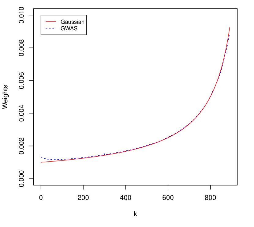
(a) Weights $w_{k}$ as a function of $k$.

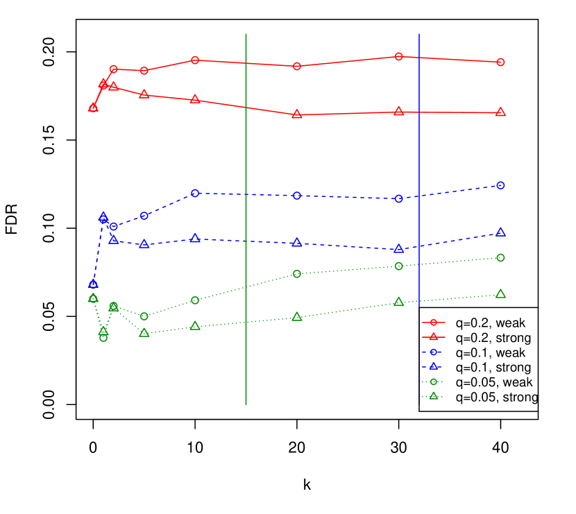
(b) FDR as a function of $k$.

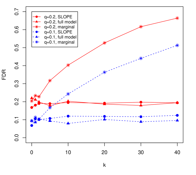
(c) FDR as a function of $k$.

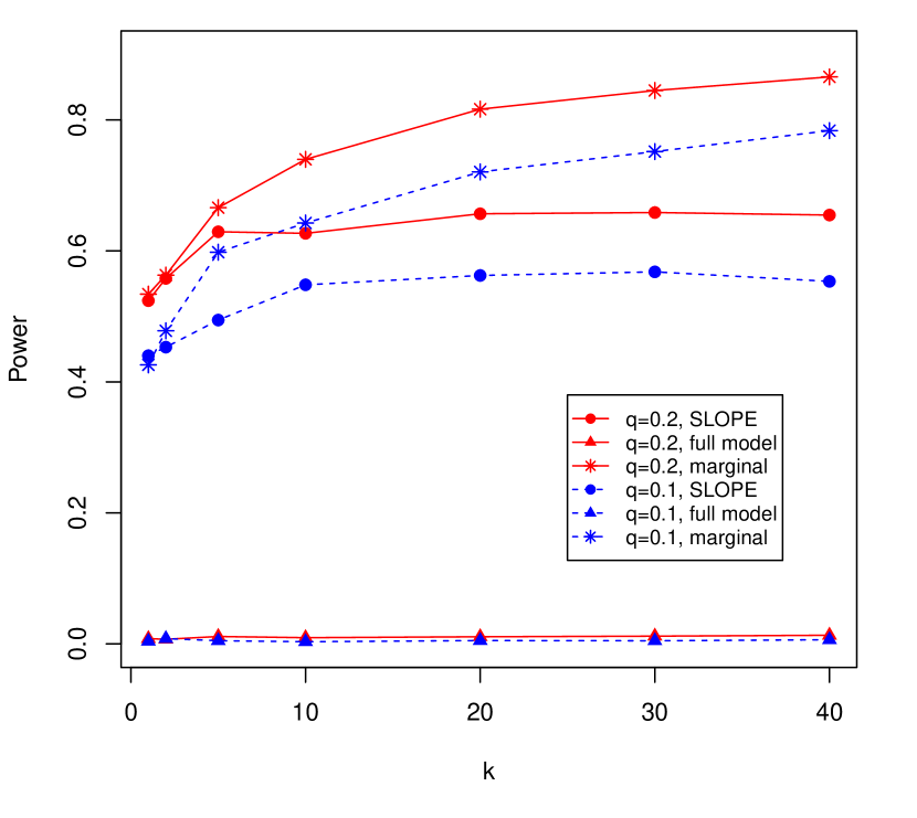
(d) Power as a function of $k$.

Figure 7: Simulation results for the GWAS inspired examples. The weights for SLOPE are shown in (a). In (b), the vertical lines represent the locations of the critical points for $q=0.05$ and $q=0.1$. As mentioned in the text weak (resp. strong) signals have amplitudes equal to $\sqrt{2\log p}$ (resp. $5\sqrt{2\log p}$). Plots (c) and (d) show the FDR and power of the different methods operating at the nominal level $q=0.1$ in the case of weak signals.

As observed in Figure 7(b), when the signals are strong SLOPE keeps the FDR close to or below the nominal level whenever the number of non-nulls is less or equal to the value $k(n,p,q)$ of the critical point. As in the case of Gaussian matrices, FDR control is more difficult when signals have a moderate amplitude; even in this case, however, the FDR is kept close to the nominal level as long as $k$ is below the critical point.

Figures 7(c) and 7(d) compare the FDR and the power of the three different approaches when effects are weak ($\beta=\sqrt{2\log p}$). In Figure 7(c) we observe that the method based on marginal tests completely fails to control FDR when the number of true regressors exceeds 10. For $k=10$ this method has a FDR two times larger than the nominal level. For $k=40$, the FDR exceeds 50% meaning that the ‘marginal method’ carried out at the nominal FDR level $q=0.1$ detects more false than true regressors. This behavior can be easily explained by observing that univariate models are not exact: in a univariate least-squares model, we estimate the projection of the full model on a simpler model with one regressor. Even a small sample correlation between the true regressor $X_{1}$ and some other variable $X_{2}$ will make the expected value of the response variable dependent on $X_{2}$. In passing, this phenomenon illustrates a basic problem related to the application of marginal tests in the context of GWAS; marginal tests yield far too many false regressors even in situations where correlations between the columns of the design matrix are rather small. The method based on the tests within the full regression model behaves in a completely different way. It controls the FDR at the assumed level but has no detection power. This can be explained by observing that least squares estimates of regression coefficients have a large standard deviation when $n$ is comparable to $p$. In comparison, SLOPE performs very well. When $k\leq 40$, the FDR is kept close to the nominal level and the method has a large power, especially when one considers that the magnitude of the simulated signals are comparable to the upper quantiles of the noise distribution.

5.1.2 Multiple mean testing from correlated statistics

We now illustrate the properties of our method as applied to a classical multiple testing problem with correlated test statistics. Imagine that we perform $p=1,000$ tests in each of 5 different laboratories and that there is a significant random laboratory effect. The test statistics can be modeled as

$$y_{i,j}=\mu_{i}+\tau_{j}+z_{i,j},\quad 1\leq i\leq 1000,\,\,1\leq j\leq 5,$$

where the laboratory effects $\tau_{j}$ are i.i.d. mean-zero Gaussian random variables as are the errors $z_{i,j}$. The random lab effects are independent from the $z$’s. We wish to test whether $H_{j}:\mu_{j}=0$ versus a two-sided alternative. In order to do this, imagine averaging the scores over all five labs, which gives

$$\bar{y}_{i}=\mu_{i}+\bar{\tau}+\bar{z}_{i},\quad 1\leq i\leq n.$$

We assume that things are normalized so that $\operatorname{Var}(\bar{y}_{i})=1$, the vector $\bar{y}\sim\mathcal{N}(0,\Sigma)$ where $\Sigma_{i,i}=1$ and $\Sigma_{i,j}=\rho>0$ for $i\neq j$. Below, we shall work with $\rho=0.5$.

Our problem is to test the means of a multivariate Gaussian vector with equicorrelated entries. One possible approach is to use the Benjamini-Hochberg procedure, that is we order $|\bar{y}|_{(1)}\geq|\bar{y}|_{(2)}\geq\ldots\geq|\bar{y}|_{(p)}$ and apply the step-up procedure with critical values equal to $\Phi^{-1}(1-iq/2p)$. Because the statistics are correlated we would use a conservative level equal to $q/S_{p}$ as suggested in [10, Theorem 1.3]. However, this is really too conservative and, therefore, in our comparisons we selected $q$ to be the FDR level we wish to obtain. (The reader will again observe that in our experiments, this choice keeps the FDR below the nominal level $q$. Had we opted for $q/S_{p}$, we would have had an FDR well below the nominal level and essentially no power).

Another possible approach is to ‘whiten the noise’ and express our multiple testing problem in the form of a regression equation

$$\tilde{y}=\Sigma^{-1/2}\bar{y}=\Sigma^{-1/2}\mu+\epsilon,$$ (5.2)

where $\epsilon\sim\mathcal{N}(0,I_{p})$, and use model selection tools for identifying the nonzero elements of $\mu$.

Interestingly, while the matrix $\Sigma$ is far from being diagonal, $\Sigma^{-1/2}$ is diagonally dominant. Specifically, $\Sigma^{-1/2}_{i,i}=1.4128$ and $\Sigma^{-1/2}_{i,j}=-0.0014$ for $i\neq j$. This makes our multiple testing problem well suited for the application of SLOPE with the original $\lambda_{\text{BH}}$ values. Hence, we work with (5.2) in which we normalize $\Sigma^{-1/2}$ as to have unit norm columns.

For the purpose of this study we simulate a sequence of sparse multiple testing problems, with the number $k$ of nonzero $\mu_{i}$ varying between 0 and 80. With $\Sigma^{-1/2}$ normalized as above, all the nonzero means are equal to $\sqrt{2\log p}$ so that $\tilde{y}\sim\mathcal{N}(\tilde{\Sigma}^{-1/2}\mu,I_{p})$ in which $\tilde{\Sigma}^{-1/2}$ has unit normed columns. The magnitude of true effects was chosen so as to obtain a moderate power of their detection. For each sparsity level $k$, the results are averaged over 500 independent replicates.

In Figures 8 and 9 we present the summary of our simulation study, which reveals that SLOPE solves the multiple testing problem in a much better fashion than the BHq procedure applied to marginal test statistics. In our setting, the BHq procedure is too conservative as it keeps the FDR below the nominal level. Moreover, as observed in Figure 9, when $q=0.1$ and $k=50$, in approximately 75% of the cases the observed False Dicovery Proportion (FDP) is equal to 0, while in the remaining 25% of the cases, it takes values which are distributed over the whole interval (0,1). FDP taking the value zero in a majority of the cases is not welcome since it is related to a low power. To be sure, in approximately 35% of all cases BHq did not make any rejections (i.e., $R=0$). Conditional on $R>0$, the mean of FDP is equal to 0.22 with a standard deviation of 0.28, which clearly shows that the observed FDP is typically far away from the nominal value of $q=0.1$. Because of this behavior, the applicability of the BHq procedure under this correlation structure is in question since for any given realization, the FDP may be very different from its targeted expected value. In comparison to BHq, SLOPE offers a more predictable FDR and substantially larger and more predictable True Positive Proportion (TPP, fraction of correctly identified true signals), compare the spread of the histograms in Figure 9.

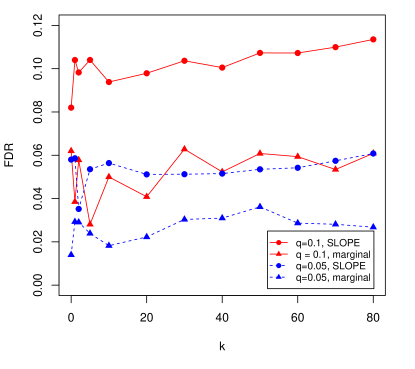
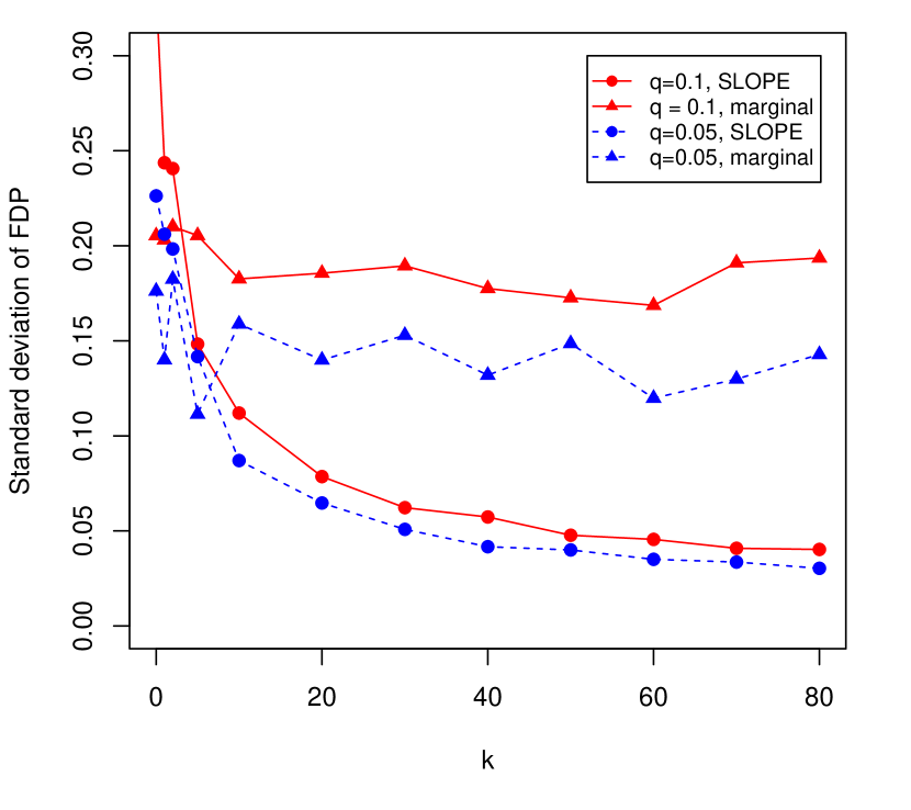
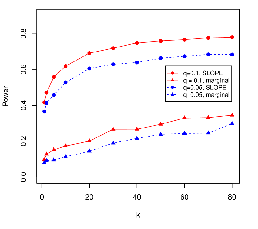
Figure 8: Simulation results for testing multiple means from correlated statistics. (a) FDR levels for SLOPE and marginal tests as a function of $k$. (b) Variability of the false discovery proportions for both methods. (c) Power plot.

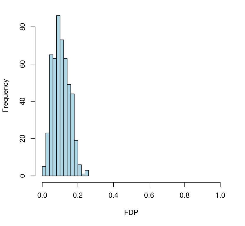
(a) Observed FDP for SLOPE.

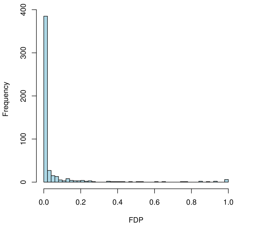
(b) Observed FDP for marginal test.

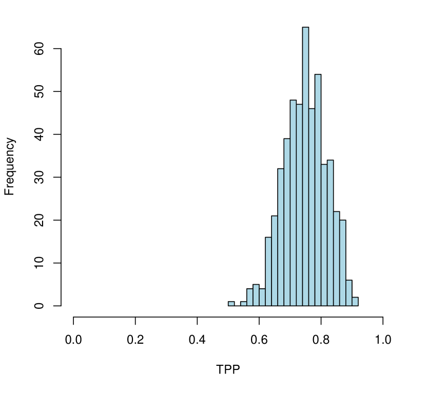
(c) Observed TPP for SLOPE.

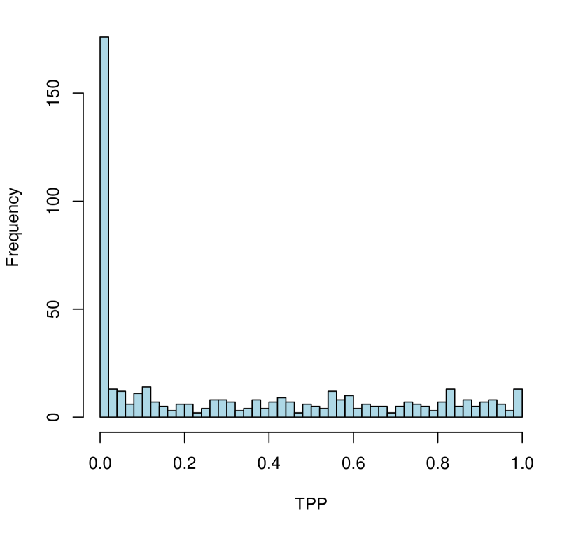
(d) Observed TPP for marginal test.

Figure 9: Testing example with $q=0.1$ and $k=50$.

5.2 High-dimensional compressive sensing examples

The experiments presented so far all used an $n\times p$ matrix $X$ with $n\approx p$. In this section we consider matrices with $n\ll p$. Such matrices are used in compressive sensing [15, 16, 19] to acquire linear measurements of signals $\beta$ that are either sparse or can be sparsely represented in a suitable basis. In particular, we observe $y=X\beta+z$, where $z$ is an additive noise term. We assume that $z\sim\mathcal{N}(0,\sigma^{2}I)$, and that $\sigma$ is known. Despite the underdetermined nature of the problem, there is now a large volume of theoretical work in the field of compressed sensing that shows that accurate reconstructions of $\beta$ can nevertheless be obtained using $\ell_{1}$-based algorithms such as the lasso.

The goal of our simulations is to compare the performance of the lasso and SLOPE in this setting, and to evaluate their sensitivity with respect to the regularizing parameters $\lambda$ and $q$, respectively.

5.2.1 Sparse signals

As a first experiment we generate an $n\times p$ matrix $X$ by taking the $p\times p$ matrix corresponding to the one-dimensional discrete cosine transformation (DCT-II) for signals of length $p$, and randomly selecting $n$ different rows in such a way that the first row is always included. We then scale the matrix by a factor $\sqrt{p/n}$ to obtain approximately unit-norm columns. Note that including the first row of the DCT matrix, all of whose entries are identical, ensures that we have information about the mean of the signal. Throughout this section we use a fixed instance of $X$ with $n=p/2$ and $p=262,\!144$.

The signals $\beta$ are constructed as follows. First a random support set $\mathcal{S}\subset\{1,\ldots,p\}$ of cardinality $k$ is drawn uniformly at random. We then set the off-support entries to zero, i.e., $\beta_{i}=0$ for all $i\not\in\mathcal{S}$, and choose the remaining $k$ entries $\beta_{i}$ with $i\in\mathcal{S}$ according to one of six signal classes:

1. Random Gaussian entries: $\beta_{i}\sim\mathcal{N}(0,\sigma^{2})$ with $\sigma=2\sqrt{2\log p}$.

2. Random Gaussian entries: $\beta_{i}\sim\mathcal{N}(0,\sigma^{2})$ with $\sigma=3\sqrt{2\log p}$.

3. Constant values: $\beta_{i}=1.2\sqrt{2\log{p}}$.

4. Linearly decreasing from $1.2\sqrt{2\log p}$ to $0.6\sqrt{2\log p}$.

5. Linearly decreasing from $1.5\sqrt{2\log p}$ to $0.5\sqrt{2\log p}$.

6. Linearly decreasing from $4.5\sqrt{2\log p}$ to $1.5\sqrt{2\log p}$.

In the last three classes, the linear ranges are randomly permuted before assigning their values to the respective entries in $\beta$. As a final signal class, $\beta$ is chosen to be a random permutation of the following dense vector $v$:

1. Exponentially decaying entries: $v_{i}=1.2\sqrt{2\log{p}}\left(i/k\right)^{-1.2}$.

We consider nine sparsity levels $k$: 1, 5, 10, 50, 100, 500, 1000, 1%, and 5%, where the percentages are relative to $p$ (thus giving $k=2,621$ and $k=13,017$, respectively for the last two choices). The noise vector $z$ is always generated from the multivariate normal $\mathcal{N}(0,1)$ distribution.

The $k$ largest entries in $\beta$ are designed to lie around the critical level with respect to the noise. Especially for highly sparse $\beta$, this means that the power and FDR obtained with any of the methods under consideration depends strongly on the exact combination of $\beta$ and $z$. To avoid large fluctuations in individual results, we therefore report the result as averaged over 100 random signal and noise instances for $k\leq 50$, and over 50 instances for $k=100$ and $k=500$. For larger $k$ individual instances were found to be sufficient.

The mean square error of the estimated regression coefficients, $\hat{\beta}$ is defined as

$$\mathrm{MSE}=\frac{1}{p}\sum_{i=1}^{p}\operatorname{\mathbb{E}}(\hat{\beta}_{i}-\beta_{i})^{2}.$$

In our numerical experiments we work with estimated MSE values in which the expectation is replaced by the mean over a number of realizations of $\beta$ and the corresponding $\hat{\beta}$. For convenience we refer to this as the MSE, but it should be kept in mind that this is only an estimation of the actual MSE.

In preliminary experiments we observed that under sparse scenarios the bias due to the shrinkage of regression coefficients has a deteriorating influence on the MSE of both the lasso and SLOPE estimates. We therefore suggest to use a debiasing step in which the results from the lasso or SLOPE are used only to identify the nonzero regression coefficients. The final estimation of their values is then performed with the classical method of least squares on that support. Having too many incorrect entries in the support distorts the estimates of the true nonzero regression coefficients and it is thus important to maintain a low FDR. At the same time we need a large power: omitting entries from the support not only leads to zero estimates for those coefficients, but also distorts the estimates of those coefficients belonging to the support. Figure 10 shows the effect the debiasing step has on the (estimated) MSE. (In the consecutive graphs we report only the results for the debiased version of the lasso and SLOPE). In all but the least sparse cases, the minimum MSE with debiasing is always lower than the best MSE obtained without it. The figure also shows the dependency of the MSE on $\lambda$ for the lasso and $q$ for SLOPE. The optimal choice of $\lambda$ for the lasso was found to shift considerably over the various problem settings. By contrast, the optimal $q$ for SLOPE remained fairly constant throughout. Moreover, in many cases, using a fixed value of $q=0.02$ gives MSE values that are close to, and sometimes even below, the lowest level obtained using the lasso.

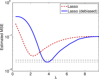
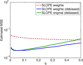
(a)	(b)
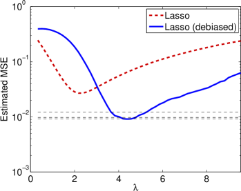
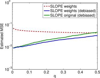
(c)	(d)
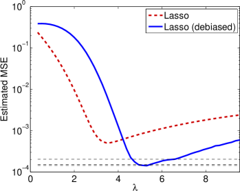
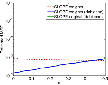
(e)	(f)

Figure 10: Estimated mean square error value for $\hat{\beta}$ before and after debiasing for (a,b) signal class $5$, $k=1000$, (c,d) signal class $2$, $k=1000$, and (e,f) signal class $2$, $k=10$. The plots on the left show the results obtained using the lasso algorithm, along with horizontal lines indicating the performance of SLOPE with from bottom to top: the optimal value of $q$; $q=0.02$; and the worst value of $q$ in the interval $0.01$ to $0.1$. The plots on the right show the (debiased) results of SLOPE with and without adaptive weights.

Figure 11 shows the power and FDR results obtained for signals of classes 3 and 5 using the lasso with various $\lambda$ values. The different FDR curves in the plot correspond to increasing levels of sparsity (fewer nonzeros) from left to right. For fixed $\lambda$ values, the power for a fixed signal class is nearly independent of the sparsity level. The FDR, on the other hand, increases significantly with sparsity.

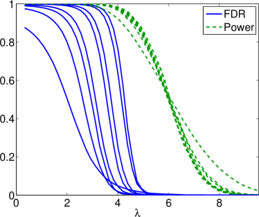
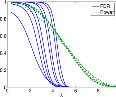
(a)	(b)

Figure 11: FDR and power results obtained using lasso for different sparsity levels and (a) signals of class 3, and (b) signal of class 5. The FDR curves from the right to the left correspond to decreasing sparsity (more nonzero entries in $\beta$): $k=1,5,10,50,100,500,1000,2621$, and $13,017$.

The FDR and power results obtained with SLOPE are shown in Figure 12. Here, the results are grouped by sparsity level, and the different curves in each plot correspond to the seven different signal classes. The FDR curves for each sparsity level are very similar. The power levels differ quite a bit depending on how ‘difficult’ the signal is to recover. In plots (a)–(c) the results between SLOPE with fixed and adapted weights (see Section 4.3) are almost identical. In plot (d), however, the FDR of SLOPE with adapted weights is much lower, at the expense of some of the power. Importantly, it can be seen that for a wide range of sparsity levels, the adaptive version keeps FDR very close to the nominal level indicated by the gray dashed line.

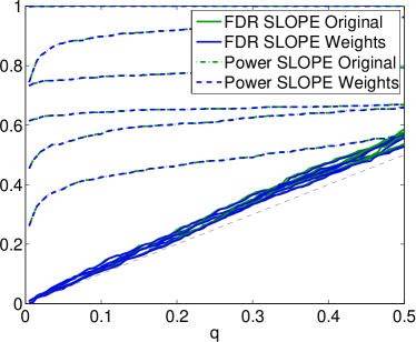
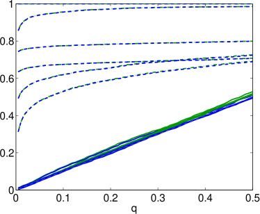
(a) $k=10$	(b) $k=50$
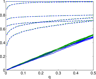
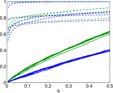
(c) $k=100$	(d) $k=1\%$

Figure 12: Power and FDR results obtained using SLOPE. Each plots shows the results for all seven signal classes for a fixed sparsity level. At $q=0.1$ the lines from top to bottom correspond to classes 4,5,1,2,3, and 6 for plots (a)–(c), and to 1,4,5,2,3, and 6 for plot (d). The dashed gray line indicates the nominal FDR level.

We mentioned above that the optimal parameter choice for SLOPE is much more stable than that for the lasso. Because the optimal value depends on the problem it would be much more convenient to work with a fixed $\lambda$ or $q$. In the following experiment we fix the parameter for each method and then determine over all problem instances the maximum ratio between the optimal (two-norm) misfit over all parameters (for both lasso and SLOPE) and the misfit obtained with the given parameter choice. Table 2 summarizes the results. It can be seen that the optimal parameter choice for a series of signals from the different classes generated with a fixed sparsity level changes rapidly for lasso (between $\lambda=3.46$ and $\lambda=5.49$), whereas it remains fairly constant for SLOPE (between $q=0.01$ and $q=0.04$. Importantly, the maximum relative misfit for lasso over all problem instances varies tremendously for each of the $\lambda$ values in the given range. For SLOPE, the same maximum relative misfit changes slightly over the given parameter range for $q$, but far more moderately. Finally, the results obtained with the parameter that minimizes the maximum relative misfit over all problem instances are much better for SLOPE.

$k$		1	5	10	50	100	500	1000	1%	5%	Max.
Lasso	$\lambda=3.28$	3100.9	2118.3	1698.5	705.5	477.9	183.8	123.0	62.1	24.8	3100.9
	$\lambda=3.46$	2316.3	1571.0	1256.0	510.8	342.4	126.9	83.7	40.2	18.1	2316.3
	$\lambda=3.83$	1199.0	790.8	636.2	240.9	147.4	51.8	33.2	16.3	18.7	1199.0
	$\lambda=4.02$	827.5	540.7	430.2	154.3	90.7	28.3	18.1	11.5	25.4	827.5
	$\lambda=4.20$	546.8	352.5	281.5	91.7	52.2	14.4	12.4	19.1	38.2	546.8
	$\lambda=4.57$	200.9	116.2	94.4	24.2	12.9	23.1	36.4	45.7	64.0	200.9
	$\lambda=4.75$	113.1	56.4	48.6	11.7	21.5	37.2	57.9	65.6	77.3	113.1
	$\lambda=4.94$	53.5	33.9	22.0	23.7	39.9	53.8	75.6	84.0	90.9	90.9
	$\lambda=5.31$	20.0	28.3	27.4	58.7	77.2	92.0	128.0	122.0	116.6	128.0
	$\lambda=5.49$	11.3	39.4	38.7	74.5	94.3	111.9	149.2	141.2	127.9	149.2
SLOPE	$q=0.01$	14.9	27.1	17.3	13.1	14.3	14.7	16.8	20.3	38.6	38.6
	$q=0.02$	11.5	17.8	24.0	20.1	17.8	15.4	14.2	11.6	24.0	24.0
	$q=0.03$	17.9	29.8	31.2	28.0	24.6	22.1	23.7	15.2	19.7	31.2
	$q=0.04$	17.9	36.6	45.0	36.4	32.9	29.2	29.5	19.1	16.5	45.0
	$q=0.10$	47.9	66.6	89.6	77.5	69.0	63.3	54.8	38.9	19.3	89.6
	$q=0.12$	52.7	82.2	101.0	89.1	78.5	72.2	65.4	46.0	22.2	101.0
	$q=0.15$	78.9	102.0	123.7	106.7	94.4	85.4	77.2	54.8	25.8	123.7

Table 2: Entries in the table give the maximum ratio $(||\hat{b}-b||_{2}/||\hat{b}_{\mathrm{opt}}-b||_{2})-1$ in percent over all signal types with the given sparsity. Here $b$ is an instance of $\beta$; $\hat{b}$ is the corresponding estimate obtained using lasso and SLOPE with the given parameter value; and $\hat{b}_{\mathrm{opt}}$ is the estimate with the lowest two-norm misfit over all parameters and both methods. The entries in red show the lowest ratio obtained with either method for the given sparsity level. The entries in blue correspond to the parameter choice that gives the lowest maximum ratio over all problems.

5.2.2 Phantom

As a more concrete application of the methods, we now discuss the results for the reconstruction of phantom data from subsampled discrete-cosine measurements. Denoting by $x\in\mathbb{R}^{p}$ the vectorized version of a phantom with $p$ pixel values, we observe $y=RDx$, where $R$ is a restriction operator and $D$ is a two-dimensional discrete-cosine transformation. Direct reconstruction of the signal from $y$ is difficult because $x$ is not sparse. However, when expressed in a suitable wavelet basis the coefficients become highly compressible. Using the two-dimensional Haar wavelet transformation $H$, we can write $\beta=Hx$, or by orthogonality of $H$, $x=H^{T}\beta$. Combining this we get to the desired setting $y=X\beta$ with $X:=RDH^{T}$, and $\beta$ approximately sparse. Once the estimated $\hat{\beta}$ is known we can obtain the corresponding signal estimation using $\hat{x}=H^{T}\hat{\beta}$. Note that due to orthogonality of $H$ we have that $\|{x-\hat{x}}\|_{2}=\|{\beta-\hat{\beta}}\|_{2}$, and it therefore suffices to report only the MSE values for $\hat{\beta}$.

For our experiments we generated a test phantom by discretizing the analytical phantoms described in Guerquin-Kern, et al. [25] and available on the accompanying website. The resulting $2048\times 2048$ image, illustrated in Figure 13, is then vectorized to obtain $x$ with $p=2048^{2}$. We obtain $\beta$ using the two-dimensional Haar transformation implemented in the Rice wavelet toolbox [5] and interfaced though the Spot linear operator toolbox [37]. As summarized in Table 3, we consider two subsampling levels: one with $n=p/2$, the other with $n=p/5$. For each of the subsampling levels we choose a number of different noise levels based on a target sparsity level $k$. In particular, we choose $k=\lceil\gamma p/10^{4}\rceil$, and then set $\sigma=|\beta|_{[k]}/(1.2\sqrt{2\log p})$. The values of $\gamma$ and the resulting signal-to-noise ratios (${\left\lVert{X\beta}\right\rVert}_{2}/{\left\lVert{X\beta-y}\right\rVert}$) for each problem setting are listed in Table 3.

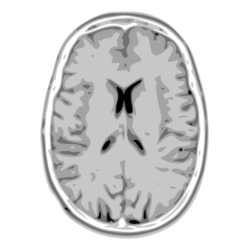
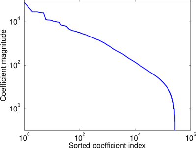
(a)	(b)

Figure 13: Illustration of (a) a discretized version of the continuous phantom data, shown with inverted grayscale, and (b) the magnitudes of the Haar wavelet coefficients in decreasing order.

Problem	1	2	3	4	5	6	7	8
$n/p$	0.5	0.5	0.5	0.5	0.2	0.2	0.2	0.2
$\gamma$	30	20	10	5	500	50	20	10
SNR	5.97	4.25	2.39	1.43	411.7	19.5	9.10	5.12

Table 3: Different problem configurations for phantom reconstruction with $p=2048^{2}$. The number of observations $n$ is prescribed by the given ratios $n/p$. The noise level $\sigma$ is set to $|\beta|_{[k]}/(1.2\sqrt{2\log{p}})$ with $k=\lceil\gamma p/10^{4}\rceil$.

As in the previous section we are interested in the sensitivity of the results with respect to the parameter choice, as well as in the determination of a parameter value that does well over a wide range of problems. We therefore started by running the lasso and SLOPE algorithms with various choices of $\lambda$ and $q$, respectively. The resulting relative two-norm misfit values are summarized in Table 4. The minimum MSE value obtained using the lasso are typically slightly smaller than those obtained using SLOPE, except for problems 3 and 4. On the other hand, the relative misfit values obtained over the given parameter ranges vary more than those for SLOPE.

Problem idx.		1	2	3	4	5	6	7	8
Lasso	$\lambda=3.50$	8.589	10.544	14.627	19.474	2.018	7.821	11.742	15.848
	$\lambda=3.75$	8.570	10.415	14.158	18.324	2.010	7.723	11.390	15.098
	$\lambda=4.00$	8.667	10.513	14.101	17.884	2.000	7.670	11.198	14.720
	$\lambda=4.25$	8.851	10.683	14.251	17.995	1.992	7.669	11.163	14.635
	$\lambda=4.50$	9.067	10.904	14.525	18.222	1.985	7.694	11.234	14.764
	$\lambda=4.75$	9.300	11.140	14.820	18.614	1.980	7.769	11.384	14.966
	$\lambda=5.00$	9.536	11.388	15.092	19.042	1.979	7.884	11.592	15.202
SLOPE	$q=0.01$	8.837	10.702	14.364	18.211	1.988	7.724	11.289	14.836
	$q=0.02$	8.694	10.569	14.201	18.037	1.994	7.679	11.195	14.711
	$q=0.03$	8.627	10.495	14.118	17.948	1.999	7.678	11.178	14.658
	$q=0.04$	8.593	10.449	14.100	17.876	2.002	7.677	11.179	14.651
	$q=0.05$	8.580	10.430	14.089	17.876	2.006	7.678	11.190	14.670
	$q=0.10$	8.598	10.487	14.188	18.061	2.017	7.695	11.258	14.815
	$q=0.12$	8.635	10.542	14.274	18.160	2.021	7.707	11.304	14.916

Table 4: Relative misfit values $||\hat{b}-b||_{2}/||b||_{2}$ (scaled by 100 for display purposes) for different phantom test problem instances with $b=\beta$ and its corresponding estimate $\hat{b}$, using lasso and SLOPE. The highlighted entries indicate the lowest misfit values obtained on a given problem using each of the two methods. Not shown is the minimum relative misfit of $1.971$ for problem 5 obtained using the lasso using $\lambda=6.0$.

Table 5 shows the percentage difference of each estimate to the lowest two-norm misfit obtained with either of the two methods for each problem. The results obtained with the parameters that minimize the maximum difference over all problem instances are highlighted. In this case, using the given parameters for each methods gives a similar maximum difference of approximately $1.4\%$. This value is again very sensitive to the choice of $\lambda$ for the lasso but remains much lower for the given parameter choices for SLOPE. More interestingly perhaps is to compare the results in Tables 2 and 5. Choosing the best fixed value for the lasso obtained for the DCT problems ($\lambda=4.94$) and applying this to the phantom problem gives a maximum difference close to $10\%$. This effect is even more pronounced when using the best parameter choice ($\lambda=4.00$) from the phantom experiment and applying it to the DCT problems. In that case it leads to deviations of up to $800\%$ relative to the best. For SLOPE the differences are minor: applying the DCT-optimal parameter $q=0.02$ gives a maximum deviation of $1.474\%$ instead of the best $1.410\%$ on the phantom problems. Vice versa, applying the optimal parameter for the phantom, $q=0.03$ to the DCT problems gives a maximum deviation of $31.2\%$ compared to $24.0\%$ for the best.

Problem idx.		1	2	3	4	5	6	7	8	Max.
Lasso	$\lambda=3.50$	0.232	1.237	3.817	8.940	2.378	1.989	5.190	8.287	8.940
	$\lambda=3.75$	0.000	0.000	0.489	2.504	1.952	0.702	2.041	3.163	3.163
	$\lambda=4.00$	1.140	0.938	0.085	0.045	1.475	0.011	0.315	0.581	1.475
	$\lambda=4.25$	3.284	2.574	1.148	0.667	1.038	0.000	0.000	0.000	3.284
	$\lambda=4.50$	5.806	4.690	3.091	1.936	0.715	0.330	0.638	0.879	5.806
	$\lambda=4.75$	8.527	6.956	5.189	4.131	0.443	1.300	1.985	2.259	8.527
	$\lambda=5.00$	11.281	9.340	7.118	6.525	0.372	2.804	3.850	3.869	11.281
SLOPE	$q=0.01$	3.123	2.758	1.949	1.873	0.866	0.722	1.132	1.370	3.123
	$q=0.02$	1.449	1.474	0.795	0.903	1.134	0.130	0.293	0.519	1.474
	$q=0.03$	0.668	0.770	0.202	0.406	1.410	0.126	0.138	0.153	1.410
	$q=0.04$	0.270	0.327	0.074	0.001	1.585	0.110	0.145	0.106	1.585
	$q=0.05$	0.117	0.140	0.000	0.000	1.743	0.124	0.242	0.239	1.743
	$q=0.10$	0.326	0.687	0.697	1.033	2.346	0.338	0.859	1.231	2.346
	$q=0.12$	0.767	1.221	1.309	1.587	2.507	0.493	1.270	1.920	2.507

Table 5: Entries in the table give the maximum ratio $(||\hat{b}-b||_{2}/||\hat{b}_{\mathrm{opt}}-b||_{2})-1$ in percent for each problem and parameter setting. Here $b$ is an instance of $\beta$; $\hat{b}$ is the corresponding estimate obtained using lasso or SLOPE with the given parameter value; and $\hat{b}_{\mathrm{opt}}$ is the estimate with the lowest two-norm misfit over all parameters and both methods for a given problem. The entries in blue correspond to the parameter choice that gives the lowest maximum ratio over all problem instances.

5.2.3 Weights

When using SLOPE with the adaptive procedure (4.6) described in Section 4.3, we need to evaluate (5.1). For most matrices $X$, there is no closed-form solution to the above expectation, and numerical evaluation would be prohibitively expensive. However, we can get good approximations $\hat{w}_{k}$ of $w_{k}$ values by means of Monte-Carlo simulations. Even so, it remains computationally expensive to evaluate $w_{k}$ for all values $k\in[1,\min(n,p-1)]$. Our approach is to take 21 equidistant $k$ values within this interval, including the end points, and evaluate $\hat{w}_{k}$ at those points. The remaining weights are obtained using linear interpolation between the known values. For the first interval this linear approximation was found to be too crude, and we therefore sample $\hat{w}_{k}$ at an addition 19 equispaced points within the first interval, thus giving a total of 40 sampled points. The next question is how many random trials to take for each $\hat{w}_{k}$. Preliminary experiments showed that the variance in the sampled values reduces with increasing $k$, while the computation cost of evaluating one term in the expectation in (5.1) grows substantially. To avoid choosing a fixed number of samples and risk inaccurate estimations of $\hat{w}_{k}$ for small $k$, or waste time when evaluating $\hat{w}_{k}$ for large $k$, we used a dynamic sampling scheme. Starting with a small number of samples, we obtain an intermediate estimate $\hat{w}_{k}$. We then compute a reference approximation using the same number of samples, record the difference between the two values and update $\hat{w}_{k}$ to the average of the two. If the original difference was sufficiently small we terminate the algorithm, otherwise we double the number of samples and compute a new reference approximation, which is then again first compared to the current $\hat{w}_{k}$, and then merge into it, and so on. This process continues until the algorithm either terminates naturally, or when a pre-defined maximum sample size is reached.

In Figure 14 we plot the resulting weights obtained for three different types of matrices against $1/(n-k-1)$. The results in plot (a) are obtained for a $200\times 600$ matrix with entries sampled i.i.d. from the normal distribution, and with $\hat{w}_{k}$ for all $k\in[1,200]$ based on 10,000 samples. The blue line exactly follows the theoretical line for $w_{k}=1/(n-k-1)$, as derived in Section 4.3. Plots (b) show the results obtained for five instances of the the restricted DCT operator described in Section 5.2.1. We omit the value of $\hat{w}_{k}$ for $k=n$, which would otherwise distort the figure due to the choice of axes. In plot (c) we plot the weights for the matrices used in Section 5.2.2, along with additional instances with $n/p=0.3$ and $n/p=0.4$. The results in plots (b) and (c) are slightly below the reference line. The vertical dashed red lines in the plots indicate the maximum value of $k$ needed to evaluate $\lambda_{\text{BHc}}$ with $q=0.1$. In the DCT case we only need up to $k=5439$, and for DCT and Haar we need $k=14,322$ for $n/p=0.2$ and $k=95,472$ for $n/p=0.5$. In both cases this $k$ falls well within the first interval of the coarsely sampled grid. For a fixed $q$ it may therefore be possible to much further reduce the computational cost by evaluating successive $\hat{w}_{k}$ for increasing $k$ until the critical value is reached.

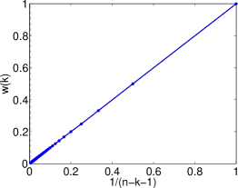
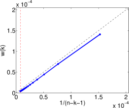
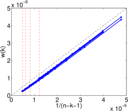
(a) Gaussian	(b) DCT	(c) DCT and Haar

Figure 14: Weights $w(k)$ plotted against $1/(n-k-1)$ for (a) a $200\times 600$ matrix with entries sampled i.i.d. from the normal distribution; (b) five instances of the restricted DCT matrix described in Section 5.2.2; and (c) matrices as described in Section 5.2.2 for $n/p$ ranging from 0.2 to 0.5. The vertical red lines indicate the weights needed to evaluate $\lambda_{\text{BHc}}$ for $q=0.1$.

6 Discussion

In this paper, we have shown that the sorted $\ell_{1}$ norm may be useful in statistical applications both for multiple hypothesis testing and for parameter estimation. In particular, we have demonstrated that the sorted $\ell_{1}$ norm can be optimized efficiently and established the correctness of SLOPE for FDR control under orthogonal designs. We also demonstrated via simulation studies that in some settings, SLOPE can keep the FDR at a reasonable level while offering increased power. Finally, SLOPE can be used to obtain accurate estimates in sparse or nearly sparse regression problems in the high-dimensional regime.

Our work suggests further research and we list a few open problems we find stimulating. First, our methods assume that we have knowledge of the noise standard deviation and it would be interesting to have access to methods that would not require this knowledge. A tantalizing perspective would be to design joint optimization schemes to simultaneously estimate the regression coefficients via the sorted $\ell_{1}$ norm and the noise level as in [34] for the lasso. Second, just as in the BHq procedure, where the test statistics are compared with fixed critical values, we have only considered in this paper fixed values of the regularizing sequence $\{\lambda_{i}\}$. It would be interesting to know whether it is possible to select such parameters in a data-driven fashion as to achieve desirable statistical properties. For the simpler lasso problem for instance, an important question is whether it is possible to select $\lambda$ on the lasso path as to control the FDR, see [26] for contemporary research related to this issue. Finally, we have demonstrated the limited ability of the lasso and SLOPE to control the FDR in general. It would be of great interest to know what kinds of positive theoretical results can be obtained in perhaps restricted settings.

Acknowledgements

E. C. is partially supported by AFOSR under grant FA9550-09-1-0643, by ONR under grant N00014-09-1-0258 and by a gift from the Broadcom Foundation. M. B. was supported by the Fulbright Scholarship and NSF grant NSF 1043204. E. v.d.B. was supported by National Science Foundation Grant DMS 0906812 (American Reinvestment and Recovery Act). W. S. is supported by a General Wang Yaowu SGF Fellowship. E. C. would like to thank Stephen Becker for all his help in integrating the sorted $\ell_{1}$ norm software into TFOCS, and Chiara Sabatti for fruitful discussions about this project. M. B. would like to thank David Donoho and David Siegmund for encouragement and Hatef Monajemi for helpful discussions. We are very grateful to Lucas Janson for suggesting the acronym SLOPE, and to Rina Foygel Barber for useful comments about an early version of the manuscript.

Appendix A Proofs of Intermediate Results

A.1 Proof of Proposition 1.1

Lemma A.1.

For all $w$ and $h$ in $\mathbb{R}^{n}$, we have

$$\sum_{i}w_{i}h_{i}\leq\sum_{i}|w|_{(i)}|h|_{(i)}.$$

Proof Since

$$\sum_{i}w_{i}h_{i}\leq\sum_{i}|w_{i}||h_{i}|,$$

it is sufficient to prove the claim for $w,h\geq 0$, which we now assume. Without loss of generality, suppose that $w_{1}\geq w_{2}\geq\ldots\geq w_{n}\geq 0$. Then

$$\sum_{i}w_{i}h_{i} =w_{n}(h_{1}+\ldots+h_{n})+(w_{n-1}-w_{n})(h_{1}+\ldots+h_{n-1})+\ldots+(w_{1}-w_{2})h_{1}$$

$$\leq w_{n}(h_{(1)}+\ldots+h_{(n)})+(w_{n-1}-w_{n})(h_{(1)}+\ldots+h_{(n-1)})+\ldots+(w_{1}-w_{2})h_{(1)}$$

$$=w_{n}h_{(n)}+w_{n-1}h_{(n-1)}+\ldots+w_{1}h_{(1)}$$

$$=\sum_{i}w_{(i)}h_{(i)},$$

which proves the claim.  

We are in position to prove Proposition 1.1. Suppose $w\in C_{\lambda}$, then Lemma A.1 gives

$$\sum_{i}w_{i}b_{i}\leq\sum_{i}|w|_{(i)}|b|_{(i)}=|b|_{(p)}(|w|_{(1)}+\ldots+|w|_{(p)})\\ +(|b|_{(p-1)}-|b|_{(p)})(|w|_{(1)}+\ldots+|w|_{(p-1)})+\ldots+(|b|_{(1)}-|b|_{(2)})|w|_{(1)}.$$

Next, membership to $C_{\lambda}$ allows to bound the right-hand side as

$$|b|_{(p)}(\lambda_{1}+\ldots+\lambda_{p})+(|b|_{(p-1)}-|b|_{(p)})(\lambda_{1}+\ldots+\lambda_{p-1})+\ldots+(|b|_{(1)}-|b|_{(2)})\lambda_{1}=\sum_{i}\lambda_{i}|b|_{(i)}.$$

This shows that $\sup_{w\in C_{\lambda}}\,\langle z,w\rangle\leq J_{\lambda}(b)$. For the equality, assume without loss of generality that $|b_{1}|\geq|b_{2}|\geq\ldots\geq|b_{p}|$ and take $w_{i}=\lambda_{i}\textrm{sgn}(b_{i})$. Then it is clear that $\langle w,b\rangle=\sum_{i}\lambda_{i}|b_{i}|=J_{\lambda}(b)$.

A.2 Proof of Proposition 1.2

Set $y=\tilde{y}$ for notational convenience, and following Section 2.1, assume without loss that $y_{1}\geq y_{2}\geq\ldots\geq y_{p}\geq 0$. Consider a feasible input $x_{1}\geq\ldots\geq x_{p}$ such that $x_{i_{\text{SU}}+1}>0$ and define $x^{\prime}$ as

$$x^{\prime}_{i}=\begin{cases}x_{i}&i\leq i_{\text{SU}}\\ 0&i>i_{\text{SU}}.\end{cases}$$

Then the difference in the objective functional is equal to

$$f(x)-f(x^{\prime})=\sum_{i>i_{\text{SU}}}\Bigl{\{}{\textstyle\frac{1}{2}}((y_{i}-x_{i})^{2}-y_{i}^{2})+\lambda_{i}x_{i}\Bigr{\}}=\sum_{i>i_{\text{SU}}}\Bigl{\{}{\textstyle\frac{1}{2}}x_{i}^{2}+(\lambda_{i}-y_{i})x_{i}\Bigr{\}}.$$

Since by definition $y_{i}\leq\lambda_{i}$ for $i>i_{\text{SU}}$, we see that $f(x)-f(x^{\prime})>0$. This shows that $i^{\star}\leq i_{\text{SU}}$.

We now argue that $\imath^{\star}\geq i_{\text{SD}}$. Take $x$ feasible as before obeying $x_{1}\geq\ldots x_{i_{0}}>0$ and $x_{i_{0}+1}=\ldots=x_{p}=0$ where $i_{0}<i_{\text{SD}}$. Define $x^{\prime}$ as

$$x^{\prime}_{i}=\begin{cases}x_{i}&i\leq i_{0}\\ h&i_{0}<i\leq i_{\text{SD}}\\ 0&i>i_{\text{SD}},\end{cases}$$

where $0<h\leq x_{i_{0}}$ is an appropriately small scalar. Observe that $x^{\prime}$ is feasible (i.e. is nonnegative and nonincreasing). The difference in the objective functional is equal to

$$f(x)-f(x^{\prime})=\sum_{i_{0}<i\leq i_{\text{SD}}}\Bigl{\{}{\textstyle\frac{1}{2}}(y_{i}^{2}-(y_{i}-h)^{2})-\lambda_{i}h\Bigr{\}}=\sum_{i_{0}<i\leq i_{\text{SD}}}\Bigl{\{}(y_{i}-\lambda_{i})h-{\textstyle\frac{1}{2}}h^{2}\Bigr{\}}.$$

Since by definition $y_{i}>\lambda_{i}$ for $i\leq i_{\text{SD}}$, we see that taking $h$ small enough gives $f(x)-f(x^{\prime})>0$, concluding the proof.

Appendix B Asymptotic Predictions of FDR Levels

Figures 1 and 2 in Section 1.6 display asymptotic predictions of FDR levels and it is now time to explain where they come from. These predictions can be heuristically derived by extending results from [32] and [6]. In a nutshell, [32] applies the replica method from statistical physics for computing the asymptotic performance of the lasso with Gaussian designs. In contrast, [6] rigorously proves asymptotic properties of the lasso solution in the same setting by studying an iterative scheme called approximate message passing (AMP) [21] inspired by belief-propagation on dense graphical models. Below, we follow [6].

B.1 Asymptotic properties of the lasso

Our predictions use the main result from [6, Theorem 1.5] that we shall state below with a bit less of generality. We begin with two definitions. First, a function $\varphi:\mathbb{R}^{2}\rightarrow\mathbb{R}$ is said to be pseudo-Lipschitz if there is a numerical constant $L$ such that for all $x,y\in\mathbb{R}^{2}$,

$$|\varphi(x)-\varphi(y)|\leq L(1+\|x\|_{\ell_{2}}+\|y\|_{\ell_{2}})\|x-y\|_{\ell_{2}}.$$

Second, for any $\delta>0$, we let $\alpha_{\text{min}}=\alpha_{\text{min}}(\delta)$ be the unique solution to

$$2(1+\alpha^{2})\Phi(-\alpha)-2\alpha\phi(\alpha)-\delta=0$$

if $\delta\leq 1$, and 0 otherwise.

Theorem B.1.

[6, Theorem 1.5] Consider the linear model with i.i.d. $\mathcal{N}(0,1)$ errors in which $X$ is an $n\times p$ matrix with i.i.d. $\mathcal{N}(0,1/n)$ entries. Suppose that the $\beta_{i}$’s are i.i.d. random variables, independent of $X$, and with positive variance (below, $\Theta$ is a random variable distributed as $\beta_{i}$). Then for any pseudo-Lipschitz function $\varphi$, the lasso solution $\hat{\beta}$ to (1.5) with fixed $\lambda$ obeys

$$\frac{1}{p}\sum_{i=1}^{p}\varphi(\hat{\beta}_{i},\beta_{i})\,\,\longrightarrow\,\,\mathbb{E}\varphi(\eta_{\alpha\tau}(\Theta+\tau Z),\Theta),$$ (B.1)

where the convergence holds in probability as $p,n\rightarrow\infty$ in such a way that ${n}/{p}\rightarrow\delta$. Above, $Z\sim\mathcal{N}(0,1)$ independent of $\Theta$, and $\tau>0,\alpha>\alpha_{\text{\em min}}(\delta)$ are the unique solutions to

$$\tau^{2} =1+\frac{1}{\delta}\mathbb{E}\Big{(}\eta_{\alpha\tau}(\Theta+\tau Z)-\Theta\Big{)}^{2},$$ (B.2)

$$\lambda =\Big{(}1-\frac{1}{\delta}\mathbb{P}(|\Theta+\tau Z|>\alpha\tau)\Big{)}\alpha\tau.$$

The predicted curves plotted in Figures 1 and 2 are obtained by using this result together with some heuristic arguments. Setting

$$\varphi_{V}(x,y)=1(x\neq 0)1(y=0)\quad\text{and}\quad\varphi_{R}(x,y)=1(x\neq 0),$$

the number of false discoveries $V$ and of discoveries $R$ take the form

$$V=\sum_{i=1}^{p}\varphi_{V}(\hat{\beta}_{i},\beta_{i}),\qquad R=\sum_{i=1}^{p}\varphi_{R}(\hat{\beta}_{i},\beta_{i}).$$

Ignoring the fact that $\varphi_{V}$ and $\varphi_{R}$ are not pseudo-Lipschitz, applying Theorem B.1 gives

$$\begin{array}[]{lll}V/p&\rightarrow&\mathbb{P}(\Theta=0)\operatorname{\mathbb{P}}(|Z|>\alpha)\\ R/p&\rightarrow&\mathbb{P}(|\Theta+\tau Z|>\alpha\tau)\end{array}\quad\Longrightarrow\quad\text{FDP}\rightarrow\frac{\mathbb{P}(\Theta=0)\operatorname{\mathbb{P}}(|Z|>\alpha)}{\mathbb{P}(|\Theta+\tau Z|>\alpha\tau)}.$$ (B.3)

Moreover, this also suggests that power also converges in probability to

$$\text{Power}\rightarrow\frac{\mathbb{P}(\Theta\neq 0,|\Theta+\tau Z|>\alpha\tau)}{\mathbb{P}(\Theta\neq 0)}=\mathbb{P}(|\Theta+\tau Z|>\alpha\tau|\Theta\neq 0).$$ (B.4)

In a supplementary note [13], we prove that even though $\varphi_{V}$ and $\varphi_{R}$ are discontinuous so that Theorem B.1 does not apply, the conclusions above are mathematically valid.

B.2 Predictions in Figure 1

In Figure 1, $n=p=1000$ and $\beta_{1},\ldots,\beta_{k}$ are i.i.d. copies of $3\lambda Z$, $Z\sim\mathcal{N}(0,1)$. We recall that $\lambda=3.717=\lambda_{BH}(1)$ with $q\approx 0.207$. To apply Theorem B.1, we let $\Theta$ be the mixture $\mathcal{N}(0,(3\lambda)^{2})+k/p\delta_{0}$. Solving (B.2) for $\alpha,\tau$ gives a prediction of FDR and power according to (B.3) and (B.4). These are the prediction curves plotted in the figure.

B.3 Predicting the FDR in the high-SNR regime

We now wish to explain the predicted curves in Figure 2. In the high-SNR regime, $\lambda$ is as large as we want, but whatever its value, the true regression coefficients are orders of magnitude greater. To connect this with Theorem B.1, imagine that the $\beta_{i}$’s are independent copies of

$$\Theta=\begin{cases}M,&\text{with prob. }\epsilon,\\ 0,&\text{with prob. }1-\epsilon\end{cases}$$

for some $M>0$ and $\epsilon\in(0,1)$. If we denote by $\text{FDR}(M,\lambda;\epsilon)$ the limiting FDR given by our application of Theorem B.1 as above, the predicted curves plotted in Figure 2 are

$$\lim_{\lambda\rightarrow\infty}\lim_{M\rightarrow\infty}\text{FDR}(M,\lambda;\epsilon),$$

with $\epsilon=k/p$. One can compute this limit directly but this is a little tedious. We present instead an intuitive method which gets to the results quickly.

Full asymptotic power. As the name suggests, this is a situation in which all the true regressors are eventually detected as $M\rightarrow\infty$. This happens in the case where $\delta\geq 1$ and when $\delta<1$ but $\epsilon$ is below the transition curve $\epsilon^{\star}(\delta)$, which is the weak transition threshold discussed in the compressive sensing literature, see [22]. (This curve has several different interpretations, see e.g. [21] or [20].) In this case $\tau/M\rightarrow 0$ as $M\rightarrow\infty$, and it follows from (B.2) that in the limit $M\rightarrow\infty$, we have

$$\tau^{2} =1+\frac{(1-\epsilon)\tau^{2}}{\delta}\mathbb{E}\eta_{\alpha}(Z)^{2}+\frac{\epsilon\tau^{2}(1+\alpha^{2})}{\delta},$$ (B.5)

$$\lambda =\Big{(}1-\frac{1}{\delta}\mathbb{P}(|\Theta+\tau Z|>\alpha\tau)\Big{)}\alpha\tau.$$

We now take a limit as $\lambda\rightarrow\infty$. We can show that $\tau\rightarrow\infty$ while $\alpha$ converges to a positive constant $\alpha^{\star}$. By (B.5), $\alpha^{\star}$ is a solution to

$$2(1-\epsilon)((1+\alpha^{2})\Phi(-\alpha)-\alpha\phi(\alpha))+\epsilon(1+\alpha^{2})=\delta.$$ (B.6)

This equation admits one positive solution if $\delta\geq 1$, or if $\delta<1$ and $\epsilon<\epsilon^{\star}(\delta)\in(0,1)$. When $\delta<1$ and $\epsilon>\epsilon^{\star}(\delta)$, (B.6) has two positive roots and only the largest of these two, which we denote by $\alpha^{\star}$, is larger than $\alpha_{\text{min}}$. These arguments give

$$\begin{array}[]{lll}V/p&\rightarrow&(1-\epsilon)\operatorname{\mathbb{P}}(|Z|>\alpha^{\star})\\ R/p&\rightarrow&\epsilon+(1-\epsilon)\operatorname{\mathbb{P}}(|Z|>\alpha^{\star})\end{array}\quad\Longrightarrow\quad\text{FDP}\rightarrow\frac{(1-\epsilon)\operatorname{\mathbb{P}}(|Z|>\alpha^{\star})}{\epsilon+(1-\epsilon)\operatorname{\mathbb{P}}(|Z|>\alpha^{\star})}.$$

Limited asymptotic power. We now consider $\delta<1$ and $\epsilon>\epsilon^{\star}(\delta)$, a setting in which we do not have full asymptotic power. In this case, the quantity $1-{\delta}^{-1}\mathbb{P}(|\Theta+\tau Z|>\alpha\tau$) in (B.2) vanishes as $M\rightarrow\infty$. To study the behavior in this case, we postulate that $M/\tau\rightarrow\gamma^{\star}$ for some constant $\gamma^{\star}>0$ whenever $M,\lambda\rightarrow\infty$ with $\lambda/M\rightarrow 0$. Then it follows from the first equation in (B.2) that

$$2(1-\epsilon)((1+\alpha^{2})\Phi(-\alpha)-\alpha\phi(\alpha))+\epsilon\mathbb{E}\Big{(}\eta_{\alpha}(\gamma+Z)-\gamma\Big{)}^{2}=\delta.$$ (B.7)

We also have a second equation that comes from the fact that the lasso solution has as many nonzero coefficients as there are rows in $X$. In other words $R/p\rightarrow\delta<1$, which reads

$$2(1-\epsilon)\Phi(-\alpha)+\epsilon[\Phi(-\alpha-\gamma)+\Phi(-\alpha+\gamma)]=\delta.$$ (B.8)

Up to multiplication by a factor of $p$, the first (resp. second) term in the left-hand side is the asymptotic number of false (resp. correct) discoveries. Letting $\alpha^{\star}$ and $\gamma^{\star}$ be the solution to the system (B.7)–(B.8), this gives

$$\begin{array}[]{lll}V/p&\rightarrow&2(1-\epsilon)\Phi(-\alpha^{\star})\\ R/p&\rightarrow&\delta\end{array}\quad\Longrightarrow\quad\text{FDP}\rightarrow\frac{2(1-\epsilon)\Phi(-\alpha^{\star})}{\delta}.$$

Also, we have seen that

$$\text{Power}\,\rightarrow\,\Phi(-\alpha^{\star}-\gamma^{\star})+\Phi(-\alpha^{\star}+\gamma^{\star}).$$

This concludes the derivation of our expressions for the FDP (and power) in the high signal-to-noise regime. The accuracy of these predictions is quite visible in Figure 2.

References

- [1] F. Abramovich and Y. Benjamini. Thresholding of wavelet coefficients as multiple hypotheses testing procedure. In In Wavelets and Statistics, Lecture Notes in Statistics 103, Antoniadis, pages 5–14. Springer-Verlag, 1995.
- [2] F. Abramovich and Y. Benjamini. Adaptive thresholding of wavelet coefficients. Computational Statistics and Data Analysis, 22:351–361, 1996.
- [3] F. Abramovich, Y. Benjamini, D. L. Donoho, and I. M. Johnstone. Adapting to unknown sparsity by controlling the false discovery rate. Ann. Statist., 34(2):584–653, 2006.
- [4] H. Akaike. A new look at the statistical model identification. IEEE Trans. Automatic Control, AC-19:716–723, 1974. System identification and time-series analysis.
- [5] R. Baraniuk, H. Choi, F. Fernandes, B. Hendricks, R. Neelamani, V. Ribeiro, J. Romberg, R. Gopinath, H. Guo, M. Lang, J. E. Odegard, and D. Wei. Rice Wavelet Toolbox, 1993. http://www.dsp.rice.edu/software/rwt.shtml.
- [6] M. Bayati and A. Montanari. The LASSO risk for Gaussian matrices. IEEE Transactions on Information Theory, 58(4):1997–2017, 2012.
- [7] A. Beck and M. Teboulle. A fast iterative shrinkage-thresholding algorithm for linear inverse problems. SIAM J. Img. Sci., 2:183–202, March 2009.
- [8] S. Becker, E. J. Candès, and M. Grant. Templates for convex cone problems with applications to sparse signal recovery. Mathematical Programming Computation, 3(3):165–218, August 2011.
- [9] Y. Benjamini and Y. Hochberg. Controlling the False Discovery Rate: A Practical and Powerful Approach to Multiple Testing. Journal of the Royal Statistical Society. Series B (Methodological), 57(1):289–300, 1995.
- [10] Y. Benjamini and D. Yekutieli. The control of the false discovery rate in multiple testing under dependency. Ann. Statist., 29(4):1165–1188, 2001.
- [11] L. Birgé and P. Massart. Gaussian model selection. J. Eur. Math. Soc. (JEMS), 3(3):203–268, 2001.
- [12] M. Bogdan, Frommlet F., Szulc P., and Tang H. Model selection approach for genome wide association studies in admixed populations. Technical report, 2013.
- [13] M. Bogdan, E. van den Berg, W. Su, and E. J. Candès. Available at http://www-stat.stanford.edu/~candes/publications.html, 2013.
- [14] S. Boyd and L. Vandenberghe. Convex optimization. Cambridge University Press, 2004.
- [15] E. J. Candès, J. Romberg, and T. Tao. Robust uncertainty principles: Exact signal reconstruction from highly incomplete frequency information. IEEE Trans. Inform. Theory, 52(2):489–509, February 2006.
- [16] E. J. Candès and T. Tao. Near-optimal signal recovery from random projections: Universal encoding strategies? IEEE Trans. Inform. Theory, 52(2), 2006.
- [17] E. J. Candès and T. Tao. The Dantzig Selector: Statistical estimation when is much larger than . The Annals of Statistics, 35(6):2313–2351, 2007.
- [18] The International HapMap Consortium. A second generation human haplotype map of over 3.1 million snps. Nature, 449:851–862, 2007.
- [19] D. L. Donoho. Compressed sensing. IEEE Trans. Inform. Theory, 52(4):1289–1306, April 2006.
- [20] D. L. Donoho, I. Johnstone, and A. Montanari. Accurate prediction of phase transitions in compressed sensing via a connection to minimax denoising. IEEE Transactions on Information Theory, 59(6):3396–34333, 2013.
- [21] D. L. Donoho, A. Maleki, and A. Montanari. Message passing algorithms for compressed sensing. Proc. Nat. Acad. Sci. U.S.A., 106(45):18914–18919, 2009.
- [22] D. L. Donoho and J. Tanner. Observed universality of phase transitions in high-dimensional geometry, with implications for modern data analysis and signal processing. Philosophical Trans. R. Soc. A, 367(1906):4273–4293, 2009.
- [23] D. P. Foster and E. I. George. The risk inflation criterion for multiple regression. Ann. Statist., 22(4):1947–1975, 1994.
- [24] D. P. Foster and R. A. Stine. Local asymptotic coding and the minimum description length. IEEE Transactions on Information Theory, 45(4):1289–1293, 1999.
- [25] M. Guerquin-Kern, L. Lejeune, K.P. Pruessmann, and M. Unser. Realistic analytical phantoms for parallel magnetic resonance imaging. IEEE Transactions on Medical Imaging, 31(3):626–636, March 2012.
- [26] R. Lockhart, J. Taylor, R. Tibshirani, and R. Tibshirani. A significance test for the lasso. To appear in the Annals of Statistics, 2013.
- [27] S. Mallat. A Wavelet Tour of Signal Processing: The Sparse Way. Elsevier Academic Press 3rd Ed., 2009.
- [28] C. L. Mallows. Some comments on . Technometrics, 15(2):661–676, 1973.
- [29] Y. Nesterov. Introductory lectures on convex optimization: A basic course. Kluwer Academic Publishers, 2004.
- [30] Y. Nesterov. Gradient methods for minimizing composite objective function. http://www.ecore.be/DPs/dp_1191313936.pdf, 2007. CORE discussion paper.
- [31] N. Parikh and S. Boyd. Proximal algorithms. In Foundations and Trends in Optimization, volume 1, pages 123–231. 2013.
- [32] S. Rangan, A. K. Fletcher, and V. K. Goyal. Asymptotic analysis of map estimation via the replica method and applications to compressed sensing. IEEE Trans. Inf. Theor., 58(3):1902–1923, 2012.
- [33] D. O. Siegmund, N. R. Zhang, and B. Yakir. False discovery rate for scanning statistics. Biometrika, 98(4):979–985, 2011.
- [34] N. Städler, P. Bühlmann, and S. van de Geer. -penalization for mixture regression models (with discussion). Test, 19:209–285, 2010.
- [35] R. Tibshirani. Regression shrinkage and selection via the lasso. Journal of the Royal Statistical Society, Series B, 58(1):267–288, February 1994.
- [36] R. Tibshirani and K. Knight. The covariance inflation criterion for adaptive model selection. J. Roy. Statist. Soc. B, 55:757–796, 1999.
- [37] E. van den Berg and M. P. Friedlander. Spot, 2009. http://www.cs.ubc.ca/labs/scl/spot/.