Least Squares Revisited:
Scalable Approaches for Multi-class Prediction

Abstract

This work provides simple algorithms for multi-class (and multi-label) prediction in settings where both the number of examples $n$ and the data dimension $d$ are relatively large. These robust and parameter free algorithms are essentially iterative least-squares updates and very versatile both in theory and in practice. On the theoretical front, we present several variants with convergence guarantees. Owing to their effective use of second-order structure, these algorithms are substantially better than first-order methods in many practical scenarios. On the empirical side, we present a scalable stagewise variant of our approach, which achieves dramatic computational speedups over popular optimization packages such as Liblinear and Vowpal Wabbit on standard datasets (MNIST and CIFAR-10), while attaining state-of-the-art accuracies.

1 Introduction

The aim of this paper is to develop robust and scalable algorithms for multi-class classification problems with $k$ classes, where the number of examples $n$ and the number of features $d$ is simultaneously quite large. Typically, such problems have been approached by the minimization of a convex surrogate loss, such as the multiclass hinge-loss or the multiclass logistic loss, or reduction to convex binary subproblems such as one-versus-rest. Given the size of the problem, (batch or online) first-order methods are typically the methods of choice to solve these underlying optimization problems. First-order updates, usually linear in the dimension in their computational complexity, easily scale to large $d$. To deal with the large number of examples, online methods are particularly appealing in the single machine setting, while batch methods are often preferred in distributed settings.

Empirically however, these first-order approaches are often found to be lacking. Many natural high-dimensional data such as images, audio, and video typically result in ill-conditioned optimization problems. While each iteration of a first-order method is fast, the number of iterations needed unavoidably scale with the condition number of the data matrix (Nemirovsky & Yudin, 1983), even for simple generalized linear models (henceforth GLM). Hence, the convergence of these methods is still rather slow on many real-world datasets with decaying spectrum.

A natural alternative in such scenarios is to use second-order methods, which are robust to the conditioning of the data. In this paper, we present simple second-order methods for multiclass prediction in GLMs. Crucially, the methods are parameter free, robust in practice and admit easy extensions. As an example, we show a more sophisticated variant which learns the unknown link function in the GLM simultaneously with the weights. Finally, we also present a practical variant to tackle the difficulties typically encountered in applying second-order methods to high-dimensional problems. We develop a block-coordinate descent style stagewise regression procedure that incrementally solves least-squares problems on small batches of features. The result of this overall development is a suite of techniques that are simple, versatile and substantially faster than several other state-of-the-art optimization methods.

Our Contributions: Our work has three main contributions. Working in the GLM framework: $\mathbb{E}[y\mid x]=g(Wx)$, where $y$ is a vector of predictions, $W$ is the weight matrix, and $g$ is the vector valued link function, we present a simple second-order update rule. The update is based on a majorization of the Hessian, and uses a scaled version of the empirical second moment $\frac{1}{n}\sum_{i}x_{i}x_{i}^{T}$ as the preconditioner. Our algorithm is parameter-free and does not require a line search for convergence. Furthermore our computations only involve a $d\times d$ matrix unlike IRLS and other Hessian related approaches where matrices are $\mathcal{O}(dk\times dk)$ for multiclass problems. Theoretically, the proposed method enjoys an iteration complexity independent of the condition number of the data matrix as an immediate observation.

We extend our algorithm to simultaneously estimate the weights as well as the link function in GLMs under a parametric assumption on the link function, building on ideas from isotonic regression (Kalai & Sastry, 2009; Kakade et al., 2011). We provide a global convergence guarantee for this algorithm despite the non-convexity of the problem. To the best of our knowledge, this is the first work to formulate and address the problem of isotonic regression in the multiclass classification setting. Practically this enables, for example, the use of our current predictions as features in order to improve the predictions in subsequent iterations. Similar procedures are common for binary SVMs  (Platt, 1999) and for re-ranking(Collins & Koo, 2000).

Both the above algorithms, despite being metric free, still scale somewhat poorly with the dimensionality of the problem owing to the quadratic cost of the representation and updates. To address this problem, we take a cue from ideas in block-coordinate descent and stagewise regression literature. Specifically, we choose a subset of the features and perform one of the above second-order updates on that subset only. We then repeat this process, successively fitting the residuals. We demonstrate excellent empirical performance of this procedure on two tasks: MNIST and CIFAR-10. In settings where the second order information is relevant, such as MNIST and CIFAR-10, we find that stagewise variants can be highly effective, providing orders of magnitude speed-ups over online methods and other first-order approaches. This is particularly noteworthy since we compare a simple MATLAB implementation of our algorithms with sophisticated C software for the alternative approaches. In contrast, for certain text problems where the data matrix is well conditioned, online methods are highly effective. Notably, we also achieve state of the art accuracy results on MNIST and CIFAR-10, outperforming the “dropout” neural net (Hinton et al., 2012), where our underlying optimization procedures are entirely based on simple least squares approaches. These promising results highlight that this is a fruitful avenue for the development of further theory and algorithms, which we leave for future work.

Related Work: There is much work on scalable algorithms for large, high-dimensional datasets. A large chunk of this work builds on and around online learning and stochastic optimization, leveraging the ability of these algorithms to ensure a very rapid initial reduction of test error (see e.g. (Bottou & Bousquet, 2008; Shalev-Shwartz, 2012)). These methods can be somewhat unsuited though, when optimization to a relatively high precision is desired, for example, when the data matrix is ill-conditioned and small changes in the parameters can lead to large changes in the outputs. This has led to interesting works on hybrid methods that interpolate between an initial online and subsequent batch behavior (Shalev-Shwartz & Zhang, 2013; Roux et al., 2012). There has also been a renewed interest in Quasi-Newton methods scalable to statistical problems using stochastic approximation ideas (Byrd et al., 2011; Bordes et al., 2009). High-dimensional problems have also led to natural consideration of block coordinate descent style procedures, both in serial (Nesterov, 2012) and distributed (Richtárik & Takác, 2012; Recht et al., 2011) settings. Indeed, in some of our text experiments, our stagewise procedure comes quite close to a block-coordinate descent type update. There are also related approaches for training SVMs that extract the most information out of a small subset of data before moving to the next batch (Chapelle, 2007; Matsushima et al., 2012; Yu et al., 2012).

On the statistical side, our work most directly generalizes past works on learning in generalized linear models for binary classification, when the link function is known or unknown (Kalai & Sastry, 2009; Kakade et al., 2011). A well-known case where squared loss was used in conjunction with a stagewise procedure to fit binary and multi-class GLMs is the gradient boosting machine (Friedman, 2001). In the statistics literature, the iteratively reweighed least squares algorithm (IRLS) is the workhorse for fitting GLMs and also works by recasting the optimization problem to a series of least squares problems. However, IRLS can (and does in some cases) diverge, while the proposed algorithms are guaranteed to make progress on each iteration. Another difficulty with IRLS (also shared by some majorization algorithms e.g., (Jebara & Choromanska, 2012)) is that each iteration needs to work with a new Hessian since it depends on the parameters. In contrast, our algorithms use the same matrix throughout their run.

2 Setting and Algorithms

We begin with the simple case of binary GLMs, before addressing the more challenging multi-class setting.

2.1 Warmup: Binary GLMs

The canonical definition of a GLM in binary classification (where $y\in\{0,1\}$) setup posits the probabilistic model

$$\mathbb{E}[y\mid x]=g({w^{*}}^{T}x),$$ (1)

where $g~{}:~{}\mathbb{R}\mapsto\mathbb{R}$ is a monotone increasing function, and $w^{*}\in\mathbb{R}^{d}$. To facilitate the development of better algorithms, assume that $g$ is a $L$-Lipschitz function of its univariate argument. Since $g$ is a monotone increasing univariate function, there exists a convex function $\Phi~{}:~{}\mathbb{R}\mapsto\mathbb{R}$ such that $\Phi^{\prime}=g$. Based on this convex function, let us define a convex loss function.

Definition 1 (Calibrated loss).

Given the GLM (1), define the associated convex loss

$$\ell(w;(x,y))=\Phi(w^{T}x)-yw^{T}x.$$ (2)

Up to constants independent of $w$, this definition yields the least-squares loss for the identity link function, $g(u)=u$, and the logistic loss for the logit link function, $g(u)=e^{u}/(1+e^{u})$. The loss is termed calibrated: for each $x$, minimizing the above loss yields a consistent estimate of the weights $w^{*}$. Precisely,

Lemma 1.

Suppose $g$ is a monotone function and that Eq. (1) holds. Then ${w^{*}}$ is a minimizer of $\mathbb{E}[\ell(w;(x,y))]$, where the expectation is with respect to the distribution on $x$ and $y$. Furthermore, any other minimizer $\tilde{w}$ of $\mathbb{E}[\ell(w;(x,y))]$ (if one such exists) also satisfies $\mathbb{E}[y\mid x]=g({\tilde{w}}^{T}x)$.

Proof.

First, let us show that ${w^{*}}$ is a pointwise minimizer of $\mathbb{E}[\ell(w;(x,y))|x]$ (almost surely). $\mathbb{E}[\ell(w;(x,y))]$. Observe for any point $x$,

$$\mathbb{E}[\nabla\ell(w;(x,y))\mid x]=\mathbb{E}[\nabla\Phi({w}^{T}x)-xy|x]$$

$$\qquad\qquad=\mathbb{E}[g({w}^{T}x)x\mid x]-g({w^{*}}^{T}x)x$$ (3)

where the second equality follows since $\Phi^{\prime}=g$ and $\mathbb{E}[y\mid x]=g(w^{*}x)$ by the probabilistic model (1). Hence, ${w^{*}}$ is a global minimizer (since the loss function is convex).

Now let us show that any other minimizer $\tilde{w}$ (if one exists) also satisfies $\mathbb{E}[y\mid x]=g({\tilde{w}}^{T}x)$. Let $\tilde{S}$ be the set of $x$ such that $\mathbb{E}[y\mid x]=g({\tilde{w}}^{T}x)$. It suffices to show $\Pr(x\notin\tilde{S})=0$. Suppose this is not the case. We then have:

$$\mathbb{E}[\ell(\tilde{w};(x,y))]$$ (5)

$$= \Pr(x\in\tilde{S})\ \mathbb{E}[\ell(\tilde{w};(x,y))|x\in\tilde{S}]$$

$$+\Pr(x\notin\tilde{S})\ \mathbb{E}[\ell(\tilde{w};(x,y))|x\notin\tilde{S}]$$

$$= \Pr(x\in\tilde{S})\ \mathbb{E}[\ell({w^{*}};(x,y))|x\in\tilde{S}]$$ (7)

$$+\Pr(x\notin\tilde{S})\ \mathbb{E}[\ell(\tilde{w};(x,y))|x\notin\tilde{S}]$$

$$> \Pr(x\in\tilde{S})\ \mathbb{E}[\ell({w^{*}};(x,y))|x\in\tilde{S}]$$ (9)

$$+\Pr(x\notin\tilde{S})\ \mathbb{E}[\ell({w^{*}};(x,y))|x\notin\tilde{S}]$$

$$= \mathbb{E}[\ell({w^{*}};(x,y))]$$ (10)

where the second equality follows by  (2.1) and the inequality follows since for $x\notin\tilde{S}$, $\mathbb{E}[\ell(\tilde{w};(x,y))|x]>\mathbb{E}[\ell({w^{*}};(x,y))|x]$ (again by  (2.1), since ${w^{*}}$ is a minimizer of $\mathbb{E}[\ell(w;(x,y))|x]$, almost surely). This contradicts the optimality of $\tilde{w}$. ∎

As another intuition, this loss corresponds to the negative log-likelihood when the GLM specifies an exponential family with the sufficient statistic $y$. Similar observations have been noted for the binary case in some prior works as well (see  Kakade et al. (2011); Ravikumar et al. (2008)). Computing the optimal $w^{*}$ simply amounts to using any standard convex optimization procedure. We now discuss these choices in the context of multi-class prediction.

2.2 Multi-class GLMs and Minimization Algorithms

The first question in the multi-class case concerns the definition of a generalized linear model; monotonicity is not immediately extended in the multi-class setting. Following the definition in the recent work of Agarwal (2013), we extend the binary case by defining the model:

$$\mathbb{E}[y\mid x]=\nabla\Phi(W^{*}x):=g(W^{*}x)\,$$ (12)

where $W^{*}\in\mathbb{R}^{k\times d}$ is the weight matrix, $\Phi~{}:~{}\mathbb{R}^{k}\mapsto\mathbb{R}$ is a proper and convex lower semicontinuous function of $k$ variables and $y\in\mathbb{R}^{k}$ is a vector with 1 for the correct class and zeros elsewhere. This definition essentially corresponds to the link function $g=\nabla\Phi$ satisfying (maximal and cyclical) monotonicity (Rockafellar, 1966) (natural extensions of monotonicity to vector spaces). Furthermore, when the GLM (12) corresponds to an exponential family with sufficient statistics $y$, then $\Phi$ corresponds to the log-partition function like the binary case, and is always convex (Lauritzen, 1996).

This formulation immediately yields an analogous definition for a calibrated multi-class loss.

Definition 2 (Calibrated multi-class loss).

Given the GLM (12), define the associated convex loss

$$\ell(W;(x,y))=\Phi(Wx)-y^{T}Wx.$$ (13)

Observe that we obtain the multi-class logistic loss, when the probabilistic model (12) is a multinomial logit model.

The loss function is convex as before. It is Fisher consistent: the minimizer of the expected loss is $W^{*}$ (as in Equation 2.1). In particular,

Lemma 2.

Suppose $\Phi~{}:~{}\mathbb{R}^{k}\mapsto\mathbb{R}$ is a (proper and lower semicontinuous) convex function and that Eq. (12) holds. Then ${W^{*}}$ is a minimizer of $\mathbb{E}[\ell(W;(x,y))]$, where the expectation is with respect to the distribution on $x$ and $y$. Furthermore, any other minimizer $\tilde{W}$ of $\mathbb{E}[\ell(W;(x,y))]$ (if one such exists) also satisfies $\mathbb{E}[y\mid x]=g({\tilde{w}}^{T}x)$.

The proof is identical to that of before. Again, convexity only implies that all local minimizers are global minimizers.

As before, existing convex optimization algorithms can be utilized to estimate the weight matrix $W$. First-order methods applied to the problem have per-iteration complexity of $\mathcal{O}(dk)$, but can require a large number of iterations as discussed before. Here, the difficulty in utilizing second-order approaches is that the Hessian matrix is of size $dk\times dk$ (e.g. as in IRLS, for logistic regression); any direct matrix inversion method is now much more computationally expensive even for moderate sized $k$.

Algorithm 1 provides a simple variant of least squares regression — which repeatedly fits the residual error — that exploits the second order structure in $x$. Indeed, as shown in the appendix, the algorithm uses a block-diagonal upper bound on the Hessian matrix in order to preserve the correlations between the covariates $x$, but does not consider interactions across the different classes to have a more computationally tractable update. The algorithm has several attractive properties. Notably, (i) the algorithm is parameter free and (ii) the algorithm only inverts a $d\times d$ matrix. Furthermore, this matrix is independent of the weights $W$ (and the labels) and can be computed only once ahead of time. In that spirit, the algorithm can also be viewed as preconditioned gradient descent, with a block diagonal preconditioner whose diagonal blocks are identical and equal to the matrix $\widehat{\Sigma}^{-1}$. At each step, we utilize the residual error $\hat{\mathbb{E}}[(\hat{y}-y)x^{T}]$, akin to a gradient update on least-squares loss. Note the “stepsize” here is determined by $L$, a parameter entirely dependent on the loss function and not on the data. For the case of logistic regression, simply $L=1$ satisfies this Lipchitz constraint. Also observe that for the square loss, where $L=1$, the generalized least squares algorithm reduces to least squares (and terminates in one iteration).

0:  Initial weight matrix $W_{0}$, data $\{(x_{i},y_{i})\}$, Lipschitz constant $L$, link $g=\nabla\Phi$.

  Define the (vector valued) predictions $\hat{y}^{(t)}_{i}=g(W_{t}x_{i})$ and the empirical expectations:

$$\widehat{\Sigma}=\hat{\mathbb{E}}[x_{i}x_{i}^{T}]=\frac{1}{n}\sum_{i=1}^{n}x_{i}x_{i}^{T}\,$$

$$\hat{\mathbb{E}}[(\hat{y}^{(t)}-y)x^{T}]=\frac{1}{n}\sum_{i=1}^{n}(\hat{y}^{(t)}_{i}-y_{i})x_{i}^{T}$$

  repeat

     Update the weight matrix $W_{t}$:

$$W_{t+1}^{T}=W_{t}^{T}-\frac{1}{L}\ \widehat{\Sigma}^{-1}\ \hat{\mathbb{E}}[(\hat{y}^{(t)}-y)x^{T}]$$ (14)

  until convergence

Algorithm 1 Generalized Least Squares

We now describe the convergence properties of Algorithm 1. The results are stated in terms of the sample loss

$$\ell_{n}(w)=\frac{1}{n}\sum_{i=1}^{n}\ell(W;(x_{i},y_{i})).$$ (15)

The following additional assumptions regarding the link function $\nabla\Phi$ are natural for characterizing convergence rates. Assuming that the link function $g=\nabla\Phi$ is $L$-Lipschitz amounts to the condition

$$\|g(u)-g(v)\|_{2}\leq L\|u-v\|_{2},~{}\mbox{where}~{}u,v\in\mathbb{R}^{k}.$$ (16)

If we want a linear convergence rate, we must further assume $\mu$-strong monotonicity, meaning for all $u,v\in\mathbb{R}^{k}$:

$$\left\langle g(u)-g(v),u-v\right\rangle\geq\mu\|u-v\|_{2}^{2}.$$ (17)

Theorem 1.

Define $W^{*}=\arg\min_{W}\ell_{n}(W)$. Suppose that the link function $\nabla\Phi$ is $L$-Lipschitz (16). Using the generalized Least Squares updates (Algorithm 1) with $W_{0}=0$, then for all $t=1,2,\ldots$

$$\ell_{n}(W_{t})-\ell_{n}(W^{*})\leq\frac{2L\|W^{*}\|^{2}}{t+4}.$$

If, in addition, the link function is $\mu$-strongly monotone (17) and let $\kappa_{\Phi}=L/\mu$. Then

$$\ell_{n}(W_{t})-\ell_{n}(W^{*})\leq\frac{L}{2}\left(\frac{\kappa_{\Phi}-1}{\kappa_{\Phi}+1}\right)^{t}\|W^{*}\|_{F}^{2}.$$

The proof rests on demonstrating that the block-diagonal matrix formed by copies of $L\widehat{\Sigma}$ provides a majorization of the Hessian matrix, along with standard results in convex optimization (see e.g. (Nesterov, 2004)) and is deferred to the supplement. Also, observe that the convergence results in Theorem 1 are completely independent of the conditioning of the data matrix $\widehat{\Sigma}$. Indeed they depend only on the smoothness and strong convexity properties of $\Phi$ which is a function we know ahead of time and control. This is the primary benefit of these updates over first-order updates.

In order to understand these issues better, let us quickly contrast these results to the analogous ones for gradient descent. In that case, we get qualitatively similar dependence on the number of iterations. However, in the case of Lipschitz $\nabla\Phi$, the convergence rate is $\mathcal{O}\left(\frac{L}{t}\sigma_{\max}\left(\frac{XX^{T}}{n}\right)\|W^{*}\|^{2}\right)$. Under strong monotonicity, the rate improves to $\mathcal{O}\left(L\left(\frac{\kappa_{\Phi}\kappa_{XX^{T}}\,-\,1}{\kappa_{\Phi}\kappa_{XX^{T}}\,+\,1}\right)^{t}\right)$. That is, the convergence rate is slowed down by factors depending on the singular values of the empirical covariance in both the cases. Similar comparisons can also be made for accelerated versions of both our and vanilla gradient methods.

2.3 Unknown Link Function for Multi-class

The more challenging case is when the link function is unknown. This setting has two main difficulties: the statistical one of how to restrict the complexity of the class of link functions and the computational one of efficient estimation (as opposed to local search or other herutistic methods).

0:  Initial weight matrix $W_{0}$, set of calibration functions $G=\{g_{1},\ldots g_{m}\}$

  Initialize the predictions: $\hat{y}^{(0)}_{i}=W_{0}x_{i}$

  repeat

     Fit the residual:

$$W_{t} =\operatorname*{arg\,min}_{W}\sum_{i=1}^{n}\|y_{i}-\hat{y}^{(t-1)}_{i}-Wx_{i}\|_{2}^{2},\quad\mbox{and}$$

$$\tilde{y}^{(t)}_{i} =\hat{y}^{(t-1)}_{i}+W_{t}x_{i}.$$ (18)

     Calibrate the predictions $\tilde{y}^{(t)}$:

$$\tilde{W}_{t} =\operatorname*{arg\,min}_{\tilde{W}}\sum_{i=1}^{n}\|y_{i}-\tilde{W}G(\tilde{y}^{(t)}_{i})\|_{2}^{2},\quad\mbox{and}$$

$$\hat{y}^{(t)}_{i} =\textrm{clip}(\tilde{W}_{t}G(\tilde{y}^{(t)})),$$ (19)

where clip$(v)$ is the Euclidean projection of $v$ onto the probability simplex in $\mathbb{R}^{k}$.

  until convergence

Algorithm 2 Calibrated Least Squares

With regards to the former, a natural restriction is to consider the class of link functions realized as the derivative of a convex function in $k$-dimensions. This naturally extends the Isotron algorithm from the binary case (Kalai & Sastry, 2009). Unfortunately, this is an extremely rich class; the sample complexity of estimating a uniformly bounded convex, Lipschitz function in $k$ dimensions grows exponentially with $k$ (Bronshtein, 1976). In our setting, this would imply that the number of samples needed for a small error in link function estimation would necessarily scale exponentially in the number of classes, even with infinite computational resources at our disposal. To avoid this curse of dimensionality, assume that there is a finite basis $G$ such that $g^{-1}=(\nabla\Phi)^{-1}\in\mbox{lin}(G)$, $(\nabla\Phi)^{-1}$ is the funcional inverse of $\nabla\Phi$. Without loss of generality, we also assume that $G$ always contains the identity function. We do not consider the issue of approximation error here.

Before presenting the algorithm, let us provide some more intuition about our assumption $g^{-1}=(\nabla\Phi)^{-1}\in\mbox{lin}(G)$. Clearly the case of $G=g^{-1}$ for a fixed function $g$ puts us in the setting of the previous section. More generally, let us consider that $G$ is a dictionary of $p$ functions so that $g^{-1}(y)=\sum_{i=1}^{p}\widetilde{w}_{i}G_{i}(y)$. In the GLM (12), this means that we have an overall linear-like model

$$\sum_{i=1}^{p}\widetilde{W}_{i}G_{i}(\mathbb{E}[Y|x])=W^{*}x.$$

If we let $p=k$ and $G_{i}(y)$ be the $i_{th}$ class indicator $y_{i}$, then the above equation boils down to

$$\widetilde{W}^{T}\mathbb{E}[Y|x]=W^{*}x,$$ (20)

meaning that an unknown linear combination of the class-conditional probabilities is a linear function of the data. More generally, we consider $G_{i}$ to also have higher-order monomials such as $y_{i}^{2}$ or $y_{i}^{3}$ so that the LHS is some low-degree polynomial of the class-conditional probability with unknown coefficients.

Now, the computational issue is to efficiently form accurate predictions (as in the binary case (Kalai & Sastry, 2009), the problem is not convex). We now describe a simple strategy for simultaneously learning the weights as well as the link function, which not only improves the square loss at every step, but also converges to the optimal answer quickly. The strategy maintains two sets of weights, $W_{t}\in\mathbb{R}^{k\times d}$ and $\tilde{W}_{t}\in\mathbb{R}^{k\times|G|}$ and maintains our current predictions $\hat{y}^{(t)}_{i}\in\mathbb{R}^{k}$ for each data point $i=1,2,\ldots,n$. After initializing all the predictions and weights to zero, the updates shown in Algorithm 2 involve two alternating least squares steps. The first step fits the residual error to $x$ using the weights $W_{t}$. This The second step then fits $y$ to the functions of $\hat{y}^{(t)}$’s, i.e. to $G(\hat{y}^{(t)})$. Finally, we project onto the unit simplex in order to obtain the new predictions, which can only decrease the squared error and can be done in $O(k)$ time (Duchi et al., 2008).

In the context of the examples of $G_{i}$ mentioned above, the algorithm boils down to predicting the conditional probability of $Y=i$ given $x$, based not only on $x$, but also on our current predictions for all the classes (and higher degree polynomials in these predictions).

For the analysis of Algorithm 2, we focus on the noiseless case to understand the optimization issues. Analyzing the statistical issues, where there is noise, can be handled using ideas in (Kalai & Sastry, 2009; Kakade et al., 2011).

Theorem 2.

Suppose that $y_{i}=g(W^{*}x_{i})$ and that the link function $g=\nabla\Phi$ satisfies the Lipschitz and strong monotonicity conditions (16) and (17) with constants $L$ and $\mu$ respectively. Suppose also that $\nabla\Phi(0)=1\!\!1/k$. Using the (calibrated) Least Squares updates (Algorithm 2) with $W_{0}=0$, for all $t=1,2,\ldots$ we have the bound

$$\frac{1}{n}\sum_{i=1}^{n}\|\hat{y}^{(t)}_{i}-y_{i}\|_{2}^{2}\leq\frac{22\kappa_{\Phi}^{2}}{t}$$

where $\kappa_{\Phi}=L/\mu$.

We again emphasize the fact that the updates (18) and (19) only require the solution of least-squares problems in a similar spirit as Algorithm 1. Finally, we note that the rules to compute predictions in our updates( (18) and  (19)) require previous predictions (i.e. the learned model is not proper in that it does not actually estimate $g$, yet it is still guaranteed to make accurate predictions).

2.4 Scalable Variants

0:  data $\{(x_{i},y_{i})\}$, batch generator GEN, batch size $p$, iterations $T$

  Initialize predictions

$$\hat{y}^{(1)}_{i}=0$$

  for $t=1,\ldots,T$ do

     Generate $p$ features from the original ones

$$\{\tilde{x}_{i}\}=\text{{GEN}}(\{x_{i}\},p)$$

     Let $W_{t}$ be the output of Algorithm 1 or 2 on the dataset $\{(\tilde{x}_{i},y_{i}-\hat{y}^{(t)}_{i})\}$

     Update predictions

$$\hat{y}^{(t+1)}_{i}=\hat{y}^{(t)}_{i}+W_{t}\tilde{x}_{i}$$

  end for

Algorithm 3 Stagewise Regression

When the number of features is large, any optimization algorithm that scales superlinearly with the dimensionality faces serious computational issues. In such cases we can adopt a block coordinate descent approach. To keep the presentation fairly general, we assume that we have an algorithm GEN that returns a small set of $m$ features, where $m$ is small enough so that fitting models with $m$ features is efficient (e.g. we typically use $m\approx 1000$). The GEN procedure can be as simple as sampling $m$ of the original features (with or without replacement) or more complex schemes such as random Fourier features (Rahimi & Recht, 2007). We call GEN and fit a model on the $m$ features using either Algorithm 1 or Algorithm 2. We then compute residuals and repeat the process on a fresh batch of $m$ features returned by GEN. In Algorithm 3 we provide pseudocode for this stagewise regression procedure. We stress that this algorithm is purely a computational convenience. It can be thought as the algorithm that would result by a block-diagonal approximation of the second moment matrix $\Sigma$ (not just across classes, but also groups of features). Algorithm 3 bears some resemblance to boosting and related coordinate descent methods, with the crucial difference that GEN is not restricted to searching for the best set of features. Indeed, in our experiments GEN is either sampling from the features without replacement or randomly projecting the data in $m$ dimensions and transforming each of the $m$ dimension by a simple non-linearity. Despite its simplicity, more work needs to be done to theoretically understand the properties of this variant as clearly as those of Algorithm 1 or Algorithm 2. Practically, stagewise regression can have useful regularization properties but these can be subtle and greatly depend on the GEN procedure. In text classification, for example, fitting the most frequent words first leads to better models than fitting the least frequent words first.

3 Experiments

We consider four datasets MNIST, CIFAR-10, 20 Newsgroups, and RCV1 that capture many of the challenges encountered in real-world learning tasks. We believe that the lessons gleaned from our analysis and comparisons of performance on these datasets apply more broadly.

For MNIST, we compare our algorithms with a variety of standard algorithms. Both in terms of classification accuracy and optimization speed, we achieve close to state of the art performance among permutation-invariant methods ($1.1\%$ accuracy, improving upon methods such as the “dropout” neural net). For CIFAR-10, we also obtain nearly state of the art accuracy ($>85\%$) using standard features. Here, we emphasize that it is the computational efficiency of our algorithms which enables us to achieve higher accuracy without novel feature-generation.

The story is rather different for the two text datasets, where the performance of these stagewise methods is less competitive with online approaches, though we do demonstrate substantial reduction in error rate in one of the problems. As we discuss below, the statistical properties of these text datasets (which differ significantly from those of the image datasets) strongly favor online approaches.

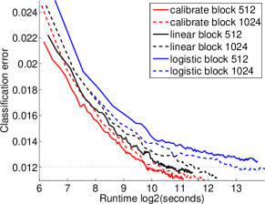
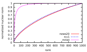
(a) Time vs Error	(b) Text vs Vision Data Spectrum

Figure 1: (a) Runtime versus error for different variants of our algorithms; (b) The fraction of the sum of the top 1000 singular values that is captured by the top $x$ singular values.

3.1 MNIST

Nonlinear classifiers are needed to achieve state-of-the-art performance in MNIST dataset. Although MNIST dataset only contains 60K data points (small by modern standards), the requirement for nonlinear features make this dataset computationally challenging. For instance, a nonlinear support vector machine with a Gaussian RBF kernel needs to manipulate a 60K$\times$60K kernel matrix. This will require hundreds of Gigabytes of memory, not available on most modern desktop machines. Hence we use an explicit feature representation and train our classifiers in the primal space. Specifically we construct random fourier features which are known to approximate the Gaussian kernel $k(x,x^{\prime})=\exp(-\|x-x^{\prime}\|^{2}/s)$ (Rahimi & Recht, 2007), though as discussed in the appendix various other methods to construct random low degree polynomials are also effective.

We start by comparing linear and logistic regression using Algorithm 1, as well as the calibration variant of Algorithm 2. For the calibration variant, we use a basis $G(y)$ consisting of $y$, $y^{2}$ and $y^{3}$ (applied elementwise to vector $y$). We compare these algorithms on raw pixel features, as well as small number of random Fourier features described above. As seen in Table 1, the performance of logistic and calibrated variants seem similar and consistently superior to plain linear regression.

Next, we move to improving accuracy by using the stagewise approach of Algorithm 3, which allows us to scale up to larger number of random Fourier features. Concretely, we fit blocks of features (either 512 and 1024) with Algorithm 3 with three alternative update rules on each stage: linear regression, calibrated linear regression, and logistic regression (with 50 inner loops for the logistic computations). Here, our calibrated linear regression is the simplest one: we only use the previous predictions as features in our new batch of features.

Our next experiment demonstrates that all three (extremely simple and parameter free) algorithms quickly achieve state of the art performance. Figure 1(a) shows the relation between feature block size, classification test error, and runtime for these algorithm variants. Importantly, while the linear (and linear calibration) algorithms do not achieve as low an error for a fixed feature size, they are faster to optimize and are more effective overall.

Table 1: Linear Regression vs. logistic regression vs. (polynomial) calibration. For the polynomial calibration, we refit our predictions with $\hat{y}$, $\hat{y}^{2}$ and $\hat{y}^{3}$.

Algorithm	Linear	Logistic	(poly.) Calibration
Raw pixels	14.1%	7.8%	8.1%
4000 dims	1.83 %	1.48 %	1.54 %
8000 dims	1.48%	1.33%	1.36%

Notably, we find that (i) linear regression achieves better runtime and error trade-off, even though for a fixed number of features linear regressions are not as effective as logistic regression (as we see in Figure 2(a)). (ii) relatively small size feature blocks provide better runtime and error trade-off (blocks of size 300 provide further improvements). (iii) the linearly calibrated regression works better than the vanilla linear regression.

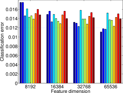
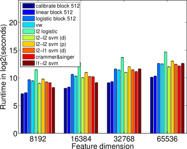
(a) Comparable Errors	(b) Time Comparisons

Figure 2: (a) Error comparison between our variants, VW and six variants of Liblinear: L2-regularized logistic regression, L2-regularized L2-loss support vector classification (dual), L2-regularized L2-loss support vector classification (primal), L2-regularized L1-loss support vector classification (dual), multi-class support vector classification by Crammer and Singer, L1-regularized L2-loss support vector classification. (b) Runtime comparison in log time.

We also compare these three variants of our approach to other state-of-the-art algorithms in terms of classification test error and runtime (Figure 2(a) and (b)). Note the logarithmic scaling of the runtime axes. The comparison includes VW , and six algorithms implemented in Liblinear (Fan et al., 2008) (see figure caption). We took care in our attempts to time these algorithms to reflect their actual computation time, rather than their loading of the features (which can be rather large, making it extremely time consuming to run these experiments); our stagewise algorithms generate new features on the fly so this is not an issue. See the appendix for further discussion.

From Figure 2 (a) and (b), our logistic algorithm is competitive with all the other algorithms, in terms of it’s accuracy (while for lower dimensions the naive linear methods fared a little worse). All of our algorithms were substantially faster.

Finally, the models produced by our methods drive the classification test error down to 1.1% while none of the competitors achieve this test error. Runtime wise, our method is extremely fast for the linear regression and calibrated linear regression variants, which are consistently at least 10 times faster than the other highly optimized algorithms. This is particularly notable given the simplicity of this approach.

3.2 CIFAR-10

The CIFAR-10 dataset is a more challenging dataset, where many image recognition algorithms have been tested (primarily illustrating different methods of feature generation; our work instead focusses on the optimization component, given a choice of features). The neural net approaches of “dropout” and “maxout” algorithms of (Hinton et al., 2012; Goodfellow et al., 2013) provide the best reported performance of 84% and 87%, without increasing the size of the dataset (through jitter or other transformations). We are able to robustly achieve over 85% accuracy with linear regression on standard convolution features (without increasing the size of the dataset through jitter, etc.), illustrating the advantage that improved optimization provides.

Figure 3 illustrates the performance when we use two types of convolutional features: features generated by convolving the images by random masks, and features generated by convolving with K-means masks (as in (Coates et al., 2011), though we do not use contrast normalization).

We find that using only relatively few filters (say about 400), along with polynomial features, are sufficient to obtain over $80\%$ accuracy extremely quickly. Hence, using the thousands of generated features, it is rather fast to build multiple models with disjoint features and model average them, obtaining extremely good performance.

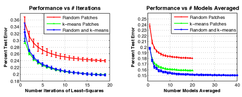
(a)                                                    (b)

Figure 3: CIFAR-10 results using two types of convolutional features: (a) features generated by convolving the images by random masks, and (b) features generated by convolving with K-means masks.

3.3 Well-Conditioned Problems

We now examine two popular multiclass text datasets: 20 newsgroups (henceforth NEWS20), which is a 20 class dataset and a four class version of Reuters Corpus Volume 1 (Lewis et al., 2004) (henceforth RCV1). We use a standard (log) term frequency representation of the data, discussed in the appendix. These data pose rather different challenges than our vision datasets; in addition to being sparse datasets, they are extremely well conditioned.

The ratio of the 2nd singular value to the 1000th one (as a proxy for the condition number) and is 19.8 for NEWS20 and 14 for RCV1. In contrast, for MNIST, this condition number is about 72000 (when computed with 3000 random Fourier features). Figure 1(b) shows the normalized spectrum for the three data matrices.

As expected, online first-order methods (in particular VW) fare far more favorably in this setting, as seen in Table 2. We use a particular greedy procedure for a our stagewise ordering (as discussed in the appendix, though random also works well). Note that this data is well suited for online methods: it is sparse (making the online updates cheap) and well conditioned (making the gap in convergence between online methods and second order methods small).

Ultimately, an interesting direction is developing hybrid approaches applicable to both cases.

Table 2: Running times and test errors in text datasets for VW, Liblinear, and Stagewise regression

	NEWS20		RCV1
Method	Time	%Error	Time	%Error
VW	2.5	12.4	2.5	2.75
Liblinear	27	13.8	120	2.73
Stagewise	40	11.7	240	2.77

4 Discussion

In this paper, we present a suite of fast and simple algorithms for tackling large-scale multiclass prediction problems. We stress that the key upshot of the methods developed in this work is their conceptual simplicity and ease of implementation. Indeed these properties make the methods quite versatile and easy to extend in various ways. We showed an instance of this in Algorithm 2. Similarly, it is straightforward to develop accelerated variants (Nesterov, 2009), by using the distances defined by the matrix $\widehat{\Sigma}$ as the prox-function in Nesterov’s work. These variants enjoy the usual improvements of $\mathcal{O}(1/t^{2})$ iteration complexity in the smooth and $\sqrt{\kappa_{\Phi}}$ dependence in the strongly convex setting, while retaining the metric-free nature of Algorithm 1.

It is also quite easy to extend the algorithm to multi-label settings, with the only difference being that the vector $y$ of labels now lives on the hypercube instead of the simplex. This only amounts to a minor modification of the projection step in Algorithm 2.

Overall, we believe that our approach revisits many old and deep ideas to develop algorithms that are practically very effective. We believe that it will be quite fruitful to understand these methods better both theoretically and empirically in further research.

Appendix A Appendix

A.1 Proofs

Proof of Theorem 1

We start by noting that the Lipschitz and strong monotonicity conditions on $\nabla\Phi$ imply the smoothness and strong convexity of the function $\Phi(u)$ as a function $u\in\mathbb{R}^{k}$. In particular, given any two matrices $W_{1},W_{2}\in\mathbb{R}^{k\times d}$, we have as the following quadratic upper bound as a consequence of the Lipschitz condition (16)

$$\Phi(W_{1}x)\leq\Phi(W_{2}x)+\left\langle\nabla\Phi(W_{2}x^{T})x,W_{1}-W_{2}\right\rangle+\frac{L}{2}\|W_{1}x-W_{2}x\|_{2}^{2}.$$

The strong monotonicity condition (17) yields an analogous lower bound

$$\Phi(W_{1}x)\geq\Phi(W_{2}x)+\left\langle\nabla\Phi(W_{2}x^{T})x,W_{1}-W_{2}\right\rangle+\frac{\mu}{2}\|W_{1}x-W_{2}x\|_{2}^{2}.$$

In order to proceed further, we need one additional piece of notation. Given a positive semi-definite matrix $M\in\mathbb{R}^{d\times d}$, let us define

$$\|W\|_{M}=\sum_{i=1}^{k}{W^{(i)}}^{T}MW^{(i)},$$

where $W^{(i)}$ is the $i$-th column of $W$, to be a Mahalanobis norm on matrices. Let us also recall the definition of the matrix $\widehat{\Sigma}$ from Algorithm 1. Then adding the smoothness condition over the examples $i=1,2,\ldots,n$ yields the following conditions on the sample average loss under condition (16):

$$\ell_{n}(W_{1})\leq\ell_{n}(W_{2})+\left\langle\nabla\ell_{n}(W_{2}),W_{1}-W_{2}\right\rangle+\frac{L}{2}\|W_{1}-W_{2}\|_{\widehat{\Sigma}}^{2}.$$

This implies that our objective function $\ell_{n}$ is $L$-smooth in the metric induced by $\widehat{\Sigma}$, and the update rule (14) corresponds to gradient descent on $\ell_{n}$ under this metric with a step-size of $1/L$. The first part of the theorem now follows from Corollary 2.1.2 of Nesterov (Nesterov, 2004).

As for the second part, we note that under the strong monotonicity condition, we have the lower bound

$$\ell_{n}(W_{1})\geq\ell_{n}(W_{2})+\left\langle\nabla\ell_{n}(W_{2}),W_{1}-W_{2}\right\rangle+\frac{\mu}{2}\|W_{1}-W_{2}\|_{\widehat{\Sigma}}^{2}.$$

Hence the objective $\ell_{n}$ is $\mu$-strongly convex and $L$-smooth in the metric induced by $\widehat{\Sigma}$. The result is now a consequence of Theorem 2.1.15 of Nesterov (Nesterov, 2004). ∎

We now provide the proof of Theorem 2. First, a little more on our assumption on $g^{-1}$. By convex duality, this inverse exists and if $\Phi$ is a closed, convex function then $(\nabla\Phi)^{-1}=\nabla\Phi^{*}$, where $\Phi^{*}$ is the Fenchel-Legendre conjugate of $\Phi$. Throughout this section, assume that $\nabla\Phi$ is $L$-Lipschitz continuous. By standard duality results regarding strong-convexity and smoothness, this implies that the conjugate $\Phi$ is $1/L$-strongly convex. Specifically, we have the useful inequality

$$\left\langle\nabla\Phi^{*}(u)-\nabla\Phi^{*}(v),u-v\right\rangle\geq\frac{1}{L}\|u-v\|_{2}^{2},\quad\mbox{for all}~{}~{}u,v\in\mathbb{R}^{k}.$$ (21)

Similarly, due to our assumption about the strong monotonicity of $\nabla\Phi$, it is the case that $\nabla\Phi^{*}$ is Lipschitz continuous and satisfies

$$\left\langle\nabla\Phi^{*}(u)-\nabla\Phi^{*}(v),u-v\right\rangle\leq\frac{1}{\mu}\|u-v\|_{2}^{2},\quad\mbox{for all}~{}~{}u,v\in\mathbb{R}^{k}.$$ (22)

As a specific consequence, note that it is natural to assume that $\nabla\Phi(0)=1\!\!1/k$, where $1\!\!1$ is the all ones vector. That is the expectation is uniform over all the labels when the weights are zero. Under this condition, it is easy to obtain as a consequence of Equation 22 that

$$\|\nabla\Phi^{*}(u)\|_{2} =\|\nabla\Phi^{*}(u)-\nabla\Phi^{*}(1\!\!1/k)\|_{2}$$

$$\leq\frac{1}{\mu}\|u-1\!\!1/k\|_{2}\leq\frac{1}{\mu}\left(\|u\|_{2}+\frac{1}{\sqrt{k}}\right).$$ (23)

Together with these facts, we now proceed to establish Theorem 2.

Proof of Theorem 2

We will use $\bar{y}^{{t}}_{i}=\tilde{W}_{t}G(\tilde{y}^{(t)}_{i})$ to denote the predictions at each iteration before the clipping operation. For brevity, we use $\hat{Y}^{(t)}\in\mathbb{R}^{n\times k}$ to denote the matrix of all the predictions at iteration $t$, with a similar version $\tilde{Y}^{{t}}$ for $\tilde{y}^{(t)}$

The following basic properties of linear regression that are helpful. By the optimality conditions for $W_{i}$ and $\tilde{W}_{i}$,

$$\sum_{i=1}^{n}(\tilde{y}^{(t)}_{i}-y_{i})x_{i}^{T} =\mathbf{0}_{k\times d},\quad\mbox{and}$$

$$\sum_{i=1}^{n}(\bar{y}^{{t}}_{i}-y_{i})G(\tilde{y}^{(t-1)}_{i})^{T} =\mathbf{0}_{|G|\times d}.$$ (24)

In particular, multiplying the first equality with the optimal weight matrix $W^{*}$ yields

$$\left\langle\sum_{i=1}^{n}(\tilde{y}^{(t)}_{i}-y_{i})x_{i}^{T},W^{*}\right\rangle=0.$$

Rearranging terms and recalling that $\nabla\Phi(W^{*}x_{i})=y_{i}$ due to the generative model (12) further allows us to rewrite

$$\left\langle\sum_{i=1}^{n}(\tilde{y}^{(t)}_{i}-y_{i}),\nabla\Phi^{*}(y_{i})\right\rangle=0.$$ (25)

Combining this with our earlier inequality (21) further yields

$$\sum_{i=1}^{n}\left\langle\tilde{y}^{(t)}_{i}-y_{i},\nabla\Phi^{*}(\tilde{y}^{(t)}_{i})\right\rangle =\sum_{i=1}^{n}\left\langle\tilde{y}^{(t)}_{i}-y_{i},\nabla\Phi^{*}(\tilde{y}^{(t)}_{i})-\nabla\Phi^{*}(y_{i})\right\rangle\geq\frac{1}{L}\sum_{i=1}^{n}\|\tilde{y}^{(t)}_{i}-y_{i}\|_{2}^{2}.$$ (26)

Having lower bounded this inner product term, we obtain an upper bound on it which will complete the proof for convergence of the algorithm. Note that $\tilde{W}_{t}$ minimizes the objective (19). Since $\nabla\Phi^{*}\in\mbox{lin}(G)$, we have for any constant $\beta\in\mathbb{R}$

$$\sum_{i=1}^{n}\|\bar{y}^{{t}}_{i}-y_{i}\|_{2}^{2}\leq\sum_{i=1}^{n}\|\tilde{y}^{(t)}_{i}-y_{i}-\beta\nabla\Phi^{*}(\tilde{y}^{(t)})\|_{2}^{2}.$$

We optimize over the choices of $\beta$ to obtain the best inequality above, which yields the error reduction as

$$\sum_{i=1}^{n}\|\bar{y}^{{t}}_{i}-y_{i}\|_{2}^{2} \leq\sum_{i=1}^{n}\|\tilde{y}^{(t)}_{i}-y_{i}\|_{2}^{2}-\frac{\left\langle\tilde{Y}^{{t}}-Y,\nabla\Phi^{*}(\tilde{Y}^{{t}})\right\rangle^{2}}{\|\nabla\Phi^{*}(\tilde{Y}^{{t}})\|_{F}^{2}}.$$ (27)

We now proceed to upper bound the denominator in the second term in the right hand side of the above bound. Note that from Equation 23, we have the upper bound

$$\|\nabla\Phi^{*}(\tilde{y}^{(t)}_{i})\|_{2}^{2} \leq\frac{2}{\mu^{2}}\left(\|\hat{y}^{(t)}_{i}\|_{2}^{2}+\frac{1}{k}\right)$$

$$\leq\frac{2}{\mu^{2}k}+\frac{4}{\mu^{2}}\left(\|\tilde{y}^{(t)}_{i}-y_{i}\|_{2}^{2}+\|y_{i}\|_{2}^{2}\right)$$

$$\leq\frac{2}{\mu^{2}k}+\frac{4}{\mu^{2}}\left(\|\tilde{y}^{(t)}_{i}-y_{i}\|_{2}^{2}+1\right),$$

where the final inequality follows since $y_{i}$ has a one in precisely one place and zeros elsewhere. Adding these inequalities over the examples, we further obtain

$$\sum_{i=1}^{n}\|\nabla\Phi^{*}(\tilde{y}^{(t)}_{i})\|_{2}^{2} \leq\frac{2n}{\mu^{2}k}+\frac{4}{\mu^{2}}\left(\sum_{i=1}^{n}\|\tilde{y}^{(t)}_{i}-y_{i}\|_{2}^{2}+n\right)$$

$$\leq\frac{6n}{\mu^{2}}+\frac{4}{\mu^{2}}\sum_{i=1}^{n}\|\hat{y}^{(t)}_{i}-y_{i}\|_{2}^{2},$$

where the last step is an outcome of solving the regression problem in the step (18). Finally, observe that $\hat{y}^{(t)}$ is a probability vector in $\mathbb{R}^{k}$ as a result of the clipping operation, while $y_{i}$ is a basis vector as before. Taking these into account, we obtain the upper bound

$$\sum_{i=1}^{n}\|\nabla\Phi^{*}(\tilde{y}^{(t)}_{i})\|_{2}^{2}\leq\frac{22nk}{\mu^{2}}.$$ (28)

We are almost there now. Observe that we can substitute this upper bound into our earlier inequality (27) and obtain

$$\sum_{i=1}^{n}\|\bar{y}^{{t}}_{i}-y_{i}\|_{2}^{2} \leq\sum_{i=1}^{n}\|\tilde{y}^{(t)}_{i}-y_{i}\|_{2}^{2}-\frac{\mu^{2}}{22nk}\left\langle\tilde{Y}^{{t}}-Y,\nabla\Phi^{*}(\tilde{Y}^{{t}})\right\rangle^{2}.$$ (29)

We can further combine this inequality with the lower bound (26) and obtain

$$\sum_{i=1}^{n}\|\bar{y}^{{t}}_{i}-y_{i}\|_{2}^{2} \leq\sum_{i=1}^{n}\|\tilde{y}^{(t)}_{i}-y_{i}\|_{2}^{2}-\frac{\mu^{2}}{22nkL^{2}}\left(\sum_{i=1}^{n}\|\tilde{y}^{(t)}_{i}-y_{i}\|_{2}^{2}\right)^{2}.$$ (30)

This would yield a recursion if we could replace the term $\sum_{i=1}^{n}\|\bar{y}^{{t}}_{i}-y_{i}\|_{2}^{2}$ with $\sum_{i=1}^{n}\|\tilde{y}^{(t+1)}_{i}-y_{i}\|_{2}^{2}$. This requires the use of two critical facts. Note that $\hat{y}^{(t)}_{i}$ is a Euclidean projection of $\bar{y}^{{t}}_{i}$ onto the probability simplex and $y_{i}$ is an element of the simplex. Consequently, by Pythagoras theorem, it is easy to conclude that

$$\|\hat{y}^{(t)}_{i}-y_{i}\|^{2}\leq\|\bar{y}^{{t}}_{i}-y_{i}\|_{2}^{2}.$$

Furthermore, the regression update (18) guarantees that we have

$$\sum_{i=1}^{n}\|\tilde{y}^{(t+1)}-y_{i}\|_{2}^{2}\leq\sum_{i=1}^{n}\|\hat{y}^{(t)}_{i}-y_{i}\|_{2}^{2}\leq\sum_{i=1}^{n}\|\bar{y}^{{t}}_{i}-y_{i}\|_{2}^{2}.$$

Combining the update with earlier bound (30), we finally obtain the recursion we were after:

$$\sum_{i=1}^{n}\|\tilde{y}^{(t+1)}_{i}-y_{i}\|_{2}^{2} \leq\sum_{i=1}^{n}\|\tilde{y}^{(t)}_{i}-y_{i}\|_{2}^{2}-\frac{\mu^{2}}{22nkL^{2}}\left(\sum_{i=1}^{n}\|\tilde{y}^{(t)}_{i}-y_{i}\|_{2}^{2}\right)^{2}.$$ (31)

Let us define $\epsilon_{t}=\frac{1}{n}\sum_{i=1}^{n}\|\tilde{y}^{(t)}_{i}-y_{i}\|_{2}^{2}$. Then the above recursion can be simplified as

$$\epsilon_{t+1} \leq\epsilon_{t}-\frac{\mu^{2}}{22n^{2}kL^{2}}\left(\sum_{i=1}^{n}\|\tilde{y}^{(t)}_{i}-y_{i}\|_{2}^{2}\right)^{2}$$

$$=\epsilon_{t}-\frac{\mu^{2}}{22kL^{2}}\epsilon_{t}^{2}.$$

It is straightforward to verify that the recursion is satisfied by setting $\epsilon_{t}=22kL^{2}/(\mu^{2}t)=22\kappa_{\Phi}^{2}/t$. Lastly, observe that as a consequence of the update (19) and the contractivity of the projection operator, we also have

$$\frac{1}{n}\sum_{i=1}^{n}\|\hat{y}^{(t)}_{i}-y_{i}\|_{2}^{2}\leq\frac{1}{n}\sum_{i=1}^{n}\|\tilde{y}^{(t)}_{i}-y_{i}\|_{2}^{2}\leq\frac{22\kappa_{\Phi}^{2}}{t},$$

which completes our proof.

∎

A.2 Experimental Details

A.2.1 MNIST

We utilize random Fourier features after PCA-ing the data down to $50$ dimensions. This projection alone is a considerable speed improvement (for all algorithms) with essentially no loss in accuracy. We then applied the random features as described in (Rahimi & Recht, 2007). We should note that our reliance on these features is not critical; both random low degree polynomials or random logits (with weights chosen from Gaussian distribution of appropriate variance, so the features have reasonable sensitivity) give comparable performance. Notably, the random logits seem to need substantially fewer features to get to the same accuracy level (maybe by a factor of 2).

The kernel bandwidth $s$ is set using the folklore “median trick”, i.e., $s$ is the median pairwise distance between training points.

For VW, we first generated its native binary input format. VW uses a separate thread for loading data, so that the data loading time is negligible. For Liblinear, we used a modified version which can directly accept dense input features from MATLAB. As with the rest of the experiments, our methods are implemented in MATLAB. For all methods, the computation for model fitting is done in a single 2.4 GHz processor.

A.2.2 20 Newsgroups and RCV1

Our theoretical understanding suggests that when the condition number is small then we expect first order methods to be highly effective. Furthermore, these methods enjoy an extra computational advantage when the data is sparse, as the computation of the gradient updates are linear time in the sparsity level. Here, as expected, methods that ignore second order information are faster than stagewise procedures.

We used unigram features with with $\log$-transformed term frequencies as values. We also removed all words that appear fewer than 3 times on the training set. For RCV1 the task was to predict whether a news story should be classified as “corporate”, “economics”, “government”, or “markets”. Stories belonging to more than one category were removed. For RCV1, we switched the roles of training and test folds with 665 thousand and 20 thousand examples for training and testing respectively. Tokens in RCV1 had already been stemmed and stopwords had been removed resulting in about 20000 features. For NEWS20 we did not perform such preprocessing leading to about 44000 features. We split the data into 15000 for training and the rest for testing.

For both datasets the bag of words representation is too “verbose” to handle efficiently with commodity hardware. Therefore, we exclusively used the stagewise approach here. In each stage, we picked a subset of the original features (i.e., no random projections). To speed up the algorithm, we ordered the features by the magnitude of the gradient.

For NEWS20 we used a batch size of 500, 2 passes over the data and regularization $\lambda=30$. We recomputed the ordering between the first and second pass. For RCV1 we used 2 batches of size 2000 and computed the ordering for each batch. The results are shown in Table 2(b). Even though the stagewise procedure can produce models with the same or better generalization error than Liblinear and VW, it is not as efficient. This is again no surprise since when the condition number is small, methods based on stochastic gradient, such as VW, are optimal (Bottou & Bousquet, 2008).

References

- Agarwal (2013) Agarwal, A. Selective sampling algorithms for cost-sensitive multiclass prediction. In ICML, 2013.
- Bordes et al. (2009) Bordes, A., Bottou, L., and Gallinari, P. Sgd-qn: Careful quasi-newton stochastic gradient descent. Journal of Machine Learning Research, 10:1737–1754, July 2009.
- Bottou & Bousquet (2008) Bottou, L. and Bousquet, O. The tradeoffs of large scale learning. In NIPS. 2008.
- Bronshtein (1976) Bronshtein, E.M. -entropy of convex sets and functions. Siberian Mathematical Journal, 17(3):393–398, 1976.
- Byrd et al. (2011) Byrd, R. H., Chin, G. M., Neveitt, W., and Nocedal, J. On the use of stochastic hessian information in optimization methods for machine learning. SIAM Journal on Optimization, 21(3):977–995, 2011.
- Chapelle (2007) Chapelle, O. Training a support vector machine in the primal. Neural Comput., 19(5):1155–1178, 2007.
- Coates et al. (2011) Coates, A., Ng, A. Y., and Lee, H. An analysis of single-layer networks in unsupervised feature learning. Journal of Machine Learning Research - Proceedings Track, 15:215–223, 2011.
- Collins & Koo (2000) Collins, M. and Koo, T. Discriminative reranking for natural language parsing. In ICML, 2000.
- Duchi et al. (2008) Duchi, J., Shalev-Shwartz, S., Singer, Y., and Chandra, T. Efficient projections onto the -ball for learning in high dimensions. In ICML, 2008.
- Fan et al. (2008) Fan, R.-E., Chang, K.-W., Hsieh, C.-J., Wang, X.-R., and Lin, C.-J. Liblinear: A library for large linear classification. Journal of Machine Learning Research, 9:1871–1874, 2008.
- Friedman (2001) Friedman, J. H. Greedy function approximation: a gradient boosting machine.(english summary). Ann. Statist, 29(5):1189–1232, 2001.
- Goodfellow et al. (2013) Goodfellow, I. J., Warde-Farley, D., Mirza, M., Courville, A. C., and Bengio, Y. Maxout networks. CoRR, 2013.
- Hinton et al. (2012) Hinton, G. E., Srivastava, N., Krizhevsky, A., Sutskever, I., and Salakhutdinov, R. R. Improving neural networks by preventing co-adaptation of feature detectors. arXiv preprint arXiv:1207.0580, 2012.
- Jebara & Choromanska (2012) Jebara, T. and Choromanska, A. Majorization for crfs and latent likelihoods. In NIPS, 2012.
- Kakade et al. (2011) Kakade, S. M., Kalai, A., Kanade, V., and Shamir, O. Efficient learning of generalized linear and single index models with isotonic regression. In NIPS, 2011.
- Kalai & Sastry (2009) Kalai, A. T. and Sastry, R. The isotron algorithm: High-dimensional isotonic regression. In COLT ’09, 2009.
- Lauritzen (1996) Lauritzen, S. L. Graphical Models. Oxford University Press, Oxford, 1996.
- Lewis et al. (2004) Lewis, D. D., Yang, Y., Rose, T. G., and Li, F. Rcv1: A new benchmark collection for text categorization research. The Journal of Machine Learning Research, 5:361–397, 2004.
- Matsushima et al. (2012) Matsushima, S., Vishwanathan, S. V. N., and Smola, A. J. Linear support vector machines via dual cached loops. In KDD, 2012.
- Nemirovsky & Yudin (1983) Nemirovsky, A. S. and Yudin, D. B. Problem Complexity and Method Efficiency in Optimization. New York, 1983.
- Nesterov (2004) Nesterov, Y. Introductory Lectures on Convex Optimization. New York, 2004.
- Nesterov (2009) Nesterov, Y. Primal-dual subgradient methods for convex problems. Mathematical Programming A, 120(1):261–283, 2009.
- Nesterov (2012) Nesterov, Y. Efficiency of coordinate descent methods on huge-scale optimization problems. SIAM Journal on Optimization, 22(2):341–362, 2012.
- Platt (1999) Platt, J. C. Probabilistic outputs for support vector machines and comparisons to regularized likelihood methods. In Adavances in large margin classifiers, pp. 61–74. MIT Press, 1999.
- Rahimi & Recht (2007) Rahimi, A. and Recht, B. Random features for large-scale kernel machines. Advances in neural information processing systems, 20:1177–1184, 2007.
- Ravikumar et al. (2008) Ravikumar, P., Wainwright, M., and Yu, B. Single index convex experts: Efficient estimation via adapted bregman losses. Snowbird learning workshop, 2008. URL http://snowbird.djvuzone.org/2008/abstracts/183.pdf.
- Recht et al. (2011) Recht, B., Re, C., Wright, S. J., and Niu, F. Hogwild: A lock-free approach to parallelizing stochastic gradient descent. In NIPS, pp. 693–701, 2011.
- Richtárik & Takác (2012) Richtárik, P. and Takác, M. Parallel coordinate descent methods for big data optimization. 2012. URL http://arxiv.org/abs/1212.0873.
- Rockafellar (1966) Rockafellar, R.T. Characterization of the subdifferentials of convex functions. Pac. J. Math., 17:497–510, 1966.
- Roux et al. (2012) Roux, N. L., Schmidt, M., and Bach, F. A stochastic gradient method with an exponential convergence rate for finite training sets. In NIPS, pp. 2672–2680. 2012.
- Shalev-Shwartz (2012) Shalev-Shwartz, S. Online learning and online convex optimization. Foundations and Trends in Machine Learning, 4(2), 2012.
- Shalev-Shwartz & Zhang (2013) Shalev-Shwartz, S. and Zhang, T. Stochastic Dual Coordinate Ascent Methods for Regularized Loss Minimization. Journal of Machine Learning Reearch, 14:567–599, 2013.
- Yu et al. (2012) Yu, H.-F., Hsieh, C.-J., Chang, K.-W., and Lin, C.-J. Large linear classification when data cannot fit in memory. TKDD, 5(4), 2012.