QUANTUM SPINDOWN OF HIGHLY MAGNETIZED NEUTRON STARS

Pulsars are highly magnetized and rapidly rotating neutron stars. The magnetic field can reach the critical magnetic field from which quantum effects of the vacuum becomes relevant, giving rise to magnetooptic properties of vacuum characterized as an effective non linear medium. One spectacular consequence of this prediction is a macroscopic friction that leads to an additionnal contribution in the spindown of pulsars. In this paper, we highlight some observational consequences and in particular derive new constraints on the parameters of the Crab pulsar and J0540-6919.

1 Introduction

It is known from long time that quantum effects give to vacuum its own electromagnetic properties, in analogy with a usual ponderable media (for a recent review, see for example $\!{}^{{\bf?}}$). Among experimentally accessible consequences are photon/photon scattering $\!{}^{{\bf?}}$ or vacuum birefringence $\!{}^{{\bf?}}$, both being targeted by laboratory experiments. Astrophyscial objects such as Neutron Stars (NS) are also a laboratory to test those quantum corrections, simply because they sustain a very high magnetic field that enhances the quantum features of vacuum. In particular, when the magnetic energy around a NS is comparable to the electron rest energy, $B\sim B_{c}=\frac{m_{e}^{2}c^{2}}{e\hbar}$, a significant magnetization arise in the vacuum that give rise to spectacular macroscopic consequences on the spindown of this NS $\!{}^{{\bf?},{\bf?}}$.

The physical principle of the quantum contribution to the spindown is rather simple. The extremely high magnetic field, generated by the rotating dipole $\bm{m}$, creates a time-dependent magnetization in the vacuum around the NS. In return, this magnetization creates a magnetic field $\bm{B}_{\mathrm{qu}}$ which feeds back on the NS magnetic dipole. Due to retardation effect (finite speed of light), this back-action leads to a torque $\bm{m}\times\bm{B}_{\mathrm{qu}}$ that slows down the spinning of the NS. It has been shown that the energy loss rate of an isolated pulsar via the previous quantum channel, in the limit $B_{0}\ll B_{c}$, is given by $\!{}^{{\bf?},{\bf?}}$

$$\dot{E}_{\mathrm{qu}}=-\alpha\left(\frac{3\pi^{2}}{4}\right)\frac{\sin^{2}{\theta}}{B_{c}^{2}\mu_{0}c}\frac{B_{0}^{4}R^{4}}{P^{2}}\;,$$ (1)

where $\alpha$ is the fine structure constant, $\theta$ the inclination angle, $B_{0}$ the surface magnetic field, $c$ the speed of light, $R$ the radius of the NS and $P=2\pi/\Omega$ the rotation period. This contribution is an additional one compared to the classical spindown, which scales differently with respect to the physical parameters of the NS. Within the vacuum model (oblique rotator in vacuum), the energy loss rate is given by the usual dipole formula

$$\dot{E}_{\mathrm{cl}}=-\frac{128\pi^{5}}{3}\frac{B_{0}^{2}\sin^{2}\theta R^{6}}{P^{4}\mu_{0}c^{3}}\;,$$ (2)

where we can see that the classical contribution scales as $P^{-4}$ instead of the $P^{-2}$ for the quantum one. Both contributions are roughly of the same order when $\frac{B_{0}}{B_{c}}\sim\frac{R\Omega}{c}\frac{1}{\sqrt{\alpha}}\frac{1}{\sin\theta}$. Therefore, even if the magnetic field is much smaller than the critical magnetic field, the quantum contribution will dominate the classical one for large period P (or low $\Omega$). Hence, the late-time evolution of the spindown of a pulsar should generically be quantum-dominated, because the period gradually increases as the NS loses energy. Of course, this conclusion holds only in the simple model considered here, which is certainly incomplete. Among the physical phenomena that could change the previous statement are for instance the inclusion of a real magnetosphere, or taking into account an alignment of the NS (ie $\sin\theta\rightarrow 0$ as times passes $\!{}^{{\bf?}}$).

2 Quantum spindown

Using equations (1)-(2) and assuming the total energy is only rotational kinetic energy $E=\frac{1}{2}J\Omega^{2}$ ($J$ being the inertia moment), one gets a new evolution equation for the rotation period,

$$\dot{E}=\dot{E}_{\mathrm{cl}}+\dot{E}_{\mathrm{qu}}\quad\Rightarrow\quad\dot{P}=\frac{\mathcal{T}_{\mathrm{cl}}}{P}+\frac{P}{\mathcal{T}_{\mathrm{qu}}}\>,$$ (3)

where the constants $\mathcal{T}_{\mathrm{cl}}$ and $\mathcal{T}_{\mathrm{qu}}$ are easily obtained,

$$\mathcal{T}_{\mathrm{cl}} \simeq 8.8\times 10^{-16}\,\text{s}\left(\frac{B_{0}}{10^{8}\,\text{T}}\right)^{2}\sin^{2}\theta\left(\frac{R}{10\,\text{km}}\right)^{4}\left(\frac{1.4\,\text{M}_{\odot}}{M}\right)\;;$$ (4)

$$\mathcal{T}_{\mathrm{qu}} \simeq 2.1\times 10^{13}\,\text{s}\,\left(\frac{10^{8}\,\text{T}}{B_{0}}\right)^{4}\frac{1}{\sin^{2}\theta}\left(\frac{10\,\text{km}}{R}\right)^{2}\left(\frac{M}{1.4\,\text{M}_{\odot}}\right)\;.$$ (5)

It is clear that the quantum contribution will be dominant once $P>\mathcal{T}\equiv\sqrt{\mathcal{T}_{\mathrm{cl}}\mathcal{T}_{\mathrm{qu}}}$, with $\mathcal{T}\simeq 140\,\text{ms}\left(\frac{10^{8}\,\text{T}}{B_{0}}\right)\left(\frac{R}{10\,\text{km}}\right)$ a characteristic time. From the measurement of $P_{0}$, $P_{1}$ and $n_{0}$, respectively the present period, its first derivative and the braking index ($n\equiv 2-P\ddot{P}/\dot{P}^{2}$), it is possible to solve equation (3) and determine $\mathcal{T}_{\mathrm{cl}}$ and $\mathcal{T}_{\mathrm{qu}}$,

$$P(t)=\mathcal{T}\left[\left(1+\frac{P_{0}^{2}}{\mathcal{T}^{2}}\right)e^{\frac{t}{\mathcal{T}_{\mathrm{qu}}}}-1\right]^{1/2}\quad,\quad\mathcal{T}_{\mathrm{cl}}=P_{0}P_{1}\frac{n_{0}-1}{2}\quad,\quad\mathcal{T}_{\mathrm{qu}}=\frac{P_{0}}{P_{1}}\frac{2}{3-n_{0}}\;.$$ (6)

As an explicit example, the evolution of the Crab pulsar from the previous expressions is represented in the $(P,\dot{P})$ diagramm of figure 1. The evolution starts from the birth of the Crab ($\leavevmode\nobreak\ 955$ years ago) and last $50\,$kyr. Each dot in this plot is a pulsar from the ATNF catalog $\!{}^{{\bf?}}$. The interesting feature is that the evolution naturally brings the Crab towards the so-called magnetar region in the upper right corner, even if the magnetic field is smaller than the critical field (see next section for an estimation of the Crab magnetic field, being a few $10^{8}\,$T). This could support the idea already proposed in $\!{}^{{\bf?}}$ that some of the so-called magnetars are in fact normal evolved pulsars. A deeper analysis of this hypothesis is underway.

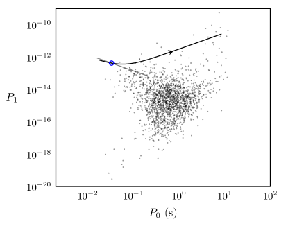
Figure 1: Evolution of the Crab pulsar. The grey line is the classical evolution while the black line is the evolution taking into account the quantum correction.

The quantum evolution given by (6) also has a consequence on the age of the pulsar, obtained as

$$t_{\text{age}}=\frac{P_{0}}{P_{1}}\frac{1}{n_{0}-3}\,\ln\frac{n_{0}-1+(3-n_{0})\frac{P_{i}^{2}}{P_{0}^{2}}}{2}\mathrel{\mathop{\sim}\limits_{P_{i}\ll P_{0}}}\frac{P_{0}}{(3-n_{0})P_{1}}\ln\frac{n_{0}-1}{2}$$ (7)

The last equality assumes that the present period $P_{0}$ is much greater than the initial period $P_{i}$. This age is always greater than the characteristic age $\frac{P_{0}}{2P_{1}}$ obtained classically with the same approximation $P_{i}\ll P_{0}$. This consequence could be an observational signature of the quantum evolution since it would show up as a systematic bias between the kinematical age (or SNR age) and the characteristic age. Such discrepancies are for example reported in $\!{}^{{\bf?}}$.

3 Constraints on the mass and radius

From $\mathcal{T}_{\mathrm{cl}}$ and $\mathcal{T}_{\mathrm{qu}}$, it is straightforward to determine $B_{0}$ and $\sin\theta$ as a function of the mass $M$ and the radius $R$ of the NS, giving

$$B_{0} = \frac{5\pi B_{c}R}{2c\sqrt{\alpha}}\frac{1}{P_{0}}\sqrt{\frac{3-n_{0}}{n_{0}-1}}\;;$$ (8)

$$\sin^{2}\theta = \frac{3\alpha}{400\pi^{5}}\frac{\mu_{0}Jc^{5}}{R^{8}B_{c}^{2}}P_{0}^{3}P_{1}\frac{(n_{0}-1)^{2}}{3-n_{0}}\;.$$ (9)

The condition $\sin^{2}\theta<1$ then provides constraints on the mass $M$ and the radius $R$ of the pulsar. Such constraints are represented in the figure 2 as exclusion regions, for two similar pulsars, namely $J0534+2200$ (the Crab) and $J0540-6919$; for those pulsars the braking index $n_{0}$ is confidently measured and is given in table 1. For sake of simplicity we assumed $J=\frac{2}{5}MR^{2}$. In the same figure are represented some families of Equation Of State for the NS (extracted from $\!{}^{{\bf?}}$). It is quite remarkable that taking into account the quantum effect sets some constraints on such EOS. In particular, the strange quark models (SQM) seem excluded. Of course, it is not possible to draw any definite conclusion unless a more realistic model is studied. For example, it is expected that the magnetosphere could significantly change the previous conclusions.

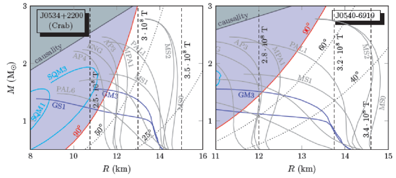
Figure 2: Constraints in the $(M,R)$ diagramm. The colored regions are excluded, either by causality or by the condition $\sin\theta<1$. The solid lines corresponds to different models of NS equation of state. The dotted lines correspond to constant value of the inclination angle while vertical dashed lines correspond to constant magnetic field $B_{0}$.

Table 1: Spin and breaking index.

Name	$n_{0}$	$P_{0}$	$P_{1}$
J2000		(ms)	($10^{-13}$)
J0534+2200 (Crab)	2.51	33.1	4.23
J0540-6919	2.14	50.5	4.79

4 Conclusion

We showed that the predicted quantum-induced spindown in NS leads to observational consequences that should be looked for carefully. In particular, the evolution of a pulsar in the $(P,\dot{P})$ diagramm is qualitatively changed for highly manetized pulsars, the true age of a pulsar significantly differs from the characteristic age, and some constraints on the equation of state can be obtained, through new relationships between the mass, the radius, the inclination angle and the magnetic field of the NS.

References

References

- [1] R Battesti and C Rizzo. Magnetic and electric properties of a quantum vacuum. Reports on Progress in Physics, 76(1):6401, January 2013.
- [2] David d’Enterria and Gustavo G Silveira. Observing light-by-light scattering at the Large Hadron Collider. arXiv.org, page 7142, May 2013.
- [3] P Berceau, M Fouché, R Battesti, and C Rizzo. Magnetic linear birefringence measurements using pulsed fields. Physical Review A, 85(1):13837, January 2012.
- [4] A Dupays, C Rizzo, D Bakalov, and G F Bignami. Quantum Vacuum Friction in highly magnetized neutron stars. EPL (Europhysics Letters), 82(6):69002, June 2008.
- [5] Arnaud Dupays, Carlo Rizzo, and Giovanni Fabrizio Bignami. Quantum vacuum influence on pulsars spindown evolution. Europhysics Letters, 98(4):49001, May 2012.
- [6] M D T Young, L S Chan, R R Burman, and D G Blair. Pulsar magnetic alignment and the pulsewidth-age relation. Monthly Notices of the Royal Astronomical Society, 402(2):1317–1329, February 2010.
- [7] R N Manchester, G B Hobbs, A Teoh, and M Hobbs. The Australia Telescope National Facility Pulsar Catalogue. The Astronomical Journal, 129(4):1993–2006, April 2005.
- [8] M A McLaughlin, Z Arzoumanian, J M Cordes, D C Backer, A N Lommen, D R Lorimer, and A F Zepka. PSR J1740+ 1000: A young pulsar well out of the Galactic plane. Astrophysical Journal, 564(1):333, 2002.
- [9] James M Lattimer. Equation of state constraints from neutron stars. Astrophysics and Space Science, 308(1):371–379, April 2007.