Bayes-X: a Bayesian inference tool for the analysis of X-ray observations of galaxy clusters

Abstract

We present the first public release of our Bayesian inference tool, Bayes-X, for the analysis of X-ray observations of galaxy clusters. We illustrate the use of Bayes-X by analysing a set of four simulated clusters at $z=0.2-0.9$ as they would be observed by a Chandra-like X-ray observatory. In both the simulations and the analysis pipeline we assume that the dark matter density follows a spherically-symmetric Navarro, Frenk and White (NFW) profile and that the gas pressure is described by a generalised NFW (GNFW) profile. We then perform four sets of analyses. These include prior-only analyses and analyses in which we adopt wide uniform prior probability distributions on $f_{\rm g}(r_{200})$ and on the model parameters describing the shape and slopes of the GNFW pressure profile, namely $(c_{500},a,b,c)$. By numerically exploring the joint probability distribution of the cluster parameters given simulated Chandra-like data, we show that the model and analysis technique can robustly return the simulated cluster input quantities, constrain the cluster physical parameters and reveal the degeneracies among the model parameters and cluster physical parameters. We then use Bayes-X to analyse Chandra data on the nearby cluster, A262, and derive the cluster physical and thermodynamic profiles. The results are in good agreement with other results given in literature for the cluster. To illustrate the performance of the Bayesian model selection, we also carried out analyses assuming an Einasto profile for the matter density and calculated the Bayes factor. The results of the model selection analyses for the simulated data favour the NFW model as expected. However, we find that the Einasto profile is preferred in the analysis of A262. The Bayes-X software, which is implemented in Fortran 90, is available at http://www.mrao.cam.ac.uk/facilities/software/bayesx/.

1 Introduction

Clusters of galaxies, as the most massive gravitationally bound material structures, are of basic importance in the study of both baryonic and dark-matter density distributions in the Universe. In practice, measurement of line-of-sight velocity dispersions of the galaxies in a cluster (see e.g. Rines, Geller & Diaferio 2010 and Sifón et al. 2013), observation of X-ray emission from the hot gas in a cluster’s gravitational potential well (see e.g. Vikhlinin et al. 2005, 2006; Allen, Evrard & Mantz 2011; Russell et al. 2012 and Sanders & Fabian 2013), observation at microwave frequencies of the SZ (Sunyaev & Zeldovich, 1970) effect (see e.g. AMI Consortium: Shimwell et al. 2013 and Planck Collaboration et al. 2013) and measurement of the gravitational lensing of background galaxies by the cluster potential (see e.g. Corless, King & Clowe 2009 and AMI Consortium: Hurley-Walker et al. 2012) are all key in assessing the matter distribution in clusters. However, each method has different strengths and weaknesses. Historically, the majority of the studies on the measurement of galaxy cluster masses have been in the X-ray band, and we consider X-ray measurement and analysis in this paper.

The motivation for our work is to augment the high resolution X-ray observations of clusters with an analysis pipeline that comprises (a) a cluster model consistent with both numerical simulations and real observations of clusters, and (b) a Bayesian statistical method. This provides an interesting and very powerful way to investigate the constraints on the cluster physical parameters imposed by X-ray data.

The great majority of X-ray (and indeed of SZ) measurements of cluster masses in the literature assume parameterised functional forms for the radial distribution of two independent cluster thermodynamic properties, such as electron density and temperature, to model the X-ray surface brightness (see e.g. Sarazin 1988; Vikhlinin et al. 2005, 2006; LaRoque et al. 2006; AMI Consortium: Olamaie et al. 2012 and Planck Collaboration et al. 2013). These radial profiles (e.g. $\beta$-model) have an amplitude normalisation parameter and two or more shape parameters.

In Bayes-X we use our recently developed cluster model (Olamaie et al., 2012, 2013) to parameterise the radial X-ray surface brightness profile and explore the constraints on both model parameters and physical parameters of simulated Chandra- like observations of four clusters. The model, hereafter model (I), assumes that the dark matter density follows a Navarro, Frenk and White (NFW) profile (Navarro, Frenk & White, 1996, 1997) and the ICM plasma pressure is described by the generalised NFW (GNFW) profile (Nagai, Kravtsov & Vikhlinin, 2007; Arnaud et al., 2010), both in accordance with numerical simulations that take into account radiative cooling, star formation and energy feedback from supernova explosions (see e.g. Borgani 2004; Nagai, Kravtsov & Vikhlinin 2007 and Piffaretti & Valdarnini 2008).

Computational advances allow us to compare the model with the data in a fully Bayesian fashion (see e.g. Jaynes 1986 and Sivia 2005), which has the well-known advantages of employing prior information and in dealing with probability distributions of any shape rather than just a mean value and an error-bar. This is linked to ability of the method to explore degeneracies that would otherwise be hidden. The importance of this property will become clear in this paper.

A Bayesian approach has been previously used in the X-ray analysis of galaxies and galaxy clusters (see e.g. Mahdavi et al. 2007, Humphrey et al. 2009, Humphrey et al. 2011 and Humphrey et al. 2012). In all of these studies, the spectra are extracted in concentric annuli around the cluster centre requiring annular widths to be large enough to give significant counts. The data also need to be binned in the PI (Pulse Invariant) channels. In Bayes-X we extract the spectra in a 3-dimensional grid, two spatial dimensions and one energy dimension. We do not bin the counts in PI energy channels either. The previous studies differ from Bayes-X in the models they assume for the cluster total and gas mass, the sampling parameters and the prior probability distributions. However, the assumptions of spherical geometry and hydrostatic equilibrium are common to all approaches.

Further, to perform a Bayesian model selection, Bayes-X substitutes the NFW density profile in model I with the Einasto density profile (Einasto, 1965), hereafter model II, to parameterise the radial profiles of the gas density and temperature. Since one of the output results of Bayes-X is the Bayesian evidence, we can then calculate the Bayes factor to compare the two models in describing the data. The full details of the model II are given in appendix A.

Throughout, we assume a $\rm{\Lambda CDM}$ cosmology with $\Omega_{\rm M}=0.3\,,\,\Omega_{\rm\Lambda}=0.7\,,\,\sigma_{\rm 8}=0.8\,,\,h=0.7\,,\,w_{\rm 0}=-1\,,\,w_{\rm a}=0$. $M_{\rm T}(r_{\Delta})$, $M_{\rm g}(r_{\Delta})$, and $f_{\rm g}(r_{\Delta})$ represent the value of the cluster total mass, gas mass and gas mass fraction internal to the overdensity radius of $r_{\Delta}$, respectively, whereas $T_{\rm g}(r_{\Delta})$ represents the gas temperature at radius $r_{\Delta}$. The inner and outer contours in 2D marginalised posterior probability distributions indicate the areas enclosing $68\%$ and $95\%$ of the probability distributions.

2 Bayesian inference

Bayesian inference allows the estimation of a set of parameters $\mathbf{\Theta}$ within a model (or hypothesis) $H$ using the data $\mathbf{D}$. Bayes’ theorem states that:

$${\rm\mathop{Pr}({\mathbf{\Theta}|\mathbf{D}}},H)=\frac{{\rm\mathop{Pr}({\mathbf{D}|\mathbf{\Theta}}},H){\rm\mathop{Pr}}({\rm{\mathbf{\Theta}|}}H)}{{\rm\mathop{Pr}({\mathbf{D}|}}H)},$$ (1)

where ${\rm\mathop{Pr}({\mathbf{\Theta}|\mathbf{D},}}H)\equiv\rm\mathop{Pr}(\mathbf{\Theta})$ is the posterior probability distribution of the parameters $\mathbf{\Theta}$, given $H$ and $\mathbf{D}$, ${\rm\mathop{Pr}(\mathbf{D}|{\mathbf{\Theta},}}H)\equiv\mathcal{L}(\mathbf{\Theta})$ is the likelihood, ${\rm\mathop{Pr}({\mathbf{\Theta}|}}H)\equiv\pi(\mathbf{\Theta})$ is a priori “prior” probability distribution of $\mathbf{\Theta}$ given $H$, and ${\rm\mathop{Pr}({\mathbf{D}|}}H)\equiv\mathcal{Z}$ is the Bayesian evidence.

Bayesian inference in practice often divides into two parts: parameter estimation and model selection. In parameter estimation, the normalising evidence factor is usually ignored, since it is independent of the parameters $\mathbf{\Theta}$, and inferences are obtained by searching the unnormalised posterior distributions using sampling techniques. The posterior distribution can be subsequently marginalised over each parameter to give individual parameter constraints.

In contrast to parameter estimation, in model selection the evidence takes the central role and is simply the factor required to normalise the posterior over $\mathbf{\Theta}$:

$$\mathcal{Z}=\int\mathcal{L}(\mathbf{\Theta})\pi(\mathbf{\Theta})\,\mathrm{d}^{D}\mathbf{\Theta},$$ (2)

where $D$ is the dimensionality of the parameter space. According to Occam’s razor (see e.g, Jaynes 1986 and Sivia 2005), a simple theory with compact parameter space will have a larger evidence than a more complicated one, unless the latter is significantly better at explaining the data.

The question of the selection between two models $H_{1}$ and $H_{2}$ is decided by comparing their respective posterior probabilities, given the observed data set $\mathbf{D}$, via the model selection ratio

$$R=\frac{{\rm\mathop{Pr}}(H_{2}|\mathbf{D})}{{\rm\mathop{Pr}}(H_{1}|\mathbf{D})}=\frac{{\rm\mathop{Pr}({\mathbf{D}|}}H_{2}){\rm\mathop{Pr}}(H_{2})}{{\rm\mathop{Pr}}({\mathbf{D}|}H_{1}){\rm\mathop{Pr}}(H_{1})}=\frac{\mathcal{Z}_{2}}{\mathcal{Z}_{1}}\frac{{\rm\mathop{Pr}}(H_{2})}{{\rm\mathop{Pr}}(H_{1})},$$ (3)

where $B_{21}=\mathcal{Z}_{2}/\mathcal{Z}_{1}$ is the Bayes factor (Jeffreys, 1961) and ${\rm\mathop{Pr}}(H_{2})/{\rm\mathop{Pr}}(H_{1})$ is the prior probability ratio for the two models. Determining the Bayes factor then provides a scale for comparing the posterior model odds of the two models where there is no prior reason to prefer one model versus another. (i.e.${\rm\mathop{Pr}}(H_{2})/{\rm\mathop{Pr}}(H_{1})=1$). Table 1 lists Jeffreys’ scale of the strength of evidence for Bayes factors.

Table 1: Jeffreys’ scale for an interpretation of the strength of the evidence for Bayes factor (Kass&Raftery, 1995; Feroz, 2013).

${\rm ln}B_{21}$	Evidence against $H_{1}$
$<-1$	strong evidence in favour of $H_{1}$
$-1$ to $1$	inconclusive
$1$ to $3$	weak to moderate evidence
$3$ to $5$	strong evidence
$>5$	decisive

The evaluation of the multidimensional integral for the Bayesian evidence and therefore the Bayes factor is a challenging numerical task which can be tackled by using Multinest (Feroz & Hobson, 2008; Feroz, Hobson & Bridges, 2009; Feroz et al., 2013). This Monte-Carlo method is targeted at the efficient calculation of the evidence, but also produces posterior inferences as a by-product. This method is also very efficient in sampling from posteriors that contain multiple modes or large (curving) degeneracies as is indeed the case in estimating density distributions of cluster gas from X-ray observations.

3 The X-ray observables

The fundamental sources of X-ray emission in clusters of galaxies include both continuum and line emission processes. In a hot diffuse plasma, the X-ray continuum emission is due to three processes: free–free ($ff$) emission (Bremsstrahlung); free-bound ($fb$) emission (recombination); and two-photon ($2\gamma$) emission. In addition to the continuum emission, line radiation from a diffuse plasma contributes significantly to the flux. Line radiation is in particular very important at low temperatures ($<3$ keV) as it can make up most of the flux, integrated over a broad energy band. The X-ray line emission is due to collisional excitation of valence or inner shell electrons, radiative and dielectronic recombination, inner shell collisional ionisation and the subsequent emission process following any of these processes. The emissivities of these processes are proportional to the square of the electron density.

The total emissivity, $\epsilon_{\mathrm{X}}$, (the number of photons per unit volume per unit time and per unit energy interval) is the sum of contributions from both continuum and line emissions,

$$\epsilon_{\mathrm{X}}=\epsilon_{\mathrm{C}}+\epsilon_{\mathrm{L}},$$ (4)

where $\epsilon_{\mathrm{C}}$ is the total continuum emissivity and $\epsilon_{\mathrm{L}}$ is the emissivity due to the line emission.

The total continuum emissivity is described as

$$\epsilon_{\mathrm{C}}=n^{2}_{\mathrm{e}}\,\Lambda_{\mathrm{C}}(E,Z,T),$$ (5)

where $n_{\mathrm{e}}$ is the electron number density and $\Lambda_{\mathrm{C}}(E,Z,T)$ is the cooling function which is a function of photon energy, $E$, plasma temperature, $T$, and metallicity, $Z$ and may be described as (Mewe, 1972, 1975; Gronenschild & Mewe, 1978; Mewe, Lemen & van den Oord, 1986; Kaastra & Verbunt, 2010),

$$\Lambda_{\mathrm{C}}=3.031\times 10^{-21}\,\frac{n_{\mathrm{H}}}{n_{\mathrm{e}}}\,E^{-1}_{\mathrm{keV}}\,T^{-1/2}_{\mathrm{keV}}\,G_{\mathrm{C}}\,e^{-E/k_{\mathrm{B}}T},$$ (6)

in units of $\mathrm{counts\>m^{3}s^{-1}keV^{-1}}$. Here $n_{\mathrm{H}}$ is the hydrogen number density and $G_{\mathrm{C}}$ is the so-called averaged Gaunt factor which represents the contributions to the continuum emission from free–free, free-bound and two- photon processes ($G_{\mathrm{C}}=G_{ff}+G_{fb}+G_{2\gamma}$).

The total line emissivity is proportional to the spontaneous transition probability: the probability per unit time that the ion in an excited state decays back to the ground state or any other lower energy level by emitting a photon. The line emissivity may be described as

$$\epsilon_{\mathrm{L}}=n^{2}_{\mathrm{e}}\,\sum_{Z,i}{\frac{n_{Z}}{n_{\mathrm{H}}}\frac{n_{Z^{i}}}{n_{Z}}\frac{n_{\mathrm{H}}}{n_{\mathrm{e}}}P(E,Z^{i},T)},$$ (7)

where $n_{Z}$ is the total number density of element $Z$, $n_{Z}/n_{\mathrm{H}}$ is the abundance of element $Z$, $n_{Z^{i}}$ is the number density of the ion $Z^{i}$, $n_{Z^{i}}/n_{Z}$ is the ionisation fraction and $P(E,Z^{i},T)$ is the emission rate per ion at unit electron density (see e.g. Sarazin 1988 and Kaastra & Verbunt 2010). Finally the observed surface brightness, $S_{\mathrm{X}}$, in a given direction towards a cluster of redshift $z$ is proportional to the line integral of the total emissivity through the cluster

$$S_{\mathrm{X}}=\frac{1}{4\pi(1+z)^{4}}\displaystyle\int_{-\infty}^{+\infty}{\epsilon_{\mathrm{X}}\,\mathrm{d}l}.$$ (8)

$S_{\mathrm{X}}=S_{\mathrm{X}}(X_{s},Y_{s},E,t)$ is measured in photons per $\mathrm{m^{2}}$ per sec per keV per $\mathrm{arcmin^{2}}$ for a given position on the sky $(X_{s},Y_{s})$ at energy $E$ and time $t$.

For a typical observation, the primary X-ray observable is the surface brightness spectrum in the form of photon counts on a 3-dimensional grid called the data cube (two spatial and one energy). The data cube also contains the counts from background emission.

There are two main sources of background contributing to the X-ray cluster data: sky or cosmic X-ray background and the particle detector background. The sky component consists of both Galactic and extra-galactic emission such as emissions from the Galactic halo and AGNs. The particle background is generated via the interaction of non-X-ray particles with various electronic components of the detector. This includes a quiescent particle background produced by the interaction of high energy particles with the detector, a soft protons background and a fluorescent X-ray background produced by the particle flux interacting with different components of the satellite (see e.g. De Luca & Molendi 2004; Humphrey & Buote 2006; Mahdavi et al. 2007; Gastaldello et al. 2007; Snowden et al. 2008 and Bartalucci et al. 2014).

The X-ray signal from the cluster and the sky component of the background emission are affected by the instrument response. However, since the particle background emission is non-X-ray in nature, it is not modified by the instrument response. In this context, the X-ray observable may be described as

$$C(X_{l},Y_{m},i)=C^{cl}(X_{l},Y_{m},i)+C^{sBG}(X_{l},Y_{m},i)+C^{pBG}(X_{l},Y_{m},i),$$ (9)

where $C(X_{l},Y_{m})$ is referred as the data cube and is in fact the entire X-ray event file. $C^{cl}(X_{l},Y_{m},i)$, $C^{sBG}(X_{l},Y_{m},i)$ and $C^{pBG}(X_{l},Y_{m},i)$ are 3-D photon counts within a pixel $(X_{l},Y_{m})$ and instrument energy channel $i$ from the cluster, the sky component of background emission and the particle background emission respectively.

In general, the photon flux density incident at the telescope from both cluster and the sky background is related to the photon count rate through an integral equation involving the instrumental response (see e.g.Davis 2001 and Arnaud et al. 2011). In the following we only consider the cluster signal. However, the same approach applies to the sky component of the background.

$$C^{cl}(X_{l},Y_{m},i) = \int_{E}\int_{X,Y}\int_{t}\int_{X_{s},Y_{s}}\Big{(}dX_{s}dY_{s}dtdXdYdE$$ (10)

$$R(X,Y,i,X_{s},Y_{s},E)S_{\mathrm{X}}(X_{s},Y_{s},E,t)\Big{)},$$

where $\int_{X,Y}{dXdY}$ is performed over the pixel. $R(X,Y,i,X_{s},Y_{s},E,t)$ is the instrumental response which is proportional to the probability that an incoming photon from sky position $(X_{s},Y_{s})$ and with energy $E$ will be detected in pixel $(X,Y)$ and in channel $i$. The response depends on both the effective area of the telescope and the energy resolution or response of the detector. The effective area of an X-ray telescope, known as the Ancillary Response file ($R_{ARF}$) depends on the effective area of the mirror ($MA(X_{s},Y_{s},E)$), the detailed aspect history of the telescope, its point spread function ($PSF(X-X_{s},Y-Y_{s},E)$), and the details of the analysis such as the filtering and binning of the data. $PSF(X-X_{s},Y-Y_{s},E)$ has information on the spatial resolution of the telescope and describes the probability distribution of an event on the detector from a point source. The energy resolution of the detector or detector response ($R_{RMF}$) is input into the response through the Redistribution matrix file ($RMF(X,Y,i,E)$) and the quantum efficiency of the detector ($QE(X,Y,E)$). The $RMF$ represents the probability of a photon with a given energy of being detected in a particular energy channel of the detector; it does vary with position on the detector. However, it is possible to restrict the analysis to the regions on the detector where the spatial variation in $RMF$ is negligible or assume a spatially averaged response over the aperture. $QE(X,Y,E)$ describes how efficient an X-ray detector is in turning X-ray photons into counts in the channels. It also contains the effects of bad pixels, detector bad regions and boundaries so that it varies spatially.

Taking into account all the components contributing towards the telescope response and assuming that the source is not variable in time and has known and uncorrelated spatial and spectral distributions, we can perform the spatial and time integrals,

$$C^{cl}(X_{l},Y_{m},i)=T_{s}\int_{E}{dE\,R(E,i)S_{\mathrm{X}}(X_{l},Y_{m},E)},$$ (11)

where $T_{s}$ is exposure time for the source and $R(E,i)=RMF(E,i)ARF(E)$. $R(E,i)$ is a continuous function of energy $E$ and a discrete function of channel number $i$. However, since the response is never known exactly and it is not practical to perform this large a number of integrals, the energy $E$ is binned into discrete ranges, $E(j)$ to $E(j+1)$. Hence $S_{\mathrm{X}}(X_{l},Y_{m},E)$ is converted to $S_{\mathrm{X}}(X_{l},Y_{m},j)$ and $R(E,i)$ to $R(j,i)$ in the same energy range. The number of energy bins depends on the energy resolution of the detector, the quality of the data, and the extent to which the detector response is actually known.

The values $R(j,i)$ are elements of a 2-dimensional matrix which is calculated by Hadamard multiplication of two matrices, the Redistribution matrix ($RMF$) and the Ancillary Response Array ($ARF$):

$$R(j,i)=RMF(j,i)\circ ARF(j),$$ (12)

where the $RMF$ maps photon energy $E_{j-1}<E<E_{j}$ to output instrument channels and in the ideal case is almost diagonal. $ARF$ accounts for the effective area of the telescope and is stored in a single one-dimensional array and has the dimension of area. We note that to perform the multiplication in equation (12) we need to expand $ARF$ matrix to have the same dimension as $RMF$ that is to expand the $ARF(j)$ for each value of $i$.

In order to determine $S_{\mathrm{X}}(X_{l},Y_{m},j)$, we assume a model $S_{\mathrm{X}}(r,E)$ that may be described in terms of a few parameters (i.e. $S_{\mathrm{X}}(E,\theta_{1},\theta_{2},\dots)$). Having convolved with functions describing the spatial dependency of the response we can then calculate $S_{\mathrm{X}}(X_{l},Y_{m},j)$. For each $S_{\mathrm{X}}(X_{l},Y_{m},j)$, a predicted cluster count spectrum $\left[C^{cl}_{lm}\right]^{i}_{pred}$ is calculated as a Hadamard multiplication of two matrices:

$$\left[C^{cl}_{lm}\right]^{i}_{pred}=\sum_{j}{R(j,i)\circ S_{\mathrm{X}}(X_{l},Y_{m},j)}\Delta E_{j},$$ (13)

where $\Delta E_{j}$ is the width of energy bin. Similarly $\left[C^{sky}_{lm}\right]^{i}_{pred}$ may be calculated by convolving the model sky background surface brightness with the telescope response matrix. Further, we need a model to determine the contribution from particle background emission, not convolved with the telescope response matrix, to calculate the total predicted count spectrum, $\left[C_{lm}\right]^{i}_{pred}=\left[C^{cl}_{lm}\right]^{i}_{pred}+\left[C^{skyBG}_{lm}\right]^{i}_{pred}+\left[C^{pBG}_{lm}\right]^{i}_{pred}$, and fit it to the data. Hence, a parameterised model for the background may be developed to consider the spatial and spectral variation of the background emission (see e.g. van Dyk et al. 2001; De Luca & Molendi 2004; Humphrey & Buote 2006; Mahdavi et al. 2007; Gastaldello et al. 2007; Snowden et al. 2008; Broos et al. 2010; Siemiginowska et al. 2010 and Bartalucci et al. 2014). A blank sky data set is also usually provided in addition to the X-ray event data set in order to take into account the background component in the analysis.

Both the X-ray observed counts and the background data follow Poisson statistics so that the X-ray likelihood function, $\mathcal{L_{\mathrm{X}}}$, is given by

$$\ln(\mathcal{L_{\mathrm{X}}}) = \displaystyle\sum_{k}\Big{\{}C^{s}_{\rm{obs}}(k)\ln(C_{\rm{pred}}(k))-C_{\rm{pred}}(k)-\ln\left[(C^{s}_{\rm{obs}}(k))!\right]+$$ (14)

$$C^{b}_{\rm{obs}}(k)\ln(C^{b}_{\rm{pred}}(k))-C^{b}_{\rm{pred}}(k)-\ln\left[(C^{b}_{\rm{obs}}(k))!\right]\Big{\}},$$

where $k$ runs over all the energy channels at each pixel. $C_{\rm{pred}}(k)$ is the total predicted count rates including cluster and background components from the model. $C^{b}_{\rm{pred}}(k)=C^{skyBG}_{\rm{pred}}(k)+C^{pBG}_{\rm{pred}}(k)$ is the background predicted rates from the models for the expected sky and particle backgrounds. $C^{s}_{\rm{obs}}(k)$ is the observed data cube or the event file and $C^{b}_{\rm{obs}}(k)$ is the observed background counts provided in the blank sky data file.

Using Poisson statistics in the Bayesian framework allows for simultaneous analysis of the source and the background without having to subtract the background from the observed data which can sometimes lead to negative counts. We also do not need to bin the energy channels to meet a threshold photon count which is a requirement in a traditional $\chi^{2}$ type of analysis.

4 Modelling the X-ray surface brightness

Modelling $S_{\mathrm{X}}$ in equation (8) and determining the predicted data cube for the cluster requires: a model to calculate the emissivity of the hot plasma, $\epsilon_{\mathrm{X}}$; a model to describe the radial dependencies of the electron number density, $n_{\mathrm{e}}$, and temperature, $T_{\rm g}$; and a model to take into account X-ray absorption by the interstellar medium.

We calculate the emissivity using the MEKAL model (after MEwe, KAastra & Liedahl; see Mewe et al. 1995). The model is one of the most widely used in X-ray spectral fitting analyses from hot, optically-thin plasmas and is also incorporated in XSPEC. In both ionisation-balance and in the spectral calculations, it models the effects of all ions of the $15$ most important elements: H, He, C, N, O, Ne, Na, Mg, Al, Si, S, Ar, Ca, Fe, and Ni; it also adopts the “standard” abundances given in Anders & Grevesse (1989) with metalicity $Z=0.3Z_{\odot}$. Given the ion concentrations, the code calculates the X-ray spectrum, consisting of continuum and line emission. The continuum emission is described by Gronenschild & Mewe (1978) and Mewe, Lemen & van den Oord (1986), and consists of free–free emission, free-bound emission and two-photon emission.

The required inputs are the plasma temperature, the hydrogen density, the abundances, the energy range of interest and the required spectral resolution. The output is the emissivity and the electron density relative to that of hydrogen, ${n_{\mathrm{e}}}/{n_{\mathrm{H}}}$, describing the overall ionisation state of the plasma.

We also consider the photoelectric absorption of X-rays en-route from the source to us. The effect of this absorption can be written as

$$F=F_{0}\exp\left(\--\sigma_{\mathrm{eff}}(E)\cdot N_{\mathrm{H}}\right),$$ (15)

where $F_{0}$ and $F$ are the pre- and post-absorption flux densities, $\sigma_{\mathrm{eff}}(E)=\displaystyle\sum_{Z}\sigma_{Z}(E)\frac{n_{Z}}{n_{\mathrm{H}}}$ is the effective cross-section, weighted over the abundance of elements (${n_{Z}}/{n_{\mathrm{H}}}$), $\sigma_{Z}(E)$ is the photoelectric absorption cross-section of element $Z$ at energy $E$ and $N_{\mathrm{H}}=\displaystyle\int{n_{\mathrm{H}}\,\textrm{d}l}$ is the hydrogen column density. The sum includes all elements in the line of sight. The dimensionless quantity $\tau=\sigma_{\mathrm{eff}}(E)N_{\mathrm{H}}$ is known as the optical depth and is typically between $0.001$ and $0.01$ through the centre of a rich cluster.

The absorption cross-sections are calculated using polynomial fit coefficients obtained by Balucinska-Church & McCammon (1992) for $17$ elements: the $15$ elements listed above plus Cl and Cr. These cross-sections are intended to be for the hydrogen-like atomic form of the elements and do not take into account the possibility of ionisation or the inclusion of material into molecules. None of these, however, has a very large effect on the total absorption (Krolik & Kallman, 1984; Balucinska-Church & McCammon, 1992).

To calculate the line-of-sight integral of emissivity given in equation (8) and determine a map of $S_{\mathrm{X}}$, we need to take into account the radial dependencies of the electron number density, $n_{\rm e}$, and temperature of the gas, $T_{\rm g}$.

We use the model described in Olamaie et al. (2012) and ($2013$), with its corresponding assumptions on the dynamical state of the cluster (model I). As shown in Olamaie et al. (2012) and ($2013$), the model leads to radial profiles for clusters physical properties that are consistent both with numerical simulations and multi wavelength observations of clusters (see e.g. Navarro, Frenk & White 1997; Carlberg et al. 1997; Borgani et al. 2004; Pointecouteau, Arnaud & Pratt 2005; Vikhlinin et al. 2005, 2006; Holder, McCarthy & Babul 2007; Nagai, Kravtsov & Vikhlinin 2007; McCarthy et al. 2008; Mroczkowski et al. 2009; Arnaud et al. 2010 and Plagge et al. 2010).

Table 2: The input parameters of simulated X-ray clusters describing the telescope properties, X-ray background and hydrogen column density. These parameters are the same for each simulated cluster.

Parameter	Value
$N_{\mathrm{H}}$	$2.2\times 10^{24}$ $\mathrm{m}^{-2}$
exposure time	$3\times 10^{5}$ s
energy range	$0.7{-}7$ keV
energy bin size, $\Delta E$	$0.1$ keV
pixel solid angle, $\Delta\Omega$	$(0.492\arcsec)^{2}$
X-ray background level	$8.6\times 10^{-2}\,\,\mathrm{counts\,m^{-2}\,arcmin^{-2}\,s^{-1}}$
$A_{\rm{eff}}$	$2.50\times 10^{-2}\,\mathrm{m^{2}}$

The model assumes that the dark matter density follows a NFW profile (Navarro, Frenk & White, 1996, 1997) and the plasma pressure is described by the GNFW profile (Nagai, Kravtsov & Vikhlinin, 2007),

$$\rho_{\rm{NFW}}(r)=\frac{\rho_{\rm{s}}}{\left(\frac{r}{R_{\rm s}}\right)\left(1+\frac{r}{R_{\rm s}}\right)^{2}},$$ (16)

$$P_{\rm e}(r)=\frac{P_{\rm{ei}}}{\left(\frac{r}{r_{\rm p}}\right)^{c}\left(1+\left(\frac{r}{r_{\rm p}}\right)^{a}\right)^{(b-c)/a}},$$ (17)

where $\rho_{\rm{s}}$ is an overall normalisation coefficient, $R_{\rm s}$ is the scale radius at which the logarithmic slope of the profile ${\rm d}\ln\rho(r)/{\rm d}\ln r=-2$, $P_{\rm{ei}}$ is an overall normalisation coefficient of the pressure profile, $r_{\rm p}$ is the scale radius defined through the gas concentration parameter, $c_{\rm 500}=r_{\rm 500}/r_{\rm p}$ and the parameters $(a,b,c)$ describe the slopes of the pressure profile at $r\approx r_{\rm p}$, $r>r_{\rm p}$ and $r\ll r_{\rm p}$ respectively. It is also common practice to define the halo concentration parameter, $c_{200}=r_{200}/R_{\rm s}$. To calculate this we use the relation derived by Neto et al. (2007) from $N$-body simulations, namely

$$c_{200}=\frac{5.26}{1+z}\left(\frac{M_{\rm{tot}}(r_{\rm 200})}{10^{14}h^{-1}{\rm M}_{\odot}}\right)^{-0.1}.$$ (18)

The cluster model parameters $\rho_{\rm s}$, $R_{\rm s}$ and ${P_{\rm{ei}}}$ and hence $\rho_{\rm{g}}(r)$ and $T_{\rm{g}}(r)$ distributions are derived under the following assumptions: spherical symmetry; hydrostatic equilibrium; and that the local gas fraction is much less than unity (equations (3) to (11) in Olamaie et al. 2012). Thus the relevant equations are:

$$\rho_{\rm{g}}(r) = \left(\frac{\mu_{\rm e}}{\mu}\right)\left(\frac{1}{4\pi{\rm G}}\right)\left(\frac{P_{\rm{ei}}}{\rho_{\rm{s}}}\right)\left(\frac{1}{R^{3}_{\rm s}}\right)\times$$ (19)

$$\frac{r}{\ln\left(1+\frac{r}{R_{\rm s}}\right)-\left(1+\frac{R_{\rm s}}{r}\right)^{-1}}\times$$

$$\left(\frac{r}{r_{\rm p}}\right)^{{-c}}\left[1+\left(\frac{r}{r_{\rm p}}\right)^{a}\right]^{-\left(\frac{{{a+b-c}}}{{a}}\right)}\left[{b}\left(\frac{r}{r_{\rm p}}\right)^{a}+{c}\right],$$

$${k_{\rm B}}T_{\rm{g}}(r) = (4\pi\mu{\rm G}\rho_{\rm{s}})(R^{3}_{\rm s})\times$$ (20)

$$\left[\frac{\ln\left(1+\frac{r}{R_{\rm s}}\right)-\left(1+\frac{R_{\rm s}}{r}\right)^{-1}}{r}\right]\times$$

$$\left[1+\left(\frac{r}{r_{\rm p}}\right)^{a}\right]\left[{b}\left(\frac{r}{r_{\rm p}}\right)^{a}+{c}\right]^{-1},$$

where $\mu_{\rm e}=1.14m_{\rm p}$ is the mean gas mass per electron, $\mu=0.6m_{\rm p}$ is the mean mass per gas particle and $m_{\rm p}$ is the proton mass.

To illustrate Bayesian model selection, we have developed a second model, model II, and implemented it in Bayes-X. In this model we substitute the NFW density profile in model I with an Einasto profile. We derive the radial profiles of the cluster physical properties imposing the same assumptions on the geometry and dynamical state of the cluster as model I. The detailed description of model II is given in appendix A where equations 32 and 33 represent the gas density and temperature profiles derived using model II.

Using the abundances given in Anders & Grevesse (1989), the abundances and hydrogen number density ($n_{\mathrm{H}}(r)$) are determined as,

$$n_{\mathrm{H}}(r)=\frac{\rho_{\mathrm{g}}(r)}{m_{\mathrm{p}}\displaystyle\sum_{i}A(i)\frac{n_{Z^{i}}}{n_{\mathrm{H}}}},$$ (21)

where $A(i)$ is the nucleon number, and $n_{Z^{i}}/n_{\mathrm{H}}$ is the ion abundance. Given the energy range, abundances, temperature and hydrogen number density distributions, the MEKAL model is used to calculate the emissivity. The electron number density $n_{\mathrm{e}}(r)$ is estimated using this ratio and $n_{\mathrm{H}}(r)$.

Combining equations (4), (8), and (15),

$$S_{X}(s,E) = \left(\frac{1}{4\pi(1+z)^{4}}\right)\left(\frac{\pi^{2}}{60^{2}\times 180^{2}}\right)\times$$

$$\displaystyle\int_{-\infty}^{+\infty}{\epsilon_{\mathrm{X}}(E,Z,T(r))}\exp\left(\--\sigma_{\mathrm{eff}}(E)\cdot N_{\mathrm{H}}\right)\,\textrm{d}l$$

$$\mathrm{(counts)\,(m)^{-2}(s)^{-1}(keV)^{-1}(arcmin)^{-2}}.$$

Setting $r^{2}=s^{2}+l^{2}$ where $s$ is the projected distance from the centre of the cluster on the sky and $l$ is the distance along the line of sight, we can solve the integral in equation (4) numerically.

The projected surface brightness distribution must then be convolved with the realistic PSF including instrumental effects as was mentioned in section 3. Bayes-X allows for PSF distortions through an input tabulated convolution function. The convolution function can be generated using the analytical functions currently available to the X-ray community (see e.g.Mahdavi et al. 2007). Alternatively, one may use ChaRT (Chandra Ray Tracer) (Carter et al., 2003) and MARX (Wise 1997 and Wise, Huenemoerder, & Davis 1997) to simulate PSFs as an input in Bayes-X.

Moreover, a modelled background spectrum needs to be added to the predicted cluster spectrum before fitting to the data and the blank-sky observation. As was mentioned in section 3, the sky component of the background emission consists of both Galactic and extra-galactic emission. Studies have shown that the sky background may be modelled as a power law for the hard X-ray emissions together with multi-thermal spectra to account for the soft X-ray background emission. The slope of the power law component is often fixed to a value of $\approx 1.4$ while its normalisation coefficient can vary. The resulting thermal spectrum component of the sky background is usually assumed to be the superposition of two or more thermal spectra with temperatures $\approx 0.1$ and $\approx 0.25$ keV. The particle background also has both continuum and emission line features. The continuum component is due to both the quiescent particle background and soft protons background. It is usually modelled as a power law plus an exponential with varying slopes and normalisation coefficients. The line features are caused by fluorescent X-rays and are usually modelled and fitted with multiple Gaussians (from 2 to 11 ) with varying amplitude, mean and the width.

There is a wide range of background models presented in the literature to take into account both the particle and sky components of the background emission. For example, Gastaldello et al. (2007) and Snowden et al. (2008) assume a power law for the continuum and several Gaussians for the line features of the particle background which are not multiplied by the telescope response. Gastaldello et al. (2007) then assumes two thermal components to take into account the contribution of the Galactic halo including the Local Hot Bubble (LHB) and a power law with fixed slope and normalisation coefficient quoted by De Luca & Molendi (2004) to account for the unresolved emission from discrete cosmological objects such as AGNs for the sky background. Snowden et al. (2008) on the other hand assume three thermal components and a power law to model the sky background. The slope and normalisation coefficient of power law are fixed. The background model as implemented in XSPEC is based on the model derived by Wachter, Leach, & Kellogg (1979) and assumes a free parameter representing the background flux density in each channel. Bonamente et al. (2004) and Mroczkowski et al. (2009) simply assume a constant background in their analyses. Siemiginowska et al. (2010), however, use an empirical model which is a combination of an $8^{\mathrm{th}}$ order polynomial and five Gaussian lines and Broos et al. (2010) use a $cplinear$ (continuous piecewise linear function) model with $10$ vertices to account for any background emission; however, it is not clear if any of the two models take into account the particle background. Mahdavi et al. (2007), van Dyk et al. (2001) and Bartalucci et al. (2014) also assume a power law distribution for the extra-galactic diffuse emission of the sky background signal. Bartalucci et al. (2014) models the continuum component of the particle background as a sum of a power law and an exponential and assumes three to five Gaussians for the line features. Bayes-X has been developed such that it has the potential for accommodating any of the above mentioned background models for analysing X-ray cluster data. However, for the purpose of this paper and the reasons described in section 5 we do not assume any particle background in generating the simulated clusters and fix the sky background level to the value quoted in Table 2 in both the simulations and the analysis.

At each pixel on the sky map and in each energy bin, we then calculate the cluster 3-D flux density ,$S_{\mathrm{X}}(l,m,j)\Delta\Omega$, as well as the 3-D sky background flux density, $skyBG_{\mathrm{X}}(l,m,j)\Delta\Omega$. $l$ and $m$ count the spatial pixels, i.e. $l=1$ to $n_{x}$, $m=1$ to $n_{y}$ where $n_{x}$ and $n_{y}$ are the number of spatial pixels. $j$ counts the energy bins at each ($l$,$m$) pixel, i.e. $j=1$ to $n_{bin}$ where $n_{bin}$ is the number of energy bins. $\Delta\Omega$ is the pixel’s solid angle (see Table 2) in $\mathrm{arcmin^{2}}$.

Hence for a particular pixel ($l$, $m$) on the sky, the 3-D predicted count rates for both the cluster and the sky background in a detector output energy channel are calculated by Hadamard multiplication of $S_{\mathrm{X}}(l,m,j)$ and $skyBG_{\mathrm{X}}(l,m,j)$ with $R(j,i)$ where $i$ is the detector energy channel number, i.e. $i=1$ to $n_{ch}$.

$$\left[C^{cl}_{lm}\right]^{i}_{pred}=\displaystyle\sum_{j}\left[R\right]^{ij}\circ\left[S_{lm}\right]^{j}_{\rm{model}}\Delta\Omega\Delta E_{j}.$$ (23)

and

$$\left[C^{skybg}_{lm}\right]^{i}_{pred}=\displaystyle\sum_{j}\left[R\right]^{ij}\circ\left[skyBG_{lm}\right]^{j}_{\rm{model}}\Delta\Omega\Delta E_{j}.$$ (24)

Table 3: The physical parameters of simulated X-ray clusters. To generate the simulated clusters we assume the values of the gas concentration parameter and the slopes to be $(c_{\rm 500},a,b,c)=(1.156,1.0620,5.4807,0.3292)$ (appendix B in Arnaud et al. 2010). The value of the gas mass fraction within the overdensity radius of $r_{200}$ was also fixed to $f_{\rm g}(r_{200})=0.13$ in generating simulated clusters.

Cluster	$z$	$M_{\rm T}(r_{200})(10^{14}{\rm M}_{\odot})$
X-ray cluster1	$0.2$	$6.16$
X-ray cluster2	$0.3$	$5.80$
X-ray cluster3	$0.5$	$5.20$
X-ray cluster4	$0.9$	$4.10$

$z=0.2$                                $z=0.3$

  

$z=0.5$                                $z=0.9$

  

Figure 1: Simulated Chandra maps (on a logarithmic colour scale) of the clusters at different redshifts using the NFW–GNFW model.

Table 4: Summary of the priors on the sampling parameters in the analyses using model I. $x_{0}$ and $y_{0}$ are in arcsec and $M_{\rm T}(r_{200})$ is in $\rm{M_{\odot}}$. Note that $N(\mu,\sigma)$ represents a Gaussian probability distribution with mean $\mu$ and standard deviation of $\sigma$ and $U(l_{1},l_{2})$ represents a uniform distribution between $l_{1}$ and $l_{2}$.

Sampling	Priors
Parameters	I	II	III	IV
$x_{0}$	$N(0\,\,,\,\,4)$	$N(0\,\,,\,\,4)$	$N(0\,\,,\,\,4)$	$N(0\,\,,\,\,4)$
$y_{0}\qquad$	$N(0\,\,,\,\,4)$	$N(0\,\,,\,\,4)$	$N(0\,\,,\,\,4)$	$N(0\,\,,\,\,4)$
$\log M_{\rm T}(r_{200})$	$U(14\,\,,\,\,15.8)$	$U(14\,\,,\,\,15.8)$	$U(14\,\,,\,\,15.8)$	$U(14\,\,,\,\,15.8)$
$f_{\rm g}(r_{200})\qquad$	$N(0.13\,\,,\,\,0.02)$	$U(0.01\,\,,\,\,1.0)$	$N(0.13\,\,,\,\,0.02)$	$N(0.13\,\,,\,\,0.02)$
$a$	$1.0620$	$1.0620$	$N(1.0620\,\,,\,\,0.06)$	$U(0.3\,\,,\,\,10)$
$b$	$5.4807$	$5.4807$	$N(5.4807\,\,,\,\,1)$	$U(2.0\,\,,\,\,15)$
$c$	$0.3292$	$0.3292$	$N(0.3292\,\,,\,\,0.02)$	$U(0\,\,,\,\,1)$
$c_{500}$	$1.156$	$1.156$	$N(1.156\,\,,\,\,0.02)$	$U(0.01\,\,,\,\,6)$

5 Simulated X-ray data

For our simulations, the output of a Chandra observation consists of four files, a data (“event”) file, telescope response files including the redistribution matrix ($RMF$) and the ancillary Response Array ($ARF$) files and a file containing the X-ray background emission. A file containing a tabulated PSF function can of course be used. We generate simulated Chandra ACIS images of four clusters with given $z$, $M_{\rm T}(r_{200})$, $f_{\rm g}(r_{200})$, $c_{500}$, $a$, $b$ and $c$. We assume a typical Galactic neutral hydrogen column density of $N_{\mathrm{H}}=2.2\times 10^{24}$ $\mathrm{m}^{-2}$ and an exposure time equal to $3\times 10^{5}$ s to give the highest practicable signal-noise ratio. We choose parameters corresponding to Chandra ACIS detector and assume $100\%$ optics and CCD quantum efficiencies. Our approach, however, can be applied to any X-ray telescope with its corresponding properties.

The ACIS detector provides spatially resolved X-ray spectroscopy and imaging with an angular resolution of $0.492^{\arcsec}$ and an energy resolution of $\approx 100{-}200$ eV. As was described in sections 3 and 4, the background consists of both detector and astronomical components. At low energies there is a variable background from charge exchange (see e.g. Tawa et al. 2008, Bautz et al. 2009, Koutroumpa et al. 2009, Snowden 2009). There is also an OVIII emission line at $0.65$ keV (see e.g. Koutroumpa et al. 2007) and possible contamination on the ACIS detector leading to degradation at low energies and uncertainities in calibration (see e.g. Allen et al. 2008). However, the strongest background component in ACIS on Chandra is flaring , which at $E\leq 0.7$ keV is both variable and has a wide spectral range. At the highest energies, the cluster emission decreases and the signal becomes background-dominated. For these reasons, we limit our analysis to the $0.7{-}7$ keV energy band and do not include any particle background emission in generating and the analysis of simulated X-ray clusters. This band, however, includes the Fe complex lines at $\approx 6.7$ keV (in the cluster rest frame), which are necessary for an accurate determination of the plasma metallicity. To determine the X-ray background level we used the PIMMS (Portable Interactive Multi-Mission Simulator) tool which is part of Chandra proposal planning toolkit . PIMMS was used to give the ACIS background of $8.6\times 10^{-2}\mathrm{counts\,m^{-2}\,arcmin^{-2}\,s^{-1}}$. We then assume a flat background spectrum over this spectral range.

To construct the $ARF$ matrix, we assume a constant effective area within the assumed energy range. In general an $ARF$ gives area versus energy and is used to modify the response matrix for a spectrum. We note that although a constant area of $2.50\times 10^{-2}\,\mathrm{m^{2}}$ forms a reasonable average for the ACIS detector on the Chandra-like telescope over the assumed energy range, Chandra would have a bigger effective area because of the spectral shape of cluster emission.

When the input photon flux density is multiplied by the $ARF$, the result is the distribution of counts that would be seen by a detector with perfect (i.e. infinite) energy resolution. This is then convolved with the $RMF$ to produce the final observed spectrum. To study the simulated X-ray data we assume an ideal response. This means the $RMF$ may be described by an identity matrix covering the given energy range.

Although we use these simplifications for generating the simulated data, Bayes-X can make use of varying background, $ARF$ and $RMF$ files accompanying the data for the analysis of real X-ray observations. Table 2 summarises the list of parameters that remain constant in generating simulated X-ray clusters.

We have generated four simulated X-ray clusters using model I, described in section 4 with properties given in Table 3 as well as the parameters listed in Table 2 which describes the X-ray telescope properties, X-ray background and hydrogen column density. All of the clusters have the same gas mass fraction, $f_{\rm{g}}(r_{\rm 200})=0.13$. The concentration parameter, $c_{\rm 500}$ and the parameters $(a,b,c)$ describing the slope of the GNFW pressure profile were fixed to the values given in appendix B in Arnaud et al. (2010), namely, $(c_{\rm 500},a,b,c)=(1.156,1.0620,5.4807,0.3292)$.

We determine the predicted X-ray counts (the predicted data cube) on a 3-dimensional grid of $256$ by $256$ by $63$ using equations (4) and (23), drawing from the Poisson distribution with expectation count for each energy channel of each pixel. Bayes-X uses the entire data cube for the analysis.

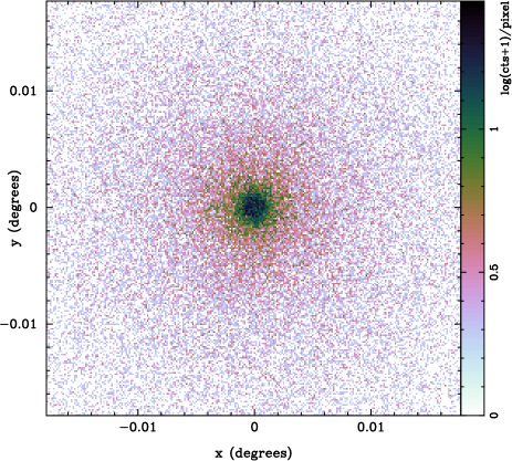
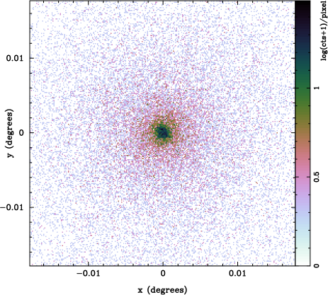
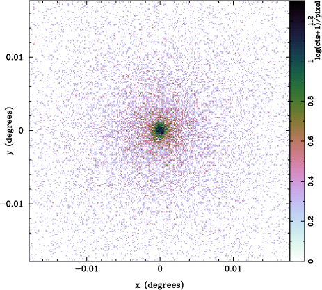
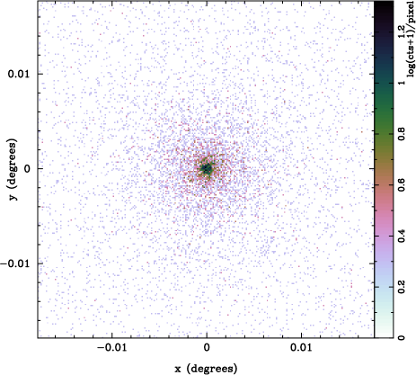
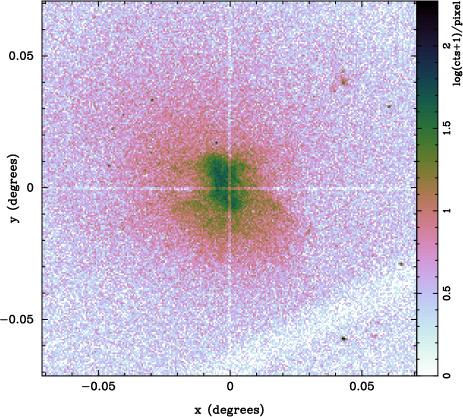
For illustration purposes we have also generated the X-ray images of the simulated clusters. Fig. 1 shows the X-ray maps of the clusters in our sample where we have used ‘cubehelix’ colour scheme (Green, 2011) to display the counts maps. The maps are bolometric maps where we have summed the counts over energy channels at each pixel. Also the maps are in logarithmic scale. From the maps it is clear that as the cluster redshift increases, the cluster X-ray signal becomes fainter, as expected.

6 Bayesian analysis of X-ray clusters using Bayes-X

We adopt model I to calculate the X-ray 3-D predicted count rates, $\left[C^{s}_{lm}\right]^{i}_{pred}$. This requires the knowledge of (a) parameters describing the plasma density and its temperature, namely $R_{\rm s}$, $\rho_{\rm s}$, $r_{\rm p}$, and $P_{\rm{ei}}$; (b) X-ray emissivity and photoelectric absorption cross-sections; and (c) background and telescope response files.

Our sampling parameter space comprises of $\mbox{\boldmath$\Theta$}_{\rm c}\equiv(x_{\rm 0},y_{\rm 0},M_{\rm{T}}(r_{200}),f_{\rm g}(r_{200}),z,c_{500},a,b,c)$, where $x_{\rm 0}$ and $y_{\rm 0}$ are cluster projected position on the sky. To this we can add the parameters describing the background model. We further assume that the priors on sampling parameters are separable (Feroz et al., 2009) such that

$$\pi(\mbox{\boldmath$\Theta$}_{\rm c}) = \pi(x_{\rm 0})\,\pi(y_{\rm 0})\,\pi(M_{\rm T}(r_{\rm 200}))\pi(f_{\rm g}(r_{\rm{200}}))\pi(z)\times$$ (25)

$$\pi(c_{500})\pi(a)\,\pi(b)\,\pi(c).$$

By sampling from $M_{\rm{T}}(r_{\rm 200})$, $z$ and $c_{500}$ Bayes-X calculates $R_{\rm s}$, $\rho_{\rm s}$ and $r_{\rm p}$ assuming spherical geometry and using equation (18). By sampling from $M_{\rm{T}}(r_{\rm 200})$ and $f_{\rm{g}}(r_{\rm 200})$ it also calculates $M_{\rm{g}}(r_{\rm 200})=f_{\rm{g}}(r_{\rm 200})M_{\rm{T}}(r_{\rm 200})$. Using $M_{\rm{g}}(r_{\rm 200})$ it determines the model parameter $P_{\rm{ei}}$ by sampling from $a$, $b$, $c$, and assumption of hydrostatic equilibrium (for detailed calculation see Olamaie et al. 2012, 2013).

Following the steps described in section 4, Bayes-X then calculates the model map of the X-ray source and background flux density on a grid of $256$ by $256$ and at each energy channel. 3-D predicted count rates and the X-ray likelihood function are estimated using equations (23) and (14) assuming the telescope and background files of data products.

Bayes-X also uses model II assuming an Einasto density profile to determine the X-ray likelihood and constrain cluster physical properties. In this paper we only use model II for model comparison purposes. As is described in appendix A, the Einasto profile has one more parameter,$\alpha$, describing the shape of the profile. In Bayes-X this parameter is assumed to be a sampling parameter. Bayes-X also calculates the natural logarithm of the Bayesian evidence. This allows us to perform the Bayesian model selection by calculating the natural logarithm of the Bayes factor,

$${\rm ln}B_{21}=\Delta{\rm ln}{\mathcal{Z}_{21}}={\rm ln}{\mathcal{Z}_{2}}-{\rm ln}{\mathcal{Z}_{1}},$$ (26)

where ${\rm ln}{\mathcal{Z}_{2}}$ is the natural logarithm of the Bayesian evidence for model II assuming Einasto density profile and ${\rm ln}{\mathcal{Z}_{1}}$ is the natural logarithm of the Bayesian evidence for model I assuming the NFW density profile. This naturally penalises the Einasto model for additional parameter, and so takes into account the decrease in number of degrees of freedom.

6.1 Bayes-X analysis of simulated X-ray clusters

Using Bayes-X, we study the sample of four simulated X-ray clusters with the input parameters as given in Tables 2 and 3. We perform four sets of analyses (I, II, III, IV) and also analyses with no-data using model I first in order to investigate the capability of the data, our model and the analysis to return the simulated cluster quantities and clearly reveal structure of degeneracies in the cluster parameter space.

A summary of the priors on the sampling parameters in the analyses I–IV for model I is presented in Table 4. We use Gaussian priors on cluster position parameters, centred on the pointing centre and with standard-deviation of $4^{\arcsec}$. We adopt a $\delta$-function prior on redshift $z$ at the true value for each cluster. The prior on $M_{\rm{T}}(r_{\rm 200})$ is taken to be uniform in log$M$ in the range $M_{\rm{min}}=10^{14}\,\rm{M_{\odot}}$ to $M_{\rm{max}}=6\times 10^{15}\,\rm{M_{\odot}}$. The prior on $f_{\rm{g}}(r_{\rm 200})$ is set to be a Gaussian centred at $f_{\rm{g}}=0.13$ with a width of $0.02$ in the analyses I, III, IV and in the no-data analysis and uniform with a wide range between $0.01$ and $1.0$ in analysis II.

We fix the values of $(c_{500},a,b,c)$ in the analyses I and II to the input values of the simulated clusters given in Table 3 and appendix B in Arnaud et al. (2010).

  

Figure 2: Chandra ACIS-S images (on a logarithmic colour scale) of A262 in the $0.7-7$ keV energy band. top: the left image is produced with a bin size of $2^{\arcsec}$ and the right image is with $16^{\arcsec}$ binning. bottom: blank-sky observation within the same energy range. North is up and east is to the left.

$z=0.5$

    

Figure 3: Analysis I: 2-D and 1-D marginalised posterior distributions of sampling parameters (left) and derived parameters (right) of the X-ray simulated cluster at redshift $z=0.5$. The priors used for the analysis are given in the first column of Table 4.The vertical green solid lines on the 1-D posterior distributions of the parameters show the input values used to generate the simulated cluster and the dashed magenta lines are the mean values of the distributions. $x_{0}$ and $y_{0}$ are in arcsec. $M$ and $f_{\rm g}$ stand for $M_{\rm{T}}(r_{200})$ and $f_{\rm g}(r_{200})$ respectively. $M$ is in $\rm{M_{\odot}}$

Table 5: Mean and 68$\%$-confidence uncertainties of sampling and derived parameters of simulated cluster 1 assuming model I.

Cluster 1	Input	Analysis
Parameters	values	I	II	III	IV
$x_{0}$(arcsec)	$0$	$-0.03^{+0.06}_{-0.06}$	$-0.03^{+0.06}_{-0.11}$	$-0.030^{+0.004}_{-0.110}$	$-0.03^{+0.06}_{-0.05}$
$y_{0}$(arcsec)	$0$	$0.05^{+0.06}_{-0.06}$	$0.05^{+0.06}_{-0.06}$	$0.05^{+0.06}_{-0.06}$	$0.05^{+0.06}_{-0.06}$
$M_{\rm T}(r_{200}){\times}10^{14}\rm{M_{\odot}}$	$6.16$	$6.1^{+0.1}_{-0.1}$	$6.1^{+0.1}_{-0.1}$	$6.2^{+0.2}_{-0.2}$	$6.2^{+0.2}_{-0.2}$
$f_{\rm g}(r_{200})$	$0.13$	$0.129^{+0.001}_{-0.001}$	$0.128^{+0.001}_{-0.001}$	$0.12^{+0.01}_{-0.01}$	$0.12^{+0.01}_{-0.01}$
$a$	$1.0620$	$1.0620$	$1.0620$	$1.06^{+0.02}_{-0.02}$	$1.06^{+0.06}_{-0.06}$
$b$	$5.4807$	$5.4807$	$5.4807$	$5.4^{+0.3}_{-0.3}$	$5.7^{+1.9}_{-1.7}$
$c$	$0.3292$	$0.3292$	$0.3292$	$0.329^{+0.005}_{-0.005}$	$0.33^{+0.01}_{-0.01}$
$c_{500}$	$1.156$	$1.156$	$1.156$	$1.15^{+0.02}_{-0.02}$	$1.2^{+0.5}_{-0.5}$
$M_{\rm T}(r_{500}){\times}10^{14}\rm{M_{\odot}}$	$4.56$	$4.5^{+0.1}_{-0.1}$	$4.5^{+0.1}_{-0.1}$	$4.5^{+0.2}_{-0.2}$	$4.5^{+0.2}_{-0.2}$
$f_{\rm g}(r_{500})$	$0.119$	$0.118^{+0.001}_{-0.001}$	$0.118^{+0.001}_{-0.001}$	$0.118^{+0.006}_{-0.006}$	$0.118^{+0.007}_{-0.007}$
$r_{500}$(Mpc)	$1.098$	$1.09^{+0.01}_{-0.01}$	$1.09^{+0.01}_{-0.01}$	$1.09^{+0.01}_{-0.01}$	$1.09^{+0.01}_{-0.01}$
$M_{\rm g}(r_{500}){\times}10^{13}\rm{M_{\odot}}$	$5.47$	$5.39^{+0.07}_{-0.07}$	$5.39^{+0.07}_{-0.07}$	$5.4^{+0.1}_{-0.1}$	$5.4^{+0.2}_{-0.2}$
$T_{\rm g}(r_{500})$(keV)	$3.45$	$3.42^{+0.05}_{-0.05}$	$3.42^{+0.05}_{-0.05}$	$3.4^{+0.1}_{-0.1}$	$3.5^{+0.3}_{-0.3}$
$r_{200}$(Mpc)	$1.65$	$1.64^{+0.01}_{-0.01}$	$1.64^{+0.01}_{-0.01}$	$1.64^{+0.02}_{-0.02}$	$1.64^{+0.02}_{-0.02}$
$M_{\rm g}(r_{200}){\times}10^{13}\rm{M_{\odot}}$	$8.0$	$7.9^{+0.1}_{-0.1}$	$7.9^{+0.1}_{-0.1}$	$7.9^{+0.4}_{-0.4}$	$7.9^{+0.6}_{-0.6}$
$T_{\rm g}(r_{200})$(keV)	$2.8$	$2.77^{+0.04}_{-0.04}$	$2.77^{+0.04}_{-0.04}$	$2.8^{+0.1}_{-0.1}$	$2.8^{+0.4}_{-0.4}$
$c_{200}$	$3.78$	$3.79^{+0.01}_{-0.01}$	$3.79^{+0.01}_{-0.01}$	$3.79^{+0.01}_{-0.01}$	$3.79^{+0.01}_{-0.01}$

In analysis III we use Gaussian priors on $(c_{500},a,b,c)$ centred on the input values of the simulated clusters with standard deviations as given in the third column of Table 4. The widths on the Gaussian priors were chosen to ensure no singularity in the GNFW pressure profile. As well as analysing the simulated data we also perform a prior-only analysis assuming this set of prior probability distributions.

Finally, in analysis IV we use uniform priors on $(c_{500},a,b,c)$ with the ranges as given in fourth column of Table 4. We adopt the range according to the studies carried out by Arnaud et al. (2010) and Planck Collaboration et al. (2013). Arnaud et al. (2010) studied $31$ Representative XMM-Newton Cluster Structure Survey (REXCESS) cluster sample from XMM-Newton observations (Böhringer et al., 2007; Pratt et al., 2010; Arnaud et al., 2010) within $r_{500}$. They fitted each individual observed cluster pressure profile with the GNFW model, fixing $b=5.4905$. The range of the estimated best fitting parameters for this cluster sample are: $0.01\leq c_{500}\leq 5.51$, $0.33\leq a\leq 2.54$ and $0.0\leq c\leq 1$. Planck Collaboration et al. 2013 also studied the pressure profiles of $62$ nearby massive clusters detected at high significance in the $14$-month nominal survey using a GNFW pressure profile. Their cluster sample is a sub-sample from the ESZ catalogue (The Early release SZ sample) which comprises $189$ clusters detected in SZ (Planck Collaboration et al., 2011). They fixed the value of $c=0.31$ and derived the best fit values for the other three parameters for each individual cluster in their sample. Their parameter values lie in $0.01\leq c_{500}\leq 5.51$, $0.36\leq a\leq 10$ and $2.23\leq b\leq 15$. We therefore selected the range of the priors on $(c_{500},a,b,c)$ according to the minimum and maximum values of the best fitting values in these two studies rounding the numbers to the nearest integers in case of $c_{500}$ and $b$. Similar to analysis III we also performed a prior-only analysis assuming this set of priors.

For model selection purposes we perform the same analyses using model II to calculate the Bayesian evidence. Model II has one more sampling parameter, $\alpha$. As shown in Gao et al. (2008), the best fit values for $\alpha$ spans in the range of $0.12<\alpha<0.25$. To accommodate such a range comfortably, we assume a uniform prior on $\alpha$ between $0.05$ and $0.5$.

6.2 Bayes-X analysis of Abell 262

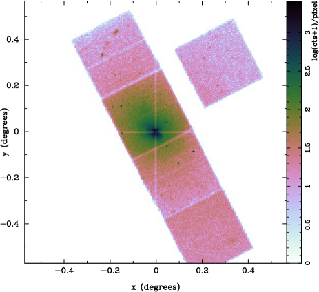
A262 (RA= $01:52:46.299$, Dec= $+36:09:11.80$) is a bright, nearby poor cluster at $z=0.0162$ (Struble & Rood, 1999) with mean ICM temperature $\approx 2$ keV( see e.g. Vikhlinin et al. 2005, Vikhlinin et al. 2006, Sato, Matsushita, & Gastaldello 2009 and Sanders et al. 2010). Due to its low mass and temperature, it may be considered as an intermediate between clusters and groups. A262 was observed for $110.7$ks in ACIS-S and a blank-sky observation of $450$ks was used for the background fitting. We used dmcopy tool in CIAO: Chandra’s data analysis system (Fruscione et al., 2006) to restrict the energy range to $0.7-7$keV for both imaging and spectral analysis in all of the four data product files: event file, blank-sky observation, $RMF$ and $ARF$. This reduced the number of PI channels to $433$. Also, since the output of CIAO is in fits format, we used ftools-fv to export the event and background files as ASCII files. We then performed a $2^{\arcsec}$ binning to both the event and the background files to generate the 3-dimensional data cubes for the spectral analysis without having to re-group the energy and PI columns. We used our in-house binning software tool for binning the data; this software is also available in the online package. This reduced the size of the data to a manageable level without adversely affecting the subsequent inference of the cluster. The output is a photon counts in a grid of $256\times 256\times 433$ to be read in by Bayes-X. Our Bayesian framework also allows us to analyse the data from one CCD. The X-ray images (Fig.2) were then generated by summing up the counts at each pixel. To illustrate the large scale features in the image we also binned the events with a cellsize of $16^{\arcsec}$ (right pannel of Fig.2). It should be noted that the images are for illustration purposes only. We applied the rmfimg tool in CIAO to convert and expand $RMF$ and $ARF$ files into 2-dimensional images(matrices) for the spectral analysis. Similarly, we used ftools-fv to export the 2-dimensional $RMF$ and $ARF$ as ASCII files to be read in by Bayes-X.

We used model I to analyse A262. We adopted Gaussian priors on cluster position parameters, centred on the pointing centre and with standard-deviation of $4^{\arcsec}$. The prior on the cluster redshift was a $\delta$-function at $z=0.0162$. Since A262 is a very poor cluster, the prior on $M_{\rm{T}}(r_{\rm 200})$ is taken to be uniform in log$M$ in the range $M_{\rm{min}}=10^{12}\,\rm{M_{\odot}}$ to $M_{\rm{max}}=5\times 10^{14}\,\rm{M_{\odot}}$ and the prior on $f_{\rm{g}}(r_{\rm 200})$ is set to be a uniform with a range between $0.01$ and $0.2$ in the analysis. We fix the values of $(c_{500},a,b,c)$ to the values given in (Arnaud et al., 2010). These values have proved a good fit to nearby clusters such as REXCESS sample. We also carried out the analysis with varying $(c_{500},a,b,c)$ but there was no difference in the inferred cluster parameters. The background level at each pixel, the hydrogen column density and the metalicity are also assumed to be constant (see table 2) in this analysis.

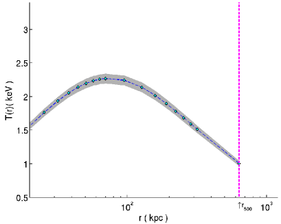
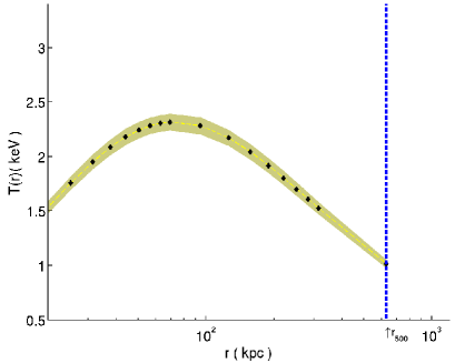
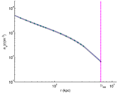
Bayes-X constrains the cluster inferred physical properties at each radius individually provided that the data extend to those radii. Thus, to determine the radial profiles of the inferred physical properties of A262, we calculated the cluster parameters at two overdisity radii of $r_{2500}$ and $r_{500}$ as well as in $15$ different radii spanning the range $0.04r_{500}$ to $0.4r_{500}$. This is the radial extent that our A262 X-ray data can constrain. Included in the output there are two files: A262outstats.dat and A262.txt. A262outstats.dat contains the mean and standard deviation of the inferred parameters and A262.txt contains the entire posterior distribution of the inferred parameters. We use the GETDIST package both to plot the marginalised posterior distribution of the cluster parameters and to obtain the lower and upper values of the parameters within $68\%$ and $9\%5$ confidence intervals. We use these values to plot the radial profiles of the inferred cluster parameters.

For model selection purposes we also analysed A262 using model II and calculated the evidences for both models. The prior on the Einasto shape parameter, $\alpha$, was the same as the one assumed in analysing the X-ray simulated data, i.e. uniform between 0.05 and 0.5.

$z=0.5$

    

Figure 4: Analysis II: 2-D and 1-D marginalised posterior distributions of sampling parameters (left) and derived parameters (right) of the X-ray simulated cluster at redshift $z=0.5$. The priors are given in the second column of Table 4. In this analysis, the prior on $f_{\rm g}(r_{200})$ is assumed to be uniform between $0.01$ and $1$. The vertical green solid lines on the 1-D posterior distributions of the parameters show the input values used to generate the simulated cluster and the dashed magenta lines are the mean values of the distributions. $x_{0}$ and $y_{0}$ are in arcsec. $M$ and $f_{\rm g}$ stand for $M_{\rm{T}}(r_{200})$ and $f_{\rm g}(r_{200})$ respectively. $M$ is in $\rm{M_{\odot}}$

Table 6: Mean and 68$\%$-confidence uncertainties of sampling and derived parameters of simulated cluster 2 assuming model I.

Cluster 2	Input	Analysis
Parameters	values	I	II	III	IV
$x_{0}$(arcsec)	$0$	$-0.07^{+0.06}_{-0.06}$	$-0.07^{+0.06}_{-0.06}$	$-0.07^{+0.06}_{-0.06}$	$-0.07^{+0.06}_{-0.06}$
$y_{0}$(arcsec)	$0$	$0.08^{+0.06}_{-0.06}$	$0.08^{+0.06}_{-0.06}$	$0.07^{+0.06}_{-0.06}$	$0.07^{+0.06}_{-0.06}$
$M_{\rm T}(r_{200})\times 10^{14}\rm{M_{\odot}}$	$5.80$	$5.9^{+0.2}_{-0.2}$	$5.9^{+0.2}_{-0.2}$	$6.0^{+0.2}_{-0.2}$	$6.0^{+0.3}_{-0.3}$
$f_{\rm g}(r_{200})$	$0.13$	$0.127^{+0.002}_{-0.002}$	$0.126^{+0.002}_{-0.002}$	$0.12^{+0.01}_{-0.01}$	$0.12^{+0.01}_{-0.01}$
$a$	$1.0620$	$1.0620$	$1.0620$	$1.07^{+0.02}_{-0.02}$	$1.11^{+0.06}_{-0.06}$
$b$	$5.4807$	$5.4807$	$5.4807$	$5.57^{+0.25}_{-0.24}$	$5.4^{+1.8}_{-1.6}$
$c$	$0.3292$	$0.3292$	$0.3292$	$0.336^{+0.006}_{-0.006}$	$0.34^{+0.01}_{-0.01}$
$c_{500}$	$1.156$	$1.156$	$1.156$	$1.15^{+0.02}_{-0.02}$	$1.3^{+0.5}_{-0.6}$
$M_{\rm T}(r_{500})\times 10^{14}\rm{M_{\odot}}$	$4.3$	$4.4^{+0.1}_{-0.1}$	$4.4^{+0.1}_{-0.1}$	$4.5^{+0.2}_{-0.2}$	$4.5^{+0.2}_{-0.2}$
$f_{\rm g}(r_{500})$	$0.1208$	$0.117^{+0.001}_{-0.001}$	$0.117^{+0.001}_{-0.001}$	$0.115^{+0.005}_{-0.005}$	$0.115^{+0.006}_{-0.006}$
$r_{500}$(Mpc)	$1.038$	$1.04^{+0.01}_{-0.01}$	$1.04^{+0.01}_{-0.01}$	$1.05^{+0.01}_{-0.01}$	$1.05^{+0.01}_{-0.01}$
$M_{\rm g}(r_{500})\times 10^{13}\rm{M_{\odot}}$	$5.19$	$5.18^{+0.08}_{-0.08}$	$5.18^{+0.08}_{-0.08}$	$5.1^{+0.1}_{-0.1}$	$5.1^{+0.1}_{-0.1}$
$T_{\rm g}(r_{500})$(keV)	$3.40$	$3.43^{+0.06}_{-0.06}$	$3.43^{+0.06}_{-0.06}$	$3.4^{+0.1}_{-0.1}$	$3.5^{+0.4}_{-0.4}$
$r_{200}$(Mpc)	$1.557$	$1.56^{+0.01}_{-0.01}$	$1.56^{+0.01}_{-0.01}$	$1.57^{+0.02}_{-0.02}$	$1.57^{+0.02}_{-0.02}$
$M_{\rm g}(r_{200})\times 10^{13}\rm{M_{\odot}}$	$7.54$	$7.5^{+0.1}_{-0.1}$	$7.5^{+0.1}_{-0.1}$	$7.4^{+0.3}_{-0.3}$	$7.4^{+0.5}_{-0.5}$
$T_{\rm g}(r_{200})$(keV)	$2.79$	$2.81^{+0.05}_{-0.05}$	$2.80^{+0.05}_{-0.05}$	$2.8^{+0.1}_{-0.1}$	$2.9^{+0.4}_{-0.4}$
$c_{200}$	$3.52$	$3.51^{+0.01}_{-0.01}$	$3.51^{+0.01}_{-0.01}$	$3.50^{+0.01}_{-0.01}$	$3.50^{+0.01}_{-0.01}$

$z=0.5$

    

Figure 5: Analysis III: 2-D and 1-D marginalised posterior distributions of sampling parameters (left) and derived parameters (right) of the X-ray simulated cluster at redshift $z=0.5$. The priors used for the analysis are given in third column of Table 4.The vertical green solid lines on the 1-D posterior distributions of the parameters show the input values used to generate the simulated cluster and the dashed magenta lines are the mean values of the distributions. $x_{0}$ and $y_{0}$ are in arcsec. $M$ and $f_{\rm g}$ stand for $M_{\rm{T}}(r_{200})$ and $f_{\rm g}(r_{200})$ respectively. $M$ is in $\rm{M_{\odot}}$.

    

Figure 6: 1-D marginalised posterior distributions of sampling parameters (left) and derived parameters (right) of the no-data run (black solid lines) and X-ray simulated cluster 3 at redshift $z=0.5$ (blue solid lines). The priors used for the analysis are given in the third column of Table 4.

$z=0.5$

    

Figure 7: Analysis IV: 2-D and 1-D marginalised posterior distributions of sampling parameters (left) and derived parameters (right) of the X-ray simulated clusters at redshift $z=0.5$. The priors used for the analysis are given in fourth column of Table 4.The vertical green solid lines on the 1-D posterior distributions of the parameters show the input values used to generate the simulated cluster and the dashed magenta lines are the mean values of the distributions. $x_{0}$ and $y_{0}$ are in arcsec. $M$ and $f_{\rm g}$ stand for $M_{\rm{T}}(r_{200})$ and $f_{\rm g}(r_{200})$ respectively. $M$ is in $\rm{M_{\odot}}$.

    

Figure 8: 1-D marginalised posterior distributions of sampling parameters (left) and derived parameters (right) of the no-data run (black solid lines) and simulated Chandra cluster 3 at redshift $z=0.5$ (blue solid lines). The priors used for the analysis are given in fourth column of Table 4.

Table 7: Mean and 68$\%$-confidence uncertainties of sampling and derived parameters of simulated cluster 3 assuming model I.

Cluster 3	Input	Analysis
Parameters	values	I	II	III	IV
$x_{0}$(arcsec)	$0$	$0.04^{+0.07}_{-0.07}$	$0.04^{+0.07}_{-0.07}$	$0.04^{+0.06}_{-0.06}$	$0.04^{+0.06}_{-0.06}$
$y_{0}$(arcsec)	$0$	$0.06^{+0.07}_{-0.07}$	$0.06^{+0.07}_{-0.07}$	$0.06^{+0.07}_{-0.07}$	$0.07^{+0.06}_{-0.06}$
$M_{\rm T}(r_{200})\times 10^{14}\rm{M_{\odot}}$	$5.2$	$5.4^{+0.2}_{-0.2}$	$5.4^{+0.2}_{-0.2}$	$5.4^{+0.3}_{-0.3}$	$5.4^{+0.3}_{-0.3}$
$f_{\rm g}(r_{200})$	$0.13$	$0.126^{+0.002}_{-0.002}$	$0.126^{+0.002}_{-0.002}$	$0.128^{+0.007}_{-0.008}$	$0.13^{+0.01}_{-0.01}$
$a$	$1.062$	$1.062$	$1.062$	$1.05^{+0.03}_{-0.02}$	$1.05^{+0.08}_{-0.08}$
$b$	$5.4807$	$5.4807$	$5.4807$	$5.4^{+0.2}_{-0.2}$	$6.3^{+2.6}_{-2.3}$
$c$	$0.3292$	$0.3292$	$0.3292$	$0.32^{+0.01}_{-0.01}$	$0.32^{+0.01}_{-0.01}$
$c_{500}$	$1.156$	$1.156$	$1.156$	$1.15^{+0.02}_{-0.02}$	$1.2^{+0.6}_{-0.60}$
$M_{\rm T}(r_{500})\times 10^{14}\rm{M_{\odot}}$	$3.85$	$4.0^{+0.1}_{-0.1}$	$4.0^{+0.1}_{-0.1}$	$3.9^{+0.2}_{-0.2}$	$3.9^{+0.2}_{-0.2}$
$f_{\rm g}(r_{500})$	$0.122$	$0.119^{+0.002}_{-0.002}$	$0.118^{+0.002}_{-0.002}$	$0.120^{+0.005}_{-0.005}$	$0.120^{+0.006}_{-0.006}$
$r_{500}$(Mpc)	$0.927$	$0.93^{+0.01}_{-0.01}$	$0.93^{+0.01}_{-0.01}$	$0.93^{+0.01}_{-0.01}$	$0.93^{+0.02}_{-0.02}$
$M_{\rm g}(r_{500})\times 10^{13}\rm{M_{\odot}}$	$4.72$	$4.7^{+0.1}_{-0.1}$	$4.7^{+0.1}_{-0.1}$	$4.7^{+0.1}_{-0.1}$	$4.7^{+0.1}_{-0.1}$
$T_{\rm g}(r_{500})$(keV)	$3.35$	$3.42^{+0.08}_{-0.08}$	$3.42^{+0.08}_{-0.08}$	$3.4^{+0.1}_{-0.1}$	$3.4^{+0.3}_{-0.3}$
$r_{200}$(Mpc)	$1.39$	$1.40^{+0.02}_{-0.02}$	$1.41^{+0.02}_{-0.02}$	$1.40^{+0.02}_{-0.02}$	$1.40^{+0.02}_{-0.02}$
$M_{\rm g}(r_{200})\times 10^{13}\rm{M_{\odot}}$	$6.76$	$6.8^{+0.1}_{-0.1}$	$6.8^{+0.1}_{-0.1}$	$6.8^{+0.2}_{-0.2}$	$6.8^{+0.4}_{-0.4}$
$T_{\rm g}(r_{200})$(keV)	$2.8$	$2.86^{+0.07}_{-0.07}$	$2.86^{+0.07}_{-0.07}$	$2.8^{+0.1}_{-0.1}$	$2.8^{+0.4}_{-0.4}$
$c_{200}$	$3.08$	$3.07^{+0.01}_{-0.01}$	$3.07^{+0.01}_{-0.01}$	$3.07^{+0.01}_{-0.01}$	$3.07^{+0.02}_{-0.02}$

7 Results

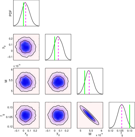
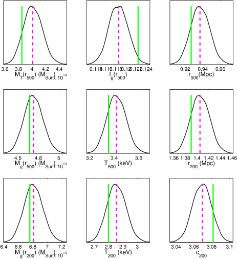
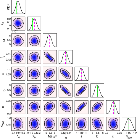
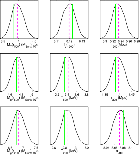
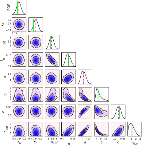
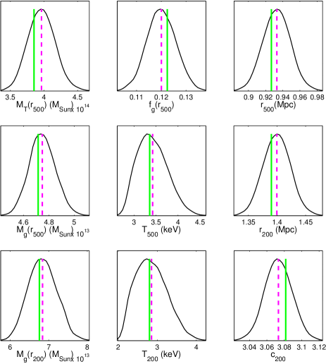
Figs. 3– 8 show 2-D and 1-D marginalised posterior distributions of both sampling and derived parameters of simulated Chandra cluster data at $z=0.5$ for the analyses I–IV as well as 1-D marginalised posterior distributions of prior-only analyses for this cluster. They are the results obtained using model I. The green solid lines on the 1-D posterior distributions of the parameters in Figs 3, 4, 5 and 7 show the input values used to generate the simulated cluster and magneta dashed lines show the mean of the distributions. We note that the general shape of the 2-D and 1-D marginal distributions for all other clusters in the sample are similar. However, we have presented the detailed parameter constraints for each cluster in Tables 5-8.

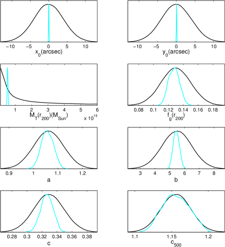
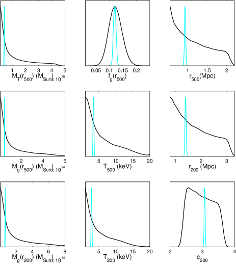
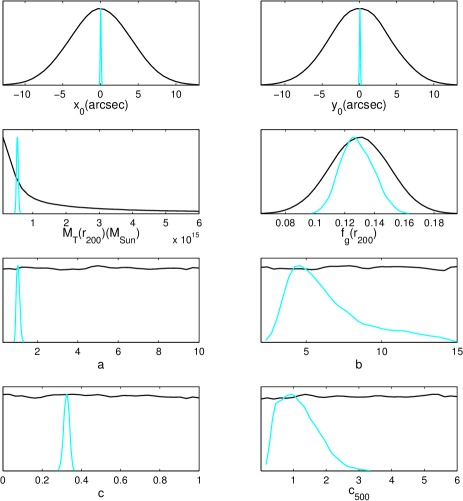
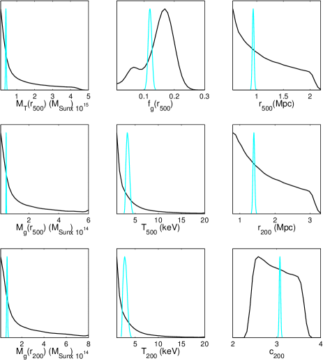
Figs 6 and 8 represent the results of a prior-only analysis showing 1-D marginalised posterior distributions of both sampling and derived parameters (black solid lines) for the simulated cluster at $z=0.5$ assuming model I. Fig. 6 shows the results when we adopted Gaussian priors on $(c_{500},a,b,c)$ according to column three in Table 4. Fig. 8 shows the results when we adopted uniform priors on these parameters as given in column four of Table 4. In both analyses, we fixed the redshift to $z=0.5$ corresponding to the redshift of cluster 3. We have also plotted the 1-D marginalised posterior distributions of both sampling and derived parameters (blue solid lines) of cluster 3 in both figures.

As described in section 6, one of the output results of Bayes-X is the natural logarithm of the Bayesian evidence. We use equation (26) to calculate the natural logarithm of the Bayes factor for the simulated clusters using models I and II. We find ${\rm ln}B_{21}=-30$ which suggests decisive evidence in favour of model I. This is of course an expected result as we used model I in generating the X-ray simulated clusters.

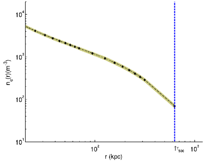
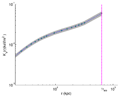
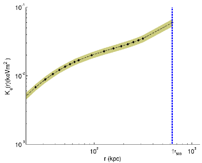
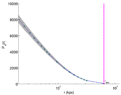
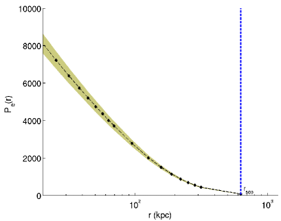
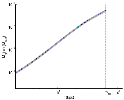
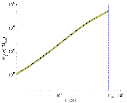
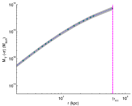
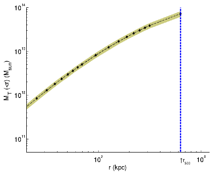
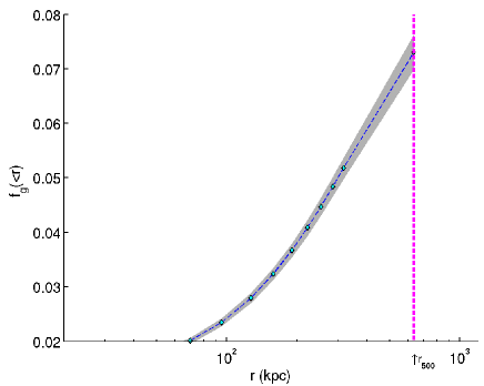
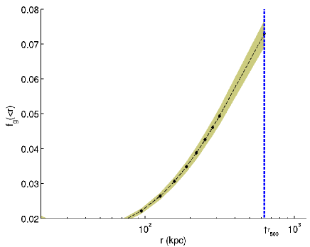
The results of Bayes-X analysis for A262 assuming model I and II are shown in Figs. 9 and 10. The plots represent the radial profiles of the physical properties of A262 including ICM temperature, electron number density, entropy, integrated gas mass, total mass and gas mass fraction out to $r_{500}$. The cyan and black diamond points are the inferred parameter mean values at $15$ different radii spanning the range $0.04r_{500}$ – $0.4r_{500}$. The grey and yellow shaded areas represent 68$\%$ confidence uncertainity and the vertical magenta and balck dashed line is radius $r_{500}$. The means and standard deviations ($\sigma$) of the parameters are calculated from the posterior samples provided from MultiNest. Table 9 presents the detailed parameter constraints for this cluster at two overdensity coefficients, $\Delta=2500$ and $\Delta=500$ using model I. The results of the model comparison for A262 decisively favours model II with ${\rm ln}B_{21}=45$.

8 Discussion

From the plots described above we note that the cluster position ($x_{0}$ and $y_{0}$) on the sky is firmly constrained in all cases and the true values all lie within $1\sigma$ of the means of the posterior probability distributions.

Throughout the analyses, the tight constraints on $M_{\rm g}$, $T_{\rm g}$ and $M_{\rm{T}}$ and their insensitivity to the choice of priors are also clear, which shows the strong correlation between the X-ray luminosity and the cluster mass.

Similarly, from the 1-D marginalised posterior distributions of both $f_{\rm g}(r_{200})$ and $f_{\rm g}(r_{500})$, it is clear that we are able to constrain $f_{\rm g}$ even in the analysis II where we assume a wide prior on $f_{\rm g}(r_{200})$. The negative degeneracy between $f_{\rm g}$ and $M_{\rm{T}}$ is also apparent in the corresponding 2-D marginalised probability distributions in all the analyses, as one would expect ($f_{\rm g}=M_{\rm{g}}/M_{\rm{T}}$).

In order to investigate the capability of our simulated X-ray data and analysis pipeline to constrain parameters describing the shape and slopes of the GNFW model, namely ($c_{500},a,b,c$), and to return the simulated cluster input values we let these parameters vary in the analyses III and IV. As was mentioned in section 6.1, we first assumed Gaussian prior probability distributions on these parameters centred on the input values used to generate the simulated clusters and with narrow widths (see third column in Table 4). Fig.5 shows the results of the analysis. Then in order to make sure that the results are not biased by the narrow Gaussian prior distributions, and to reveal the degeneracy between the parameters more clearly, we assume uniform priors on the pressure profile shape and slope parameters in analysis IV. We selected the range of priors based on the studies in Arnaud et al. (2010) and Planck Collaboration et al. (2013) (see fourth column in Table 4). Fig.7 shows the results of the analysis. From the plots we note that the simulated X-ray data can constrain the cluster model parameters and recover the input true values. This confirms that X-ray data can probe the cluster core and constrain the shape and slope parameters of the plasma pressure profile.

The 2-D marginalised posterior probability distributions of ($c_{500},a,b,c$) also show clear degeneracies among these parameters. This implies that obtaining an unbiased estimate of cluster parameters requires taking into account the degeneracies among these parameters in the analysis which can only be achieved by letting all four parameters vary.

There is also no correlation between the values of the physical parameter, $M_{\rm{T}}$, and the shape parameters, $a$, $b$ and $c$. Further, the mean values of the cluster parameters do not change significantly upon changing the prior probability distributions in different analyses.

We have also investigated our methodology in the absence of data when we sample from the whole set of parameters, namely $\mbox{\boldmath$\Theta$}_{\rm c}\equiv(x_{\rm 0},y_{\rm 0},M_{\rm{T}}(r_{200}),f_{\rm g}(r_{200}),z,c_{500},a,b,c)$. This is carried out by setting the likelihood to a constant value and hence the algorithm explores the prior space. This analysis is crucial for understanding the underlying biases and constraints imposed by the priors and the model assumptions. The comparison of this analysis with the analysis using the simulated Chandra data reveals the constraints that measurements of the X-ray signal place on the cluster physical parameters and the robustness of the assumptions made.

Figs 6 and 8 represent the results of the prior-only analysis showing 1-D marginalised posterior distributions of both sampling and derived parameters (black solid lines). The results not only show that we are able to recover the assumed prior probability distributions of cluster parameters but also demonstrate the tight constraints on the cluster parameters arising from the simulated X-ray data. We note that the constraint on $c_{500}$ in Fig.6 from the simulated X-ray data overlaps the one from the no-data run but as Fig.8 shows this effect is a direct result of imposing a tight and very informative prior on $c_{500}$.

We also note the tight constraints that these simulated X-ray data sets can place upon the $c$ and $a$ parameters, which describe the slopes of the GNFW pressure profile at $r\ll r_{\rm p}$ and $r\approx r_{\rm p}$ and the fairly wide constraint on the $b$ parameter that describes the slope where $r>r_{\rm p}$ (Fig.8).

The results of the Bayesian model selection analysis of simulated data also confirms the robustness of the analysis pipeline as it decisively favours model I as expected.

We then repeat the analysis for the real cluster A262 observed with Chandra. We extract the cluster physical properties as a function of radius out to $r_{500}$ in $15$ different radii assuming model I. As may be seen from the plots in figs. 9 and 10, all the physical properties of A262 follow the distributions as expected, e.g. electron number density decreases with radius while the cluster gas mass and total mass increase. Also, as found in PKS0745 cluster, (Sanders et al., 2014), the bubbles of non-thermal material in the core of A262 generated by the AGN could make the apparent thermal pressure reduce and therefore flatten out the central mass profile. As A262 is a poor cluster, in Table 9, we only present the detailed parameter constraints with their corresponding errors out to overdensities of $\Delta=2500$ and $\Delta=500$.

A262 has been studied using various X-ray telescopes including Chandra, XMM-Newton and Suzaku (see e.g. Vikhlinin et al. 2005, Vikhlinin et al. 2006, Gastaldello et al. 2007, Sato, Matsushita, & Gastaldello 2009, Sun et al. 2009 and Sanders et al. 2010). Overall, the results of the Bayes-X analysis of A262 are in agreement with these studies. For example Vikhlinin et al. (2006) estimate $T_{\mathrm{spec}}=2.08\pm 0.06$keV, $T_{\mathrm{mg}}=1.89\pm 0.09$keV and $r_{500}=650\pm 21$kpc. Sato, Matsushita, & Gastaldello (2009), on the other hand, measure a single mean temperature for the cluster, $k<T>=2.0$keV. The Bayes-X estimate of halo concentration parameter, $c^{\rm{halo}}_{500}$ is also consistent with Vikhlinin et al. (2006) and Sun et al. (2009) within their estimated errors. However, the Bayes-X result for $c^{\rm{halo}}_{2500}$ is smaller than the values quoted by Gastaldello et al. (2007). The Bayes-X estimate of $M_{\rm T}(r_{2500})$ agrees with the result by Vikhlinin et al. (2006) but is smaller than the results by Gastaldello et al. (2007).

The results of the Bayesian model selection for A262 shows decisive evidence strength in favour of model II indicating A262 data prefer Einasto profile. As mentioned in section 6, in the Einasto profile, the shape parameter, $\alpha$ is a free parameter and is a power law function of radius, $\frac{{\rm dln}\rho}{{\rm dln}r}=-2(\frac{r}{r_{-2}})^{\alpha}$. Our Bayes-X best fit value of $\alpha$ is $0.2474\pm 0.0004$. It has also been shown (see e.g. Gao et al. 2008, Navarro et al. 2010, Chemin, de Blok, & Mamon 2011, Retana-Montenegro et al. 2012 and Dutton & Macciò 2014) that the Einasto profile fits the inner cusps better, is consistent with observed rotation curves, and its additional shape parameter varies with mass. The inferred cluster parameters such as masses are, however, in good agreement using both models.

Table 8: Mean and 68$\%$-confidence uncertainties sampling and derived parameters of simulated cluster 4 assuming model I.

Cluster 4	Input	Analysis
Parameters	values	I	II	III	IV
$x_{0}$(arcsec)	$0$	$-0.02^{+0.07}_{-0.07}$	$-0.02^{+0.07}_{-0.07}$	$-0.02^{+0.07}_{-0.07}$	$-0.02^{+0.06}_{-0.06}$
$y_{0}$(arcsec)	$0$	$0.05^{+0.07}_{-0.07}$	$0.05^{+0.07}_{-0.07}$	$0.04^{+0.07}_{-0.06}$	$0.04^{+0.06}_{-0.06}$
$M_{\rm T}(r_{200})\times 10^{14}\rm{M_{\odot}}$	$4.10$	$4.1^{+0.2}_{-0.2}$	$4.1^{+0.2}_{-0.2}$	$4.3^{+0.3}_{-0.3}$	$4.3^{+0.3}_{-0.3}$
$f_{\rm g}(r_{200})$	$0.13$	$0.130^{+0.003}_{-0.003}$	$0.130^{+0.003}_{-0.003}$	$0.120^{+0.008}_{-0.008}$	$0.12^{+0.01}_{-0.01}$
$a$	$1.0620$	$1.0620$	$1.0620$	$1.08^{+0.03}_{-0.03}$	$1.1^{+0.1}_{-0.1}$
$b$	$5.4807$	$5.4807$	$5.4807$	$5.6^{+0.2}_{-0.2}$	$6.2^{+2.9}_{-2.4}$
$c$	$0.329$	$0.3292$	$0.3292$	$0.34^{+0.01}_{-0.01}$	$0.35^{+0.02}_{-0.02}$
$c_{500}$	$1.156$	$1.156$	$1.156$	$1.15^{+0.02}_{-0.02}$	$1.3^{+0.7}_{-0.7}$
$M_{\rm T}(r_{500})\times 10^{14}\rm{M_{\odot}}$	$3.04$	$3.0^{+0.1}_{-0.1}$	$3.0^{+0.1}_{-0.1}$	$3.2^{+0.2}_{-0.2}$	$3.2^{+0.2}_{-0.2}$
$f_{\rm g}(r_{500})$	$0.125$	$0.125^{+0.003}_{-0.003}$	$0.125^{+0.003}_{-0.003}$	$0.119^{+0.006}_{-0.006}$	$0.117^{+0.006}_{-0.006}$
$r_{500}$(Mpc)	$0.73$	$0.73^{+0.01}_{-0.01}$	$0.73^{+0.01}_{-0.01}$	$0.74^{+0.02}_{-0.02}$	$0.74^{+0.02}_{-0.02}$
$M_{\rm g}(r_{500})\times 10^{13}\rm{M_{\odot}}$	$3.8$	$3.7^{+0.1}_{-0.1}$	$3.7^{+0.1}_{-0.1}$	$3.7^{+0.1}_{-0.1}$	$3.7^{+0.1}_{-0.1}$
$T_{\rm g}(r_{500})$(keV)	$3.25$	$3.2^{+0.1}_{-0.1}$	$3.2^{+0.1}_{-0.1}$	$3.2^{+0.1}_{-0.1}$	$3.2^{+0.4}_{-0.4}$
$r_{200}$(Mpc)	$1.1$	$1.09^{+0.02}_{-0.02}$	$1.09^{+0.02}_{-0.02}$	$1.11^{+0.02}_{-0.02}$	$1.11^{+0.02}_{-0.02}$
$M_{\rm g}(r_{200})\times 10^{13}\rm{M_{\odot}}$	$5.33$	$5.3^{+0.1}_{-0.1}$	$5.3^{+0.1}_{-0.1}$	$5.2^{+0.2}_{-0.2}$	$5.2^{+0.3}_{-0.3}$
$T_{\rm g}(r_{200})$(keV)	$2.80$	$2.76^{+0.08}_{-0.08}$	$2.76^{+0.09}_{-0.09}$	$2.7^{+0.1}_{-0.1}$	$2.7^{+0.5}_{-0.5}$
$c_{200}$	$2.49$	$2.49^{+0.01}_{-0.01}$	$2.49^{+0.01}_{-0.01}$	$2.48^{+0.02}_{-0.02}$	$2.48^{+0.02}_{-0.02}$

Table 9: Mean and 68$\%$-confidence uncertainties of the physical properties of A262 for two overdensities $\Delta=2500$ and $\Delta=500$ assuming model I.

A262	$\Delta=2500$	$\Delta=500$
$c^{\rm{halo}}_{\Delta}$	$1.53^{+0.01}_{-0.01}$	$3.57^{+0.01}_{-0.01}$
$r_{\Delta}$(kpc)	$272.4^{+0.5}_{-0.5}$	$635.5^{+1.2}_{-1.2}$
$M_{\rm T}(r_{\Delta})\times 10^{13}(\rm{M_{\odot}})$	$2.92^{+0.02}_{-0.02}$	$7.42^{+0.04}_{-0.04}$
$M_{\rm g}(r_{\Delta})\times 10^{12}(\rm{M_{\odot}})$	$1.51^{+0.01}_{-0.01}$	$5.42^{+0.02}_{-0.02}$
$f_{\rm g}(r_{\Delta})$	$0.052^{+0.001}_{-0.001}$	$0.073^{+0.003}_{-0.003}$
$T_{\rm g}(r_{\Delta})$(keV)	$1.604^{+0.006}_{-0.006}$	$1.004^{+0.004}_{-0.004}$
$n_{\rm e}(r_{\Delta})(\rm{m^{-3}})$	$368.3^{+0.6}_{-0.6}$	$68.8^{+0.1}_{-0.1}$
$K_{\rm e}(r_{\Delta})(\rm{keVm^{2}})$	$0.0312^{+0.0001}_{-0.0001}$	$0.0598^{+0.0003}_{-0.0003}$

model I                                 model II

  

  

  

  

Figure 9: Profiles of temperature, electron number density, entropy as a function of $r$ for A262 using model I(left) and II (right). In each panel, the cyan and black diamonds are the estimated mean values and the grey and the yellow shaded areas show the 68$\%$ confidence levels. The vertical magenta and blue dashed lines show the radius $r_{500}$.

model I                                 model II

  

  

  

Figure 10: Profiles of integrated gas mass, total mass and gas mass fraction as a function of $r$ for A262 using model I(left) and II (right). In each panel, the cyan and black diamonds are the estimated mean values and the grey and the yellow shaded areas show the 68$\%$ confidence levels. The parameters means and standard deviations ($\sigma$) at each point are calculated from the posterior samples provided from MultiNest. The vertical magenta and blue dashed lines show the radius $r_{500}$.

9 Conclusions

By performing a Bayesian analysis of simulated and real Chandra data we have investigated the capability of our model (where we assume that the dark matter density follows a NFW-profile and that the gas pressure is described by a GNFW profile) and Bayes-X to return the cluster input quantities and constrain the cluster physical parameters.

We simulated Chandra-like observations of four clusters in a redshift range of $0.2{-}0.9$ all with the same $f_{\rm g}(r_{200})=0.13$. We have performed four sets of analyses including prior-only analysis and assuming different types of priors on $f_{\rm g}(r_{200})$ and model parameters $(c_{500},a,b,c)$.

We have demonstrated that Bayes-X faithfully recovers the input values of the model parameters used in the simulations and can constrain clusters positions on the sky and clusters physical parameters including $M_{\rm g}$, $T_{\rm g}$ and $M_{\rm T}$.

We find that we can still constrain $f_{\rm g}$ as well as other cluster parameters even when we assume a wide uniform prior on $f_{\rm g}(r_{200})$.

By letting $(c_{500},a,b,c)$ vary in the analysis we have shown that Bayes-X is able to reveal the degeneracy among these parameters which must be taken into account for an unbiased estimate of cluster parameters. We did this by assuming Gaussian and uniform prior probability distributions on $(c_{500},a,b,c)$ respectively. The results also show no correlation between $M_{\rm T}$ and $a$, $b$, or $c$ as one would expect.

The results of prior-only analyses show that we recover the assumed prior probability distributions for cluster positions, model parameters and physical parameters.

We find that the results of the analyses do not depend on the choice of prior probability distributions on the sampling parameters for these high signal-noise simulations and in all cases we were able to recover the input values of the simulated clusters and expected degeneracies among the cluster parameters.

The results of Bayes-X analysis of Chandra data on A262 also show the expected variation of the parameters as a function of radius. The inferred cluster parameters at two overdensities of $\Delta=2500$ and $\Delta=500$ are in general agreement with the results presented in the literature.

The results of the Bayesian model selection favour model I decisively for the X-ray simulated data as expected but prefers model II for A262.

We therefore conclude that Bayes-X is robust and can be used to analyse X-ray data and in future multi-wavelength analysis of clusters of galaxies.

Appendix A Deriving cluster physical properties using model II

In this model we first assume that the cluster matter density follows the Einasto profile,

$$\rho_{\mathrm{Einasto}}(r)=\rho_{\mathrm{-2}}\exp\left\{-\frac{2}{\alpha}\left[\left(\frac{r}{r_{-2}}\right)^{\alpha}-1\right]\right\},$$ (27)

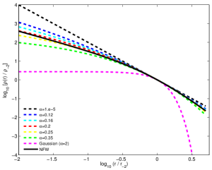
where $r_{-2}$ known as scale radius is the radius where the logarithmic slope of the density profile is $-2$, $\rho_{\mathrm{-2}}$ is the density at the scale radius and $\alpha$ is the shape parameter. The halo concentration parameter is also defined as $c_{200}=\frac{r_{200}}{r_{-2}}$. Figure 11 shows the Einasto density profile for different shape parameter versus NFW density profile.

Figure 11: The Einasto density profile with different $\alpha$. The NFW density profile is shown with black solid line.

As for model I, our second assumption is that $P_{\rm g}(r)$ follows the GNFW profile,

$$P_{\rm e}(r)=\frac{P_{\rm{ei}}}{\left(\frac{r}{r_{\rm p}}\right)^{c}\left(1+\left(\frac{r}{r_{\rm p}}\right)^{a}\right)^{(b-c)/a}}.$$ (28)

The gas pressure is then defined by

$$P_{\rm{g}}(r)=\frac{\mu_{\rm e}}{\mu}P_{\rm{e}}(r).$$ (29)

The third assumption concerns the dynamical state of the cluster, which we take to be in hydrostatic equilibrium throughout. Thus, the total cluster mass internal to radius $r$ is related to the gas pressure gradient at that radius by

$$\frac{{\rm d}P_{\rm{g}}(r)}{{\rm d}r}=-\rho_{\rm{g}}(r)\frac{{\rm G}M(r)}{r^{2}}.$$ (30)

Assuming spherical geometry and using equation 27, the total mass enclosed within radius $r$ has the analytical solution,

$$M(<r) = 4\pi\int_{0}^{r}{r^{\prime 2}\rho_{\mathrm{Einasto}}(r^{\prime})dr^{\prime}}$$ (31)

$$= 4\pi\rho_{\mathrm{-2}}\exp\left(\frac{2}{\alpha}\right)r^{3}_{-2}\left(\frac{\alpha}{2}\right)^{3/\alpha}\frac{1}{\alpha}\mbox{\huge$\Gamma$}\left[\frac{3}{\alpha},\frac{2}{\alpha}\left(\frac{r}{r_{-2}}\right)^{\alpha}\right],$$

where $\mathrm{\Gamma}$ is the lower incomplete gamma function. Substituting this form and the expressions (28) and (29) for the gas pressure into the condition (30) for hydrostatic equilibrium, one may derive the gas density profile

$$\rho_{\rm{g}}(r) = \left(\frac{\mu_{\rm e}}{\mu}\right)\left(\frac{1}{4\pi G}\right)\left(\frac{P_{\rm{ei}}}{\rho_{-2}}\right)\left(\frac{1}{(1/\alpha)(\alpha/2)^{3/\alpha}r_{-2}^{3}\exp(2/\alpha)}\right)\times$$ (32)

$$\frac{r}{\mbox{\huge$\Gamma$}\left[\frac{3}{\alpha},\frac{2}{\alpha}\left(\frac{r}{r_{-2}}\right)^{\alpha}\right]}\times$$

$$\left(\frac{r}{r_{\rm p}}\right)^{{-c}}\left[1+\left(\frac{r}{r_{\rm p}}\right)^{a}\right]^{-\left(\frac{{{a+b-c}}}{{a}}\right)}\left[{b}\left(\frac{r}{r_{\rm p}}\right)^{a}+{c}\right].$$

The radial profile of the electron number density is then trivially obtained using $n_{\rm e}(r)=\rho_{\rm{g}}(r)/\mu_{\rm e}$. Assuming an ideal gas equation of state, this in turn yields the electron temperature profile ${\rm k_{\rm B}}T_{\rm{e}}(r)=P_{\rm e}(r)/n_{\rm e}(r)$, given by

$${\rm k_{\rm B}}T_{\rm{e}}(r) = (4\pi\mu{\rm G}\rho_{-2})(r^{3}_{-2})[(\alpha/2)^{3/\alpha}(1/\alpha)\exp(2/\alpha)]\times$$ (33)

$$\left[\frac{\mbox{\huge$\Gamma$}\left[\frac{3}{\alpha},\frac{2}{\alpha}\left(\frac{r}{r_{-2}}\right)^{\alpha}\right]}{r}\right]\times$$

$$\left[1+\left(\frac{r}{r_{\rm p}}\right)^{a}\right]\left[{b}\left(\frac{r}{r_{\rm p}}\right)^{a}+{c}\right]^{-1}.$$

The only fundamental cluster property for which the radial profile can not be expressed in an explicit analytical form is the gas mass enclosed within radius $r$,

$$M_{\rm{g}}(<r)=\int_{0}^{r}{\rho_{\rm{g}}(r^{\prime})(4\pi r^{\prime 2}{\rm d}r^{\prime})}.$$ (34)

For the gas density profile in (32), we have been unable to evaluate this expression analytically, and so $M_{\rm g}(<r)$ must be obtained using numerical integration. Consequently, the enclosed gas mass fraction profile $f_{\rm{g}}(r)=M_{\rm{g}}(<r)/M(<r)$ also cannot be written in closed form.

Similar to NFW profile, in order to perform the Bayesian analysis and determine the radial profiles of quantities of interest for a given cluster, one must first calculate the values of the model parameters $\rho_{-2},r_{-2},r_{\rm p}$ and $P_{\rm{ei}}$. Bayes-X assumes the same sampling parameters given in equation 25 for model II as well. Thus for a given $M_{\rm{T}}(r_{200})$ and $z$, it calculates $r_{200}$, assuming spherical geometry for the cluster,

$$M_{\rm{T}}(r_{200})=\frac{4\pi}{3}r^{3}_{200}(200\rho_{\rm{crit}}(z)).$$ (35)

$c_{200}$ is also calculated using equation 18 and hence $r_{\rm-2}=r_{200}/c_{200}$. The value of $\rho_{\rm-2}$ is then obtained by equating the input value of $M_{\rm T}(r_{200})$ with the RHS of (31) evaluated at $r=r_{200}$, and is given by

$$\rho_{\rm{-2}}=\frac{200}{3}\left(\frac{r_{200}}{r_{\rm-2}}\right)^{3}\frac{\rho_{\rm{crit}}(z)}{1/\alpha(\alpha/2)^{3/\alpha}\exp(2/\alpha)\mbox{\huge$\Gamma$}\left[\frac{3}{\alpha},\frac{2}{\alpha}\left(\frac{r}{r_{-2}}\right)^{\alpha}\right]}.$$ (36)

By equating equations 31 and 35 at $r_{500}$ and $r_{2500}$, Bayes-X calculates both radii and hence $r_{\rm p}=r_{500}/c_{500}$. Finally, $P_{\rm{ei}}$ is obtained by substituting (32) into (34), evaluating the RHS at $r=r_{200}$ and equating the result to $f_{\rm g}(r_{\rm 200})M_{\rm T}(r_{200})$. This yields

$$P_{\rm{ei}} = \left(\frac{\mu}{\mu_{\rm{e}}}\right)({\rm G}\rho_{\rm{-2}}r^{3}_{\rm-2})\left[1/\alpha(\alpha/2)^{3/\alpha}\exp(2/\alpha)\right]M_{\rm{g}}(r_{200})\times$$ (37)

$$\frac{1}{{\displaystyle\int_{0}^{r_{\rm 200}}}r^{{}^{\prime}3}{\rm d}r^{\prime}\frac{\left[b\left(\frac{r^{\prime}}{r_{\rm p}}\right)^{a}+c\right]}{\mbox{\huge$\Gamma$}\left[\frac{3}{\alpha},\frac{2}{\alpha}\left(\frac{r}{r_{-2}}\right)^{\alpha}\right]\left(\frac{r^{\prime}}{r_{\rm p}}\right)^{c}\left[1+\left(\frac{r^{\prime}}{r_{\rm p}}\right)^{a}\right]^{\left(\frac{{a+b-c}}{a}\right)}}},$$

which is evaluated numerically.

References

- Allen et al. (2008) Allen S. W., Rapetti D. A., Schmidt R. W., Ebeling H., Morris R. G., Fabian A. C., 2008, MNRAS, 383, 879
- Allen, Evrard & Mantz (2011) Allen S. W., Evrard A. E., Mantz A. B., 2011, ARA&A, 49, 409
- AMI Consortium: Hurley-Walker et al. (2012) AMI Consortium: Hurley-Walker et al., 2012, MNRAS, 419, 2921
- AMI Consortium: Olamaie et al. (2012) AMI Consortium: Olamaie et al., 2012, MNRAS, 421, 1136
- Anders & Grevesse (1989) Anders E., Grevesse N., 1989, GeCoA, 53, 197
- Arnaud et al. (2010) Arnaud M., Pratt G. W., Piffaretti R., Böhringer H., Croston J. H., Pointecouteau E., 2010, A &A, 517, A92
- Arnaud et al. (2011) Arnaud, K., Smith, R., & Siemiginowska, A. 2011, Handbook of X-ray Astronomy, by Edited by Keith Arnaud, Randall Smith, Aneta Siemiginowska, Cambridge, UK: Cambridge University Press, 2011,
- Balucinska-Church & McCammon (1992) Balucinska-Church M., McCammon D., 1992, ApJ, 400, 699
- Bartalucci et al. (2014) Bartalucci I., Mazzotta P., Bourdin H., Vikhlinin A., 2014, arXiv:1404.3587
- Bautz et al. (2009) Bautz M. W., et al., 2009, PASJ, 61, 1117
- Böhringer et al. (2007) Bö hringer H. et al., 2007, A&A, 469, 363
- Bonamente et al. (2004) Bonamente M., Joy M. K., Carlstrom J. E., Reese E. D., LaRoque S. J., 2004, ApJ, 614, 56
- Borgani et al. (2004) Borgani S., et al., 2004, MNRAS, 348, 1078
- Borgani (2004) Borgani S., 2004, Ap &SS, 294, 51
- Broos et al. (2010) Broos P. S., Townsley L. K., Feigelson E. D., Getman K. V., Bauer F. E., Garmire G. P., 2010, ApJ, 714, 1582
- Carlberg et al. (1997) Carlberg R. G., et al., 1997, ApJ, 485, L13
- Chemin, de Blok, & Mamon (2011) Chemin L., de Blok W. J. G., Mamon G. A., 2011, AJ, 142, 109
- Corless, King & Clowe (2009) Corless V. L., King L. J., Clowe D., 2009, MNRAS, 393, 1235
- Carter et al. (2003) Carter C., Karovska M., Jerius D., Glotfelty K., Beikman S., 2003, ASPC, 295, 477
- Davis (2001) Davis J. E., 2001, ApJ, 548, 1010
- De Luca & Molendi (2004) De Luca A., Molendi S., 2004, A&A, 419, 837
- Dutton & Macciò (2014) Dutton A. A., Macciò A. V., 2014, MNRAS, 441, 3359
- Einasto (1965) Einasto J., 1965, TrAlm, 5, 87
- Feroz & Hobson (2008) Feroz F., Hobson M. P., 2008, MNRAS, 384, 449
- Feroz, Hobson & Bridges (2009) Feroz F., Hobson M. P., Bridges M., 2009, MNRAS, 398, 1601
- Feroz et al. (2009) Feroz F., Hobson M. P., Zwart J. T. L., Saunders R. D. E., Grainge K. J. B., 2009, MNRAS, 398,2049
- Feroz et al. (2013) Feroz F., Hobson M. P., Cameron E., Pettitt A. N., 2013, arXiv:1306.2144
- Feroz (2013) Feroz F.,2013,IEEE 13th International Conference, 10.1109/ICDMW.2013.21
- Fruscione et al. (2006) Fruscione A., et al., 2006, SPIE, 6270,
- Gao et al. (2008) Gao L., Navarro J. F., Cole S., Frenk C. S., White S. D. M., Springel V., Jenkins A., Neto A. F., 2008, MNRAS, 387, 536
- Gastaldello et al. (2007) Gastaldello F., Buote D. A., Humphrey P. J., Zappacosta L., Bullock J. S., Brighenti F., Mathews W. G., 2007, ApJ, 669, 158
- Green (2011) Green D. A., 2011, BASI, 39, 289
- Gronenschild & Mewe (1978) Gronenschild E. H. B. M., Mewe R., 1978, A&AS, 32, 283
- Holder, McCarthy & Babul (2007) Holder G. P., McCarthy I. G., Babul A., 2007, MNRAS, 382, 1697
- Humphrey & Buote (2006) Humphrey P. J., Buote D. A., 2006, ApJ, 639, 136
- Humphrey et al. (2009) Humphrey P. J., Buote D. A., Brighenti F., Gebhardt K., Mathews W. G., 2009, ApJ, 703, 1257
- Humphrey et al. (2011) Humphrey P. J., Buote D. A., Canizares C. R., Fabian A. C., Miller J. M., 2011, ApJ, 729, 53
- Humphrey et al. (2012) Humphrey P. J., Buote D. A., Brighenti F., Flohic H. M. L. G., Gastaldello F., Mathews W. G., 2012, ApJ, 748, 11
- Jaynes (1986) Jaynes E. T., 1986, Bayesian methods: an introductory tutorial, Cambridge University Press
- Jeffreys (1961) Jeffreys H., 1961, Theory of Probability, 3rd ed. Oxford: University Press.
- Kass&Raftery (1995) Kass Robert E. and Raftery Adrian E., 1995, Journal of the American Statistical Association, 90, 430
- Kaastra & Verbunt (2010) Kaastra J. S., Verbunt F., 2010, High Energy Astrophysics.
- Koutroumpa et al. (2007) Koutroumpa D., Acero F., Lallement R., Ballet J., Kharchenko V., 2007, A&A, 475, 901
- Koutroumpa et al. (2009) Koutroumpa D., Lallement R., Kharchenko V., Dalgarno A., 2009, SSRv, 143, 217
- Krolik & Kallman (1984) Krolik J. H., Kallman T. R., 1984, ApJ, 286, 366
- LaRoque et al. (2006) LaRoque S. J., Bonamente M., Carlstrom J. E., Joy M. K., Nagai D., Reese E. D., Dawson K. S., 2006, ApJ, 652, 917
- Mahdavi et al. (2007) Mahdavi A., Hoekstra H., Babul A., Sievers J., Myers S. T., Henry J. P., 2007, ApJ, 664, 162
- McCarthy et al. (2008) McCarthy I. G., Babul A., Bower R. G., Balogh M. L., 2008, MNRAS, 386, 1309
- Mewe (1972) Mewe R., 1972, SoPh, 22, 459
- Mewe (1975) Mewe R., 1975, SoPh, 44, 383
- Mewe, Lemen & van den Oord (1986) Mewe R., Lemen J. R., van den Oord G. H. J., 1986, A&AS, 65, 511
- Mewe et al. (1995) Mewe, R., Kaastra, J.S., Liedahl, D.A., 1995, Legacy 6, 16
- Mroczkowski et al. (2009) Mroczkowski T., et al., 2009, ApJ, 694, 1034
- Nagai, Kravtsov & Vikhlinin (2007) Nagai D., Kravtsov A. V., Vikhlinin A., 2007, ApJ, 668, 1
- Navarro, Frenk & White (1996) Navarro J. F., Frenk C. S., White S. D. M., 1996, ApJ, 462, 563
- Navarro, Frenk & White (1997) Navarro J. F., Frenk C. S., White S. D. M., 1997, ApJ, 490, 493
- Navarro et al. (2010) Navarro J. F., et al., 2010, MNRAS, 402, 21
- Neto et al. (2007) Neto A. F., et al., 2007, MNRAS, 381, 1450
- Olamaie et al. (2012) Olamaie M., Hobson M. P., Grainge K. J. B., 2012, MNRAS, 423, 1534
- Olamaie et al. (2013) Olamaie M., Hobson M. P., Grainge K. J. B., 2013, MNRAS, 430, 1344
- Piffaretti & Valdarnini (2008) Piffaretti R., Valdarnini R., 2008, A&A, 491, 71
- Plagge et al. (2010) Plagge T., et al., 2010, ApJ, 716, 1118
- Planck Collaboration et al. (2011) Planck Collaboration, Ade, P. A. R., Aghanim, N., et al. 2011, A&A, 536, A8
- Planck Collaboration et al. (2013) Planck Collaboration, et al., 2013, A&A, 550, A128
- Planck Collaboration et al. (2013) Planck Collaboration, et al., 2013, A&A, 550, A131
- Pointecouteau, Arnaud & Pratt (2005) Pointecouteau E., Arnaud M., Pratt G. W., 2005, A&A, 435, 1
- Pratt et al. (2010) Pratt G. W., et al., 2010, A&A, 511, A85
- Retana-Montenegro et al. (2012) Retana-Montenegro E., van Hese E., Gentile G., Baes M., Frutos-Alfaro F., 2012, A&A, 540, A70
- Rines, Geller & Diaferio (2010) Rines K., Geller M. J., Diaferio A., 2010, ApJ, 715, L180
- Russell et al. (2012) Russell H. R., et al., 2012, MNRAS, 423, 236
- Sanders et al. (2010) Sanders J. S., Fabian A. C., Frank K. A., Peterson J. R., Russell H. R., 2010, MNRAS, 402, 127
- Sanders & Fabian (2013) Sanders J. S., Fabian A. C., 2013, MNRAS, 429, 2727
- Sanders et al. (2014) Sanders J. S., Fabian A. C., Hlavacek-Larrondo J., Russell H. R., Taylor G. B., Hofmann F., Tremblay G., Walker S. A., 2014, MNRAS, 444, 1497
- Sarazin (1988) Sarazin C. L., 1988, X–ray Emission from Clusters of Galaxies, Cambridge University Press
- Sato, Matsushita, & Gastaldello (2009) Sato K., Matsushita K., Gastaldello F., 2009, PASJ, 61, 365
- AMI Consortium: Shimwell et al. (2013) Shimwell A. C. T. W., et al., 2013, MNRAS, 433, 2036
- Siemiginowska et al. (2010) Siemiginowska A., Burke D. J., Aldcroft T. L., Worrall D. M., Allen S., Bechtold J., Clarke T., Cheung C. C., 2010, ApJ, 722, 102
- Sifón et al. (2013) Sifón C., et al., 2013, ApJ, 772, 25
- Sivia (2005) Sivia D. S., Skilling J., 2005, Data Analysis A Bayesian tutorial, Oxford University Press
- Snowden et al. (2008) Snowden S. L., Mushotzky R. F., Kuntz K. D., Davis D. S., 2008, A&A, 478, 615
- Snowden (2009) Snowden S. L., 2009, SSRv, 143, 253
- Struble & Rood (1999) Struble M. F., Rood H. J., 1999, ApJS, 125, 35
- Sun et al. (2009) Sun M., Voit G. M., Donahue M., Jones C., Forman W., Vikhlinin A., 2009, ApJ, 693, 1142
- Sunyaev & Zeldovich (1970) Sunyaev R. A., Zeldovich Y. B., 1970, CoASP, 2, 66
- Tawa et al. (2008) Tawa N., et al., 2008, PASJ, 60, 11
- van Dyk et al. (2001) van Dyk D. A., Connors A., Kashyap V. L., Siemiginowska A., 2001, ApJ, 548, 224
- Vikhlinin et al. (2005) Vikhlinin A., Markevitch M., Murray S. S., Jones C., Forman W., Van Speybroeck L., 2005, ApJ, 628, 655
- Vikhlinin et al. (2006) Vikhlinin A., Kravtsov A., Forman W., Jones C., Markevitch M., Murray S. S., Van Speybroeck L., 2006, ApJ, 640, 691
- Wachter, Leach, & Kellogg (1979) Wachter K., Leach R., Kellogg E., 1979, ApJ, 230, 274
- Wise (1997) Wise M., 1997, ChNew, 5, 22
- Wise, Huenemoerder, & Davis (1997) Wise M. W., Huenemoerder D. P., Davis J. E., 1997, ASPC, 125, 477