A Deep and Tractable Density Estimator

Abstract

The Neural Autoregressive Distribution Estimator (NADE) and its real-valued version RNADE are competitive density models of multidimensional data across a variety of domains. These models use a fixed, arbitrary ordering of the data dimensions. One can easily condition on variables at the beginning of the ordering, and marginalize out variables at the end of the ordering, however other inference tasks require approximate inference. In this work we introduce an efficient procedure to simultaneously train a NADE model for each possible ordering of the variables, by sharing parameters across all these models. We can thus use the most convenient model for each inference task at hand, and ensembles of such models with different orderings are immediately available. Moreover, unlike the original NADE, our training procedure scales to deep models. Empirically, ensembles of Deep NADE models obtain state of the art density estimation performance.

0.9em

1 Introduction

In probabilistic approaches to machine learning, large collections of variables are described by a joint probability distribution. There is considerable interest in flexible model distributions that can fit and generalize from training data in a variety of applications. To draw inferences from these models, we often condition on a subset of observed variables, and report the probabilities of settings of another subset of variables, marginalizing out any unobserved nuisance variables. The solutions to these inference tasks often cannot be computed exactly, and require iterative approximations such as Monte Carlo or variational methods (e.g., Bishop, 2006). Models for which inference is tractable would be preferable.

NADE (Larochelle & Murray, 2011), and its real-valued variant RNADE (Uria et al., 2013), have been shown to be state of the art joint density models for a variety of real-world datasets, as measured by their predictive likelihood. These models predict each variable sequentially in an arbitrary order, fixed at training time. Variables at the beginning of the order can be set to observed values, i.e., conditioned on. Variables at the end of the ordering are not required to make predictions; marginalizing these variables requires simply ignoring them. However, marginalizing over and conditioning on any arbitrary subsets of variables will not be easy in general.

In this work, we present a procedure for training a factorial number of NADE models simultaneously; one for each possible ordering of the variables. The parameters of these models are shared, and we optimize the mean cost over all orderings using a stochastic gradient technique. After fitting the shared parameters, we can extract, in constant time, the NADE model with the variable ordering that is most convenient for any given inference task. While the different NADE models might not be consistent in their probability estimates, this property is actually something we can leverage to our advantage, by generating ensembles of NADE models “on the fly” (i.e., without explicitly training any such ensemble) which are even better estimators than any single NADE. In addition, our procedure is able to train a deep version of NADE incurring an extra computational expense only linear in the number of layers.

2 Background: NADE and RNADE

Autoregressive methods use the product rule to factorize the probability density function of a $D$-dimensional vector-valued random variable $\boldsymbol{x}$ as a product of one-dimensional conditional distributions:

$$p(\boldsymbol{x})=\prod_{d=1}^{D}p(x_{o_{d}}\,|\,\boldsymbol{x}_{o_{<d}})\mathrm{,}$$ (1)

where $o$ is a $D$-tuple in the set of permutations of $(1,\ldots,D)$ that serves as an ordering of the elements in $\boldsymbol{x}$, $x_{o_{d}}$ denotes the element of $\boldsymbol{x}$ indexed by the $d$-th element in $o$, and $\boldsymbol{x}_{o_{<d}}$ the elements of $\boldsymbol{x}$ indexed by the first $d-1$ elements in $o$. This factorisation of the pdf assumes no conditional independences. The only element constraining the modelling ability of an autoregressive model is the family of distributions chosen for each of the conditionals.

In the case of binary data, autoregressive models based on logistic regressors and neural networks have been proposed (Frey, 1998; Bengio & Bengio, 2000). The neural autoregressive density estimator (NADE) (Larochelle & Murray, 2011), inspired by a mean-field approximation to the conditionals of Equation (1) of a restricted Boltzmann machine (RBM), uses a set of one-hidden-layer neural networks with tied parameters to calculate each conditional:

$$p(x_{o_{d}}=1\,|\,\boldsymbol{x}_{o_{<d}}) =\operatorname{sigm}(\boldsymbol{V}_{\cdot,o_{d}}\boldsymbol{h}_{d}+b_{o_{d}})$$ (2)

$$\boldsymbol{h}_{d} =\operatorname{sigm}(\boldsymbol{W}_{\cdot,o_{<d}}\boldsymbol{x}_{o_{<d}}+\boldsymbol{c}),$$ (3)

where $H$ is the number of hidden units, and $\boldsymbol{V}\in\mathbb{R}^{H\times D}$, $\boldsymbol{b}\in\mathbb{R}^{D}$, $\boldsymbol{W}\in\mathbb{R}^{H\times D}$, $\boldsymbol{c}\in\mathbb{R}^{H}$ are the parameters of the NADE model.

A NADE can be trained by regularized gradient descent on the negative log-likelihood given the training dataset $\boldsymbol{X}$.

In NADE the activation of the hidden units in (3) can be computed recursively:

$$\boldsymbol{h}_{d} =\operatorname{sigm}(\boldsymbol{a}_{d})\qquad\text{where}\qquad\boldsymbol{a}_{1}=\boldsymbol{c}$$ (4)

$$\boldsymbol{a}_{d+1} =\boldsymbol{a}_{d}+x_{o_{d}}\boldsymbol{W}_{\cdot,o_{d}}.$$ (5)

This relationship between activations allows faster training and evaluation of a NADE model, $O(DH)$, than autoregressive models based on untied neural networks, $O(D^{2}H)$.

NADE has recently been extended to allow density estimation of real-valued vectors (Uria et al., 2013) by using mixture density networks or MDNs (Bishop, 1994) for each of the conditionals in Equation (1). The networks’ hidden layers use the same parameter sharing as before, with activations computed as in (5).

NADE and RNADE have been shown to offer better modelling performance than mixture models and untied neural networks in a range of datasets. Compared to binary RBMs with hundreds of hidden units, NADEs usually have slightly worse modelling performance, but they have three desirable properties that the former lack: 1) an easy training procedure by gradient descent on the negative likelihood of a training dataset, 2) a tractable expression for the density of a datapoint, 3) a direct ancestral sampling procedure, rather than requiring Markov chain Monte Carlo methods.

Inference under a NADE is easy as long as the variables to condition on are at the beginning of its ordering, and the ones to marginalise over are at the end. To infer the density of $\boldsymbol{x}_{o_{a}\ldots o_{b}}$ while conditioning on $\boldsymbol{x}_{o_{1}\ldots o_{a-1}}$, and marginalising over $\boldsymbol{x}_{o_{b+1\ldots D}}$, we simply write

$$p(\boldsymbol{x}_{o_{a\ldots b}}\,|\,\boldsymbol{x}_{o_{1\ldots a-1}}) =\prod_{d=a}^{b}p(x_{o_{d}}\,|\,\boldsymbol{x}_{o_{<d}})\mathrm{,}$$ (6)

where each one-dimensional conditional is directly available from the model. However, as in most models, arbitrary probabilistic queries require approximate inference methods.

A disadvantage of NADE compared to other neural network models is that an efficient deep formulation (e.g., Bengio, 2009) is not available. While extending NADE’s definition to multiple hidden layers is trivial (we simply introduce regular feed-forward layers between the computation of Equation 3 and of Equation 2), we lack a recursive expression like Equations 4 and 5 for the added layers. Thus, when NADE has more than one hidden layer, each additional hidden layer must be computed separately for each input dimension, yielding a complexity cubic on the size of the layers $O(DH^{2}L)$, where $L$ represents the number of layers. This scaling seemingly made a deep NADE impractical, except for datasets of low dimensionality.

3 Training a factorial number of NADEs

Looking at the simplicity of inference in Equation (6), a naive approach that could exploit this property for any inference task would be to train as many NADE models as there are possible orderings of the input variables. Obviously, this approach, requiring $O(D!)$ time and memory, is not viable. However, we show here that through some careful parameter tying between models, we can derive an efficient stochastic procedure for training all models, minimizing the mean of their negative log-likelihood objectives.

Consider for now a parameter tying strategy that simply uses the same weight matrices and bias parameters across all NADE models (we will refine this proposal later). We will now write $p(\boldsymbol{x}\,|\,\boldsymbol{\theta},o)$ as the joint distribution of the NADE model that uses ordering $o$ and $p(x_{o_{d}}^{(n)}\,|\,\boldsymbol{x}_{o_{<d}}^{(n)},\boldsymbol{\theta},o_{<d},o_{d})$ as its associated conditionals, which are computed as specified in Equations (2) and (3), or their straightforward extension in the deep network case. Thus we explicitly treat the ordering $o$ as a random variable. Notice that the $d^{\rm th}$ conditional only depends on the first $d$ elements of the ordering, and is thus exactly the same across NADE models sharing their first $d$ elements in $o$. During training we will attempt to minimise the expected (over variable orderings) negative log-likelihood of the model for the training data:

$$\mathcal{J}_{\scriptscriptstyle OA}(\boldsymbol{\theta}) =\mathop{\mathbb{E}}\limits_{o\in D!}-\log p(\boldsymbol{X}\,|\,\boldsymbol{\theta},o)$$ (7)

$$\propto\mathop{\mathbb{E}}\limits_{o\in D!}\mathop{\mathbb{E}}\limits_{\boldsymbol{x^{(n)}}\in\boldsymbol{X}}-\log p(\boldsymbol{x^{(n)}}\,|\,\boldsymbol{\theta},o),$$ (8)

where $D!$ is the set of all orderings (i.e. permutations of $D$ elements). This objective does not correspond to a mixture model, in which case the expectation over orderings would be inside the $\log$ operation.

Using NADE’s autoregressive expression for the density of a datapoint, (8) can be rewritten as:

$$\mathcal{J}_{\scriptscriptstyle OA}(\boldsymbol{\theta})=\mathop{\mathbb{E}}\limits_{o\in D!}\mathop{\mathbb{E}}\limits_{\boldsymbol{x^{(n)}}\in\boldsymbol{X}}\sum_{d=1}^{D}-\log p(x_{o_{d}}^{(n)}\,|\,\boldsymbol{x}_{o_{<d}}^{(n)},\boldsymbol{\theta},o).$$ (9)

Where $d$ indexes the elements in the order, $o$, of the dimensions. By moving the expectation over orders inside the sum over the elements of the order, the order can be split in three parts: $o_{<d}$ standing for the index of the $d\!-\!1$ first dimensions in the ordering; $o_{d}$ the index of the $d$-th dimension in the ordering, and $o_{>d}$ standing for the indices of the remaining dimensions in the ordering. Therefore, the loss function can be rewritten as:

$$\begin{split}\mathcal{J}_{\scriptscriptstyle OA}(\boldsymbol{\theta})=\mathop{\mathbb{E}}\limits_{\boldsymbol{x^{(n)}}\in\boldsymbol{X}}\sum_{d=1}^{D}\mathop{\mathbb{E}}\limits_{o_{<d}}\mathop{\mathbb{E}}\limits_{o_{d}}\mathop{\mathbb{E}}\limits_{o_{>d}}-\log p(x_{o_{d}}^{(n)}\,|\,\boldsymbol{x}_{o_{<d}}^{(n)},\boldsymbol{\theta},o_{<d},o_{d})\end{split}$$ (10)

the value of each term does not depend on $o_{>d}$. Therefore, it can be simplified as:

$$\mathcal{J}_{\scriptscriptstyle OA}(\boldsymbol{\theta})=\mathop{\mathbb{E}}\limits_{\boldsymbol{x^{(n)}}\in\boldsymbol{X}}\sum_{d=1}^{D}\mathop{\mathbb{E}}\limits_{o_{<d}}\mathop{\mathbb{E}}\limits_{o_{d}}-\log p(x_{o_{d}}^{(n)}\,|\,\boldsymbol{x}_{o_{<d}}^{(n)},\boldsymbol{\theta},o_{<d},o_{d})$$ (11)

In practice, this loss function (11) will have a very high number of terms and will have to be approximated by sampling $\boldsymbol{x}^{(n)}$, $d$, and $o_{<d}$. The innermost expectation over values of $o_{d}$ can be calculated cheaply for a NADE given that the hidden unit states $\boldsymbol{h}_{d}$ are shared for all possible $o_{d}$. Therefore, assuming all orderings are equally probable, we will estimate $\mathcal{J}_{\scriptscriptstyle OA}(\boldsymbol{\theta})$ by:

$$\widehat{\mathcal{J}_{\scriptscriptstyle OA}}(\boldsymbol{\theta}) =\dfrac{D}{D-d+1}\sum_{o_{d}}-\log p(x_{o_{d}}^{(n)}\,|\,\boldsymbol{x}_{o_{<d}}^{(n)},\boldsymbol{\theta},o_{<d},o_{d})$$ (12)

which provides an unbiased estimator of (8). Thus training can be done by descent on the stochastic gradient of $\widehat{\mathcal{J}_{\scriptscriptstyle OA}}(\boldsymbol{\theta})$. An implementation of this order-agnostic training procedure corresponds to an artificial neural network with $D$ inputs and $D$ outputs (or an MDN in the real-valued case), where the input values in $o_{\geq d}$ have been set to zero and gradients are backpropagated only from the outputs in $o_{\geq d}$, and rescaled by $\tfrac{D}{D-d+1}$.

The end result is a stochastic training update costing $O(DH+H^{2}L)$, as in regular multilayer neural networks. At test time, we unfortunately cannot avoid a complexity of $O(DH^{2}L)$ and perform $D$ passes through the neural network to obtain all $D$ conditionals for some given ordering. However, this is still tractable, unlike computing probabilities in a restricted Boltzmann machine or a deep belief network.

3.1 Improved parameter sharing using input masks

While the parameter tying proposed so far is simple, in practice it leads to poor performance. One issue is that the values of the hidden units, computed using (3), are the same when a dimension is in $\boldsymbol{x}_{o_{>d}}$ (a value to be predicted) and when the value of that dimension is zero and conditioned on. When training just one NADE with a fixed $o$, each output unit knows which inputs feed into it, but in the multiple ordering case that information is lost when the input is zero.

In order to make this distinction possible, we augment the parameter sharing scheme by appending to the inputs a binary mask vector $m_{o_{<d}}\in\{0,1\}^{D}$ indicating which dimensions are present in the input. That is, the $i$-th element of $m_{o_{<d}}$ is $1$ if $i\in o_{<d}$ and $0$ otherwise. One interpretation of this scheme is that the bias vector $\boldsymbol{c}$ of the first hidden layer is now dependent on the ordering $o$ and the value of $d$, thus slightly relaxing the strength of parameter sharing between the NADE models. We’ve found in practice that this adjustment is crucial to obtain good estimation performance. Some results showing the difference in statistical performance with and without training masks can be seen in Table 2 as part of our experimental analysis (see Section 6 for details).

4 On the fly generation of NADE ensembles

Our order-agnostic training procedure can be thought of as producing a set of parameters that can be used by a factorial number of NADEs, one per ordering of the input variables. These different NADEs will not, in general, agree on the probability of a given datapoint. While this disagreement might look unappealing at first, we can actually use this source of variability to our advantage, and obtain better estimates than possible with a set of consistent models.

A NADE with a given input ordering corresponds to a different hypothesis space than other NADEs with different ordering. In other words, each NADE with a different ordering is a model in its own right, with slightly different inductive bias, despite the parameter sharing.

A reliable approach to improve on some given estimator is to instead construct an ensemble of multiple, strong but different estimators, e.g. with bagging (Ormoneit & Tresp, 1996) or stacking (Smyth & Wolpert, 1999). Our training procedure suggest a straightforward way of generating ensembles of NADE models: generate a set of uniformly distributed orderings $\{o^{(k)}\}_{k=1}^{K}$ over the input variables and use the average probability $\frac{1}{K}\sum_{k=1}^{K}p(\boldsymbol{x}|\theta,o^{(k)})$ as our estimator.

Ensemble averaging increases the computational cost of density estimation linearly with the size of the ensemble, while the complexity of sampling doesn’t change (we pick an ordering $o^{(k)}$ at random from the ensemble and sample from the corresponding NADE). Importantly, the computational cost of training remains the same, unlike ensemble methods such as bagging. Moreover, an adequate number of components can be chosen after training, and can even be adapted to the available computational budget on the fly.

5 Related work

As mentioned previously, autoregressive density/distribution estimation has been explored before by others. For the binary data case, Frey (1998) considered the use of logistic regression conditional models, while Bengio & Bengio (2000) proposed a single layer neural network architecture, with a parameter sharing scheme different from the one in the NADE model (Larochelle & Murray, 2011). In all these cases however, a single (usually random) input ordering was chosen and maintained during training.

Gregor & LeCun (2011) proposed training a variant of the NADE architecture under stochastically generated random orderings. Like us, they observed much worse performance than when choosing a single variable ordering, which motivates our proposed parameter sharing scheme relying on input masks. Gregor & LeCun generated a single ordering for each training update, and conditioned on contexts of all possible sizes to compute the log-probability of an example and its gradients. Our stochastic approach uses only a single conditioning configuration for each update, but computes the average log-probability for the next dimension under all possible future orderings. This change allowed us to generalize NADE to deep architectures with an acceptable computational cost.

Goodfellow et al. (2013) introduced a procedure to train deep Boltzmann machines by maximizing a variational approximation of their generalised pseudo likelihood. This results in a training procedure similar to the one presented in this work, where a subset of the dimension is predicted given the value of the rest.

Our algorithm also bears similarity with denoising autoencoders (Vincent et al., 2008) trained using so-called “masking noise”. There are two crucial differences however. The first is that our procedure corresponds to training on the average reconstruction of only the inputs that are missing from the input layer. The second is that, unlike denoising autoencoders, the NADE models that we train can be used as tractable density estimators.

6 Experimental results

Table 1: Average test-set log-likelihood per datapoint (in nats) of different models on eight binary datasets from the UCI repository. Baseline results were taken from Larochelle & Murray (2011).

Model	Adult	Connect4	DNA	Mushrooms	NIPS-0-12	Ocr-letters	RCV1	Web
MoBernoullis	$-20.44$	$-23.41$	$-98.19$	$-14.46$	$-290.02$	$-40.56$	$-47.59$	$-30.16$
RBM	$-16.26$	$-22.66$	$-96.74$	$-15.15$	$-277.37$	$-43.05$	$-48.88$	$-29.38$
FVSBN	$\mathbf{-13.17}$	$-12.39$	$\mathbf{-83.64}$	$-10.27$	$-276.88$	$-39.30$	$-49.84$	$-29.35$
NADE (fixed order)	$-13.19$	$\mathbf{-11.99}$	$-84.81$	$\mathbf{-9.81}$	$\mathbf{-273.08}$	$\mathbf{-27.22}$	$\mathbf{-46.66}$	$-28.39$
NADE 1hl	$-13.51$	$-13.04$	$-84.28$	$-10.06$	$-275.20$	$-29.05$	$-46.79$	$-28.30$
NADE 2hl	$-13.53$	$-12.99$	$-84.30$	$-10.05$	$-274.69$	$-28.92$	$-46.71$	$\mathbf{-28.28}$
NADE 3hl	$-13.54$	$-13.08$	$-84.37$	$-10.10$	$-274.86$	$-28.89$	$-46.76$	$-28.29$
EoNADE 1hl (2 ord)	$-13.35$	$-12.81$	$-83.52$	$-9.88$	$-274.12$	$-28.36$	$-46.50$	$-28.11$
EoNADE 1hl (16 ord)	$-13.19$	$-12.58$	$\mathbf{-82.31}$	$\mathbf{-9.68}$	$\mathbf{-272.38}$	$-27.31$	$\mathbf{-46.12}$	$\mathbf{-27.87}$

We performed experiments on several binary and real-valued datasets to asses the performance of NADEs trained using our order-agnostic procedure. We report the average test log-likelihood of each model, that is, the average log-density of datapoints in a held-out test set. In the case of NADEs trained in an order-agnostic way, we need to choose an ordering of the variables so that one may calculate the density of the test datapoints. We report the average of the average test log-likelihoods using ten different orderings chosen at random. Note that this is different from an ensemble, where the probabilities are averaged before calculating its logarithm. To reduce clutter, we have not reported the standard deviation across orderings. In all cases, this standard deviation has magnitude smaller than the log-likelihood’s standard error due to the finite size of our test sets. These standard errors are also small enough not to alter the ranking of the different models. In the case of ensembles of NADEs the standard deviation due to different sets of orderings is, as expected, even smaller. Every results table is partitioned in two halves, the top half contains baselines and the bottom half results obtained using our training procedure. In every table the log-likelihood of the best model, and the log-likelihood of the best ensemble are shown in bold.

Training configuration details common to all datasets (except where specified later on) follow. We trained all order-agnostic NADEs and RNADEs using minibatch stochastic gradient descent on $\mathcal{J}_{\scriptscriptstyle OA}$, (11). The initial learning rate, which was chosen independently for each dataset, was reduced linearly to reach zero after the last iteration. For the purpose of consistency, we used rectified linear units (Nair & Hinton, 2010) in all experiments. We found that this type of unit allow us to use higher learning rates and made training converge faster. We used Nesterov’s accelerated gradient (Sutskever, 2013) with momentum value 0.9. No weight decay was applied. To avoid overfitting, we early-stopped training by estimating the log-likelihood on a validation dataset after each training iteration using the $\widehat{\mathcal{J}_{\scriptscriptstyle OA}}$ estimator, (12). For models with several hidden layers, each hidden layer was pretrained using the same hyperparameter values but only for 20 iterations, see recursive procedure in Algorithm 1.

pretrain$n$, $X$$n=1$$\Call{random-one-hidden-layer-NADE}$$nade\leftarrow\Call{pretrain}{n-1}$$nade\leftarrow\Call{remove-output-layer}{nade}$$nade\leftarrow\Call{add-a-new-hidden-layer}{nade}$$nade\leftarrow\Call{add-a-new-output-layer}{nade}$$nade\leftarrow\Call{train-all}{nade,X,iters=20}$$nade$

Algorithm 1 Pretraining of a NADE with $n$ hidden layers on dataset X.

6.1 Binary datasets

We start by measuring the statistical performance of a NADE trained using our order-agnostic procedure on eight binary UCI datasets (Bache & Lichman, 2013).

Experimental configuration details follow. We fixed the number of units per hidden layer to 500, following Larochelle & Murray (2011). We used minibatches of size 100. Training was run for 100 iterations, each consisting of 1000 weight updates. The initial learning rate was cross-validated for each of the datasets among values $\{0.016,0.004,0.001,0.00025,0.0000675\}$.

Results are shown on Table 1. We compare our method to mixtures of multivariate Bernoullis with their number of components cross-validated among $\{32,64,128,256,512,1024\}$, tractable RBMs of 23 hidden units, fully visible sigmoidal Bayes networks (FVSBN), and NADEs trained using a fixed ordering of the variables. All baseline results are taken from Larochelle & Murray (2011) and details can be found there. NADEs trained in an order-agnostic manner obtain performances close to those of NADEs trained on a fixed ordering. The use of several hidden layers offers no advantage on these datasets. However, ensembles of NADEs obtain higher test log-likelihoods on all datasets.

We also present results on binarized-MNIST (Salakhutdinov & Murray, 2008), a binary dataset of 28 by 28 pixel images of handwritten digits. Unlike classification, density estimation on this dataset remains a challenging task.

Experimental configuration details follow. Training was run for 200 iterations each consisting of 1000 parameter updates, using minibatches of size 1000. The initial learning rate was set to $0.001$ and chosen manually by optimizing the validation-set log-likelihood on preliminary runs.

Results for MNIST are shown in Table 2. We compare our method with mixtures of multivariate Bernoulli distributions with 10 and 500 components, fixed-ordering NADEs, RBMs (500 hidden units), and two-hidden-layer DBNs (500 and 2000 hidden units on each layer) whose performance was estimated by Salakhutdinov & Murray (2008); Murray & Salakhutdinov (2009). In order to provide a more direct comparison to our results, we also report the performance of NADEs trained using a fixed variable-ordering, minibatch stochastic gradient descent and sigmoid or rectified linear units. We found the type of hidden-unit did not affect statistical performance, while our minibatch SGD implementation seems to obtain slightly higher log-likelihoods than previously reported.

One and two hidden-layer NADEs trained by minimizing $\mathcal{J}_{\scriptscriptstyle OA}$ obtain marginally lower (worse) test-likelihoods than a NADE trained for a fixed ordering of the inputs, but still perform much better than mixtures of multivariate Bernoullis and very close to the estimated performance of RBMs. More than two hidden layers are not beneficial on this dataset.

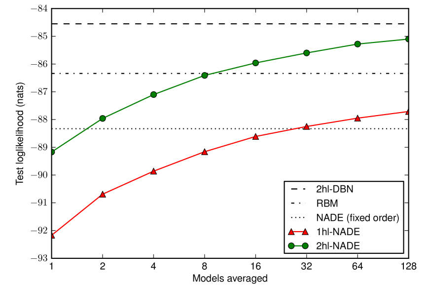
Ensembles of NADEs obtained by using NADEs with different variable orderings but trained simultaneously with our order-agnostic procedure obtain better statistical performance than NADEs trained using a fixed ordering. These EoNADEs can also surpass the estimated performance of RBMs with the same number of hidden units, and even approach the estimated performance of a (larger) 2-hidden-layer deep belief network. A more detailed account of the statistical performance of EoNADEs can be seen in Figure 1. We also report the performance on NADE trained by minimizing $\mathcal{J}_{\scriptscriptstyle OA}$ but without input masks. Input masks are necessary for obtaining competitive results.

Table 2: Average test-set log-likelihood per datapoint of different models on $28\!\times\!28$ binarized images of digits taken from MNIST.

Model	Test LogL
MoBernoullis K=10	$-168.95$
MoBernoullis K=500	$-137.64$
RBM (500 h, 25 CD steps) approx.	$-86.34$
DBN 2hl approx.	$\mathbf{-84.55}$
NADE 1hl (fixed order)	$-88.86$
NADE 1hl (fixed order, RLU, minibatch)	$-88.33$
NADE 1hl (fixed order, sigm, minibatch)	$-88.35$
NADE 1hl (no input masks)	$-99.37$
NADE 2hl (no input masks)	$-95.33$
NADE 1hl	$-92.17$
NADE 2hl	$-89.17$
NADE 3hl	$-89.38$
NADE 4hl	$-89.60$
EoNADE 1hl (2 orderings)	$-90.69$
EoNADE 1hl (128 orderings)	$-87.71$
EoNADE 2hl (2 orderings)	$-87.96$
EoNADE 2hl (128 orderings)	$-85.10$

Figure 1: Test-set average log-likelihood per datapoint for RNADEs trained with our new procedure on binarized images of digits.

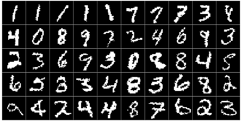
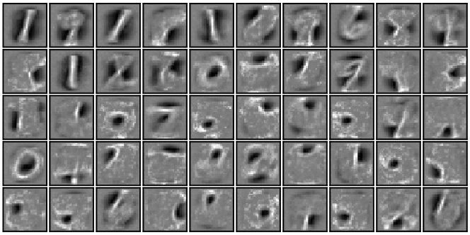
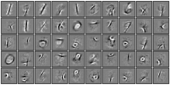
Samples from a 2 hidden layer (500 hidden units per layer) NADE trained using the order-agnostic method are shown in Figure 2. Most of the samples can be identified as digits. Figure 4 shows some receptive fields from the model’s first hidden layer (i.e. columns of $\boldsymbol{W}$). Most of the receptive fields resemble pen strokes. We also show their associated receptive fields on the input masks . These can be thought of as biases that activate or deactivate a hidden unit. Most of them will activate the unit when the input mask contains a region of unknown values (zeros in the input mask) flanked by a region of known values (ones in the input mask).

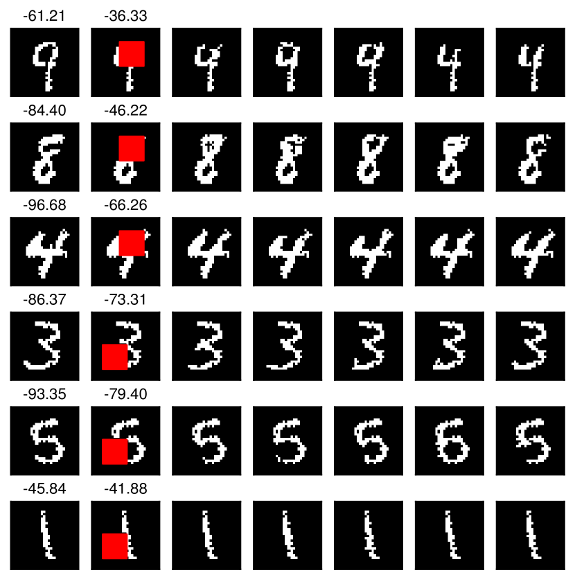
Having at our disposal a NADE for each possible ordering of the inputs makes it easy to perform any inference task. In Figure 3 we show examples of marginalization and imputation tasks. Arbitrarily chosen regions of digits in the MNIST test-set are to be marginalized or sampled from. An RBM or a DBN would require an exponential number of operations to calculate either the marginal density or the density of the complete images. A NADE trained on a fixed ordering of the variables would be able to easily calculate the densities of the complete images, but would require approximate inference to calculate the marginal densities. Both an RBM and a fixed-order NADE require MCMC methods in order to sample the hollowed regions. However, with our order-agnostic training procedure we can easily calculate the marginal densities and sample the hollowed regions in constant time just by constructing a NADE with a convenient ordering of the pixels.

Figure 2: Top: 50 examples from binarized-MNIST ordered by decreasing likelihood under a 2-hidden-layer NADE. Bottom:  50 samples from a 2-hidden-layer NADE, also ordered by decreasing likelihood under the model.

Figure 3: Example of marginalization and sampling. First column shows five examples from the test set of the MNIST dataset. The second column shows the density of these examples when a random 10 by 10 pixel region is marginalized. The right-most five columns show samples for the hollowed region. Both tasks can be done easily with a NADE where the pixels to marginalize are at the end of the ordering.

Figure 4: Top:50 receptive fields (columns of $\boldsymbol{W}$) with the biggest L2 norm. Bottom: Associated receptive fields to the input masks.

6.2 Real-valued datasets

We also compared the performance of RNADEs trained with our order-agnostic procedure to RNADEs trained for a fixed ordering. We start by comparing the performance on three low-dimensional UCI datasets (Bache & Lichman, 2013) of heterogeneous data, namely: red wine, white wine and parkinsons. We dropped the other two datasets tested by Uria et al. (2013), because some of their dimensions only take a finite number of values even if those are real-valued. We report the test-log-likelihood on 10 folds of the dataset, each with 90% of the data used for training and 10% for testing. All experiments use normalized data. Each dimension is normalized separately by subtracting its training-set average and dividing by its standard deviation.

Experimental details follow. Learning rate and weight decay rates were chosen by per-fold cross-validation; using grid search. One ninth of the training set examples were used for validation purposes. Once the hyperparameter values had been chosen, a final experiment was run using all the training data. In order to prevent overfitting, training was stopped when observing a training likelihood higher than the one obtained at the optimal stopping point in the corresponding validation run. All RNADEs trained had a mixture of 20 Gaussian components for output, and were trained by stochastic gradient descent on $\mathcal{J}_{\scriptscriptstyle OA}$. We fixed the number of hidden units to 50, following Uria et al. (2013). The learning rate was chosen among $\{0.02,0.005,0.002,0.0005\}$ and the weight decay rate among $\{0.02,0.002,0\}$.

The results are shown in Table 3. RNADEs trained using our procedure obtain results close to those of RNADEs trained for a fixed ordering on the red wine and white wine datasets. On the Parkinsons dataset, RNADEs trained for a fixed ordering perform better. Ensembles of RNADEs obtained better statistical performance on the three datasets.

Table 3: Average test log-likelihood for different models on three real-valued UCI datasets. Baselines are taken from (Uria et al., 2013).

Model	Red wine	White wine	Parkinsons
Gaussian	$-13.18$	$-13.20$	$-10.85$
MFA	$-10.19$	$-10.73$	$-1.99$
RNADE (fixed)	$\mathbf{-9.36}$	$\mathbf{-10.23}$	$\mathbf{-0.90}$
RNADE 1hl	$-9.49$	$-10.35$	$-2.67$
RNADE 2hl	$-9.63$	$\mathbf{-10.23}$	$-2.19$
RNADE 3hl	$-9.54$	$\mathbf{-10.21}$	$-2.13$
RNADE 1hl 2 ord.	$-9.07$	$-10.03$	$-1.97$
RNADE 2hl 2 ord.	$-9.13$	$-9.84$	$-1.42$
RNADE 3hl 2 ord.	$-8.93$	$-9.79$	$-1.39$
RNADE 1hl 16 ord.	$-8.95$	$-9.94$	$-1.73$
RNADE 2hl 16 ord.	$-8.98$	$-9.69$	$-1.16$
RNADE 3hl 16 ord.	$\mathbf{-8.76}$	$\mathbf{-9.67}$	$-1.13$

We also measured the performance of our new training procedure on 8 by 8 patches of natural images in the BSDS300 dataset. We compare the performance of RNADEs with different number of hidden layers trained with our procedure against a one-hidden layer RNADE trained for a fixed ordering (Uria et al., 2013), and with mixtures of Gaussians, which remain the state of the art in this problem (Zoran & Weiss, 2012).

We adopted the setup described by Uria et al. (2013). The average intensity of each patch was subtracted from each pixel’s value. After this, all datapoints lay on a 63-dimensional subspace, for this reason only 63 pixels were modelled, discarding the bottom-right pixel.

Experimental details follow. The dataset’s 200 training image set was partitioned into a training set and a validation set of 180 and 20 images respectively. Hyperparameters were chosen by preliminary manual search on the model likelihood for the validation dataset. We used a mixture of 10 Gaussian components for the output distribution of each pixel. All hidden layers were fixed to a size of 1000 units. The minibatch size was set to 1000. Training was run for 2000 iterations, each consisting of 1000 weight updates. The initial learning rate was set to 0.001. Pretraining of hidden layers was done for 50 iterations.

The results are shown in Table 4. RNADEs with less than 3 hidden layers trained using our order-agnostic procedure obtained lower statistical performance than a fixed-ordering NADE and a mixture of Gaussians. However RNADEs with more than 3 layers are able to beat both baselines and obtain what are, to the extent of our knowledge, the best results ever reported on this task. Ensembles of RNADEs also show an improvement in statistical performance compared to the use of single RNADEs.

No signs of overfitting were observed. Even when using 6 hidden layers, the cost on the validation dataset never started increasing steadily during training. Therefore it may be possible to obtain even better results using more hidden layers or more hidden units per layer.

Table 4: Average test-set log-likelihood for several models trained on 8 by 8 pixel patches of natural images taken from the BSDS300 dataset. Note that because these are log probability densities they are positive, higher is better.

Model	Test LogL
MoG $K\!=\!200$ (Zoran & Weiss, 2012)	$152.8$
RNADE 1hl (fixed order)	$152.1$
RNADE 1hl	$143.2$
RNADE 2hl	$149.2$
RNADE 3hl	$152.0$
RNADE 4hl	$153.6$
RNADE 5hl	$154.7$
RNADE 6hl	$\mathbf{155.2}$
EoRNADE 6hl 2 ord.	$156.0$
EoRNADE 6hl 32 ord.	$\mathbf{157.0}$

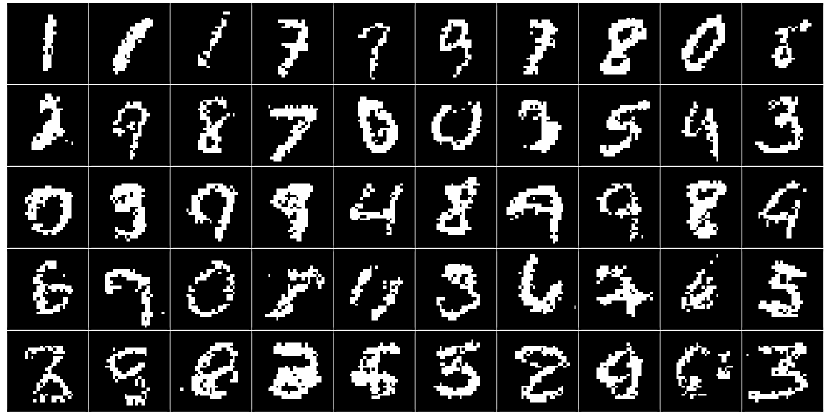
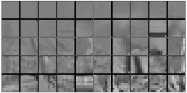
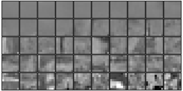
Samples from the 6 hidden layers NADE trained in an order-agnostic manner are shown in Figure 5.

Figure 5: Top: 50 examples of $8\!\times\!8$ patches in the BSDS300 dataset ordered by decreasing likelihood under a 6-hidden-layer NADE. Bottom:  50 samples from a 6-hidden-layer NADE.

7 Conclusions

We have introduced a new training procedure that simultaneously fits a NADE for each possible ordering of the dimensions. In addition, this new training procedure is able to train deep versions of NADE with a linear increase in computation, and construct ensembles of NADEs on the fly without incurring any extra training computational cost.

NADEs trained with our procedure outperform mixture models in all datasets we have investigated. However, for most datasets several hidden layers are required to surpass or equal the performance of NADEs trained for a fixed ordering of the variables. Nonetheless, our method allows fast and exact marginalization and sampling, unlike the rest of the methods compared.

Models trained using our order-agnostic procedure obtained what are, to the best of our knowledge, the best statistical performances ever reported on the BSDS300 8$\times$8-image-patches datasets. The use of ensembles of NADEs, which we can obtain at no extra training cost and have a mild effect on test-time cost, improved statistical performance on most datasets analyzed.

Acknowledgments

We thank John Bridle and Steve Renals for useful discussions.

References

- Bache & Lichman (2013) Bache, K. and Lichman, M. UCI machine learning repository, 2013. http://archive.ics.uci.edu/ml.
- Bengio (2009) Bengio, Y. Learning deep architectures for AI. Foundations and trends in Machine Learning, 2(1):1–127, 2009.
- Bengio & Bengio (2000) Bengio, Y. and Bengio, S. Modeling high-dimensional discrete data with multi-layer neural networks. In Advances in Neural Information Processing Systems 12 (NIPS 1999), pp. 400–406. MIT Press, 2000.
- Bishop (1994) Bishop, C. M. Mixture density networks. Technical report, Neural Computing Research Group, Aston University, 1994.
- Bishop (2006) Bishop, C. M. Pattern recognition and machine learning. Springer–Verlag, New York, 2006. ISBN 0387310738.
- Frey (1998) Frey, B. J. Graphical models for machine learning and digital communication. MIT Press, 1998.
- Goodfellow et al. (2013) Goodfellow, I., Mirza, M., Courville, A., and Bengio, Y. Multi-prediction deep Boltzmann machines. In Advances in Neural Information Processing Systems 26, pp. 548–556. 2013.
- Gregor & LeCun (2011) Gregor, K. and LeCun, Y. Learning representations by maximizing compression. Technical report, arXiv:1108.1169, 2011.
- Larochelle & Murray (2011) Larochelle, H. and Murray, I. The Neural Autoregressive Distribution Estimator. In Proceedings of the 14th International Conference on Artificial Intelligence and Statistics (AISTATS 2011), volume 15, pp. 29–37, Ft. Lauderdale, USA, 2011. JMLR W&CP.
- Murray & Salakhutdinov (2009) Murray, I. and Salakhutdinov, R. Evaluating probabilities under high-dimensional latent variable models. In Advances in Neural Information Processing Systems 21 (NIPS 2008), pp. 1137–1144, 2009.
- Nair & Hinton (2010) Nair, V. and Hinton, G. E. Rectified linear units improve restricted Boltzmann machines. In Proceedings of the 27th International Conference on Machine Learning (ICML-10), pp. 807–814, 2010.
- Ormoneit & Tresp (1996) Ormoneit, D. and Tresp, V. Improved Gaussian mixture density estimates using Bayesian penalty terms and network averaging. In Advances in Neural Information Processing Systems 8 (NIPS 1995), pp. 542–548. MIT Press, 1996.
- Salakhutdinov & Murray (2008) Salakhutdinov, R. and Murray, I. On the quantitative analysis of deep belief networks. In Proceedings of the 25th International Conference on Machine Learning (ICML 2008), volume 25, pp. 872–879, 2008.
- Smyth & Wolpert (1999) Smyth, P. and Wolpert, D. Linearly combining density estimators via stacking. Machine Learning, 36(1-2):59–83, 1999.
- Sutskever (2013) Sutskever, I. Training recurrent neural networks. PhD thesis, University of Toronto, 2013.
- Uria et al. (2013) Uria, B., Murray, I., and Larochelle, H. RNADE: The real-valued neural autoregressive density-estimator. In Advances in Neural Information Processing Systems 26 (NIPS 26), 2013. To appear. arXiv:1306.0186.
- Vincent et al. (2008) Vincent, P., Larochelle, H., Bengio, Y., and Manzagol, P. A. Extracting and composing robust features with denoising autoencoders. In Proceedings of the 25th International Conference on Machine Learning (ICML 2008), pp. 1096–1103, Helsinki, Finland, 2008. ACM.
- Zoran & Weiss (2012) Zoran, D. and Weiss, Y. Natural images, Gaussian mixtures and dead leaves. In Advances in Neural Information Processing Systems 25 (NIPS 2012), pp. 1745–1753, 2012.