Random spanning forests,
Markov matrix spectra and well distributed points
Abstract
This paper is a variation on the uniform spanning tree theme. We use random spanning forests to solve the following problem: for a Markov process on a finite set of size , find a probability law on the subsets of any given size with the property that the mean hitting time of such a random target does not depend on the starting point of the random walk. We then explore the connection between random spanning forests and infinitesimal generator spectrum. In particular we give an almost probabilistic proof of an algebraic result due to Micchelli and Willoughby [18] and used by Fill [8] and Miclo [19] to study the convergence to equilibrium of reversible Markov chains. We finally introduce some related fragmentation and coalescence processes, emphasizing algorithmic aspects, and give an extension of Burton and Pemantle transfer current theorem [2] to the non reversible case.
MSC 2010: primary: 05C81,60J20,15A15; secondary: 15A18,05C85.
Keywords: Finite networks, spectral analysis,
spanning forests, determinantal processes, transfer current theorem,
random sets, hitting times, local equilibria,
Wilson’s algorithm, random partitions, coalescence and fragmentation.
1 A random set problem and a forest measure
1.1 “Well distributed points” in a given graph
Let us consider the following problem. We have a square chessboard with sides of length and a simple random walk on it. More precisely, think the chessboard as the square lattice box with the simple random walk on . Denote by the hitting time of a set for the walk and by the law of starting from . Can you find a probability law on the subsets of with cardinality such that
| (1.1) |
In other words, can you sample “well distributed points” among the points of ? In this example, a possible simple answer is the following: take to be the set of either white or black squares of the chessboard with probability .
One could then raise the following questions:
-
•
What if the random subsets are required to have any other cardinality ?
-
•
What if, instead of the chessboard , we consider any other finite weighted, possibly oriented, graph?
We notice that the case is trivial, and that in the case , it is known that it suffices to choose the point in according to the stationary measure of the walk (see e.g. Lemma 10.8 in [16]). One of the main goal of this paper is to answer these questions for .
In the sequel, we work on a finite oriented weighted graph with its naturally associated continuous time Markov process. We study a certain probability measure on the set of spanning rooted oriented forests on this graph. It will turn out that the set of roots of the forest sampled from this measure, with conditioning on the number of roots, provides a solution to our random set problem in full generality. As far as practical sampling issues are concerned, by using an algorithm due to Wilson and Propp [23, 20] we can sample this measure without conditioning. Furthermore, under the assumption that the generator of the random walk associated with the starting weighted graph has only real eigenvalues, we explain how to get a sample with an approximate prescribed number of roots within an error of order . In Section 1.2 below, we introduce the main framework and notation, and in Section 1.3 we describe the structure of the paper and the results we derive.
1.2 Forest measures
Let be a Markov process on a finite state space , with . Assume is irreducible with generator given by
| (1.2) |
with arbitrary and a given collection of non-negative transition rates. Note that such a Markov process has variable speed depending on the current state, namely, if the chain is at position , the next jump will be performed after an exponential time of rate
| (1.3) |
The collections of rates induces a structure of oriented weighted graph on . In fact, consider the set of oriented edges
| (1.4) |
then is a weighted oriented graph.
The main object of our investigation is a measure on the spanning rooted forests of . These are the oriented subgraphs of that can be described in the following way. Call an -spanning unrooted forest any simple undirected graph without cycle and with as set of vertices. The connected components of such a graph are trees. By specifying a root, that is a particular vertex, in each of these trees, we can define an oriented graph by orienting the edges of each rooted tree towards its root. If is a subgraph of , i.e., if each (oriented) edge of belongs to , we call it a spanning rooted forest of . We will identify with the collection of its edges, that is with a subset of , and we call the set of the spanning rooted forests of . In particular is the spanning forest made of degenerated trees reduced to simple roots. For we define the weight of a such a forest
| (1.5) |
Definition 1.1.
(Standard forest measure) Denote by the set of roots of a forest . Fix and define on the measure given by
| (1.6) |
By normalizing it via the partition function
| (1.7) |
we denote the resulting probability measure by
| (1.8) |
We call standard measure, standard partition function and standard probability measure, the objects defined by equations (1.6), (1.7), and (1.8), respectively.
Remarks: In the case of symmetric rates , there are obvious similarities between the weights appearing in equation (1.6) and those of Fortuyn-Kasteleyn model. We stress here the main differences. FK-percolation is defined on spanning graphs that are not required to be forests. However, in the zero limit of its main parameters, properly rescaled, the model does converge to a measure on spanning forests (see e.g. [11]). Nevertheless, our forests are rooted and this extra structure introduces an entropic factor in comparison (by projection on unrooted forests) with this zero limit of FK-percolation. To make it precise, let us call the set of unrooted spanning forests of , with obtained from by identifying each edge with it ‘opposite’ . To each rooted forest is associated, by construction, a unique unrooted forest . On the one hand, the weight associated in (the zero limit of) FK-percolation to each is proportional to
| (1.9) |
where is the set of the connected component of , i.e., the set of all maximal trees contained in . On the other hand, if is a random forest with law , then, for each ,
| (1.10) |
with the set of vertices spanned by the tree (by seeing as a set of edges, one has ). There are indeed, ways of choosing roots for the trees of . We get by projection a cluster size biased version of the zero limit of FK-percolation.
We also note that the weights in (1.5) are those associated by Freidlin and Wentzell with the so called “-graphs” [9] and we will recover some of their results in this paper. Our standard forest measure has also been studied in various works. For example to sample points from the stationary measure of the random walk [20], or to study in [13] recurrent configurations of Abelian dissipative sandpile introduced in [22]. This spanning forest measure and other associated objects we will discuss later are actually a variation on the theme of uniform spanning trees and loop-erased random walks. We refer to [15] and references therein for the vast literature on the subject.
As it will become clear, the measure in Definition 1.1 and the associated partition function encode several information related to the chain . At the occurrence, we will derive results related with slightly more general measures and partition functions. To this aim, we introduce here some further notation. Let us first introduce a natural generalization of the measure in Definition 1.1. Given a collection of extra weights , let be the diagonal matrix defined by for (and when ). We anticipate that these extra weights will be interpreted as killing rates for the chain . Set
| (1.11) |
and define the measure by
| (1.12) |
By assuming that there is at least one with we can turn into a probability measure on by normalizing it via the partition function:
| (1.13) |
and we denote the resulting probability measure by
| (1.14) |
This is the general form of the probability measure at the core of our investigation.
When answering the questions raised in Section 1.1, we need the following special case of the generalized measure in (1.12). For a given subset , suppose that the collection of extra weights is such that
| (1.15) |
In this case, and we write
| (1.16) |
for the associated measure, partition function and probability, , and , respectively. In particular, for and , and . Note further that, when (and ), we recover the standard measure and partition function, and .
In the sequel we will denote by a random variable on a probability space with values in and law . We will also write and in the corresponding special cases.
1.3 Results and structure of the paper
1.3.1 Main results
Our analysis of the forest measures introduced above will lead us to several results. Before describing them and the organization of the paper, we emphasize herein what we consider as our four main results.
Determinantal roots: First, in Theorem 3.4 we prove that the set of roots is a determinantal process. In particular, denoting by
| (1.17) |
the transition probabilities of the Markov chain in (1.2) observed at independent exponentially distributed times of parameter , we show that
| (1.18) |
with being the determinant of restricted to (see Section 1.3.3 below for the notation). This echoes Burton and Pemantle transfer current theorem ([2], Theorem 1.1). on spanning trees associated with reversible Markov processes. Our generator and our kernel are however not required to be reversible (and they possibly have complex eigenvalues) and we present a direct proof not relying on transfer currents. We will actually later use our random rooted forests to prove transfer current theorems for random rooted and unrooted spanning trees associated with non-reversible Markov processes.
Random target: The second result is an answer to the questions in the introductory Section 1.1. In fact, in Theorem 4.1 we give a formula for the hitting times of random sets constituted by the roots of our standard random forests, with or without conditioning on having a fixed number of roots. In particular, such a formula is independent of the starting point . While Wilson and Propp algorithm gives a way to sample the unconditioned measure, in Section 4 we explain how to obtain, in absence of complex eigenvalues, a sample with approximately roots, with an error of order , for any .
Local equilibria: Our third result concerns the proof on an algebraic statement on symmetric matrices derived by Micchelli and Willoughby [18], Theorem 3.2 therein. This theorem has been used in [8, 19] to study absorption times of reversible Markov chains on general finite graphs, as a key tool to define, in such a general setting, the local equilibria introduced in [6]. In [19] the author motivates the importance of having a probabilistic interpretation of Micchelli and Willoughby algebraic result. In Section 5 we restate their result and give, by means of our standard forest measure, a probabilistic presentation of their proof.
Transfer current: These three main results focus on the root process or and show its deep connection with the spectrum of . In Section 7 we start instead, like in [3], from the study of the whole edge process of the spanning forest to give in Theorem 7.2 an extension of transfer current theorems for spanning trees to the non reversible case. This is our last main result.
1.3.2 Organization of the paper
The rest of the paper is organized as follows.
Background material: Section 2 is a warm-up section where we provide some known background material. In Section 2.1 we prove in a slightly different way a result originally due to Marchal [17] on loop-erased trajectories (Proposition 2.1). In Section 2.2 we recall Wilson’s algorithm (Definition 2.2) and, following [17, 20], we show how to sample our unconditioned measures (Corollary 2.3).
Results: Section 3 presents the first analysis on our forest measure, mainly focusing on the root process. In Theorem 3.1 and Corollary 3.2 therein we show some connection of this measures with the spectrum of the chain . We prove that the set of roots is a determinantal process (Theorem 3.4) and compute its cumulants, or truncated correlation functions (Lemma 3.5). In Section 4 we prove Theorem 4.1 on the hitting times of the root set, answering the questions raised in Section 1.1. We also compute the mean return time in the set of roots for the Markov process started from a uniformly chosen root (Theorem 4.2) and estimate the expected value of the largest mean hitting time of the root set (Theorem 4.3). Section 5 presents Micchelli and Willoughby [18] result and proof in a probabilistic way. In Section 6 we mention two coalescence and fragmentation processes associated with our measures. One of them give some information on the “rooted partition” induced by our spanning forests (Proposition 6.4). The other one is obtained by coupling together all the standard forest measures for different values of and raises a number of open questions. In Section 7 we study the full edge process to extend classical transfer current theorems in Theorem 7.2.
Appendix: Four appendix sections are devoted to known results used along the paper and that we derive in our context in order to have a self-contained work. In Appendix A, we recall what is the Schur complement for block matrices and its probabilistic interpretation (Proposition A.1). In Appendix B, we give different proofs of two lemmas from Freidlin and Wentzell (Lemmas 3.2, 3.3 in [9]) on hitting distribution and times of subsets of the graph, again by analysing of our forest measure. This is used in Section 4. Appendix C concerns the notion of divided differences which are used in Section 5. We state three equivalent definitions and prove a related lemma. In Appendix D we write in our context the proof of Theorem 7.1, which is due to Chang [3] and which we use in Section 7.
To conclude this introductory section and to simplify the reading, we fix here some notation. Further notation will be introduced at the occurrence.
1.3.3 Main notation
- Sets
-
- Spaces:
-
will be our reference state space of size for the irreducible Markov process . In the sequel, we work with extensions of which will be denoted by or with more general spaces denoted by .
- Subsets:
-
the symbols and will be used as inclusion and strict inclusion, respectively. Subsets will be generally denoted by capital letters: .
- Complement:
-
the complement of a set will be denoted by , and it will be clear from the context, with respect to which set is this complement defined.
- Graphs
-
- Edges:
-
introduced in (1.4) stands for the set of oriented edges on . For , is its associated weight.
- Extreme points of oriented edges:
-
for an oriented edge , we denote the starting and the ending points of and by and .
- Reversed edges:
-
for an oriented edge , stands for its ‘opposite’ .
- Forest space:
-
denotes the set of spanning rooted oriented forests on .
- A given forest:
-
elements of are denoted by and are identified with subsets of .
- Roots:
-
given , denotes the set of the roots of the trees in .
- Tree associated with a given vertex:
-
given in and we denote by the unique maximal tree in that covers . We write when is rooted at .
- Matrices
-
- Identity:
-
for we denote by the identity matrix and we identify with the identity operator on the space of functions . We also write for .
- Restriction of a matrix:
-
given a matrix , for any subset of , stands for the restriction of to its elements that are doubly indexed in : .
- Determinants:
-
will denote the determinant of the matrix obtained from by removing all the lines and columns with indexes outside , i.e., .
- Characteristic polynomial:
-
we will often write instead of for the characteristic polynomial of .
- Markov processes
-
- Continuous time processes and discrete time random walks:
-
and will denote Markov processes on the finite spaces and , respectively. and will denote some associated discrete-time Markov chains, which generally are not obtained from and by taking the sequence of positions of and at their successive jumps from a position in and to a distinct one.
- Generators:
-
and denote the generators of the Markov processes and respectively. For a given subset of , , and respectively stand for the Markovian or sub-Markovian generators of the process restricted to , the process killed outside and the trace of on respectively. In other words, if the action of on functions is defined by
(1.19) then is the Markovian generator of a process on and acts on functions according to
(1.20) is the sub-Markovian generator obtained from the matrix representation of by deleting the row and columns with indices outside and acts on functions according to
(1.21) and is the Schur complement of in , which defines another Markov process on (see Appendix A for more details).
2 Background material
2.1 On loop-erased trajectories
We introduce here a slightly more general setting than in Section 1.2. Let be a Markov process on a finite state space with a generator given by
| (2.1) |
with arbitrary and a given collection of non-negative transition rates (to avoid ambiguities, we assume that for each in there is at most one such that ). Let
| (2.2) |
Let be a subset of such that
| (2.3) |
so that, for any , the complement of in . We assume that is accessible from any starting point of the process .
Denote by a self-avoiding path of points and length such that for and . For , let the law of the random walk when starting from . Denote by a random trajectory obtained from under as follows: stop the walk when it enters the set for the first time and erase all its loops. After this procedure, we are left with a self-avoiding trajectory of variable length. In the next proposition we compute the probability that is the given trajectory . To this end, we use a discrete skeleton of the Markov process absorbed in . This justify the following definitions.
Set
| (2.4) |
and let be the stochastic matrix, with , identified by the entries
| (2.5) |
Such a matrix is a Markovian transition matrix for a discrete-time random walk on . In particular, for an arbitrary function , by construction we have that
| (2.6) |
We are in shape to prove the claimed proposition, by using a nice independence argument we learned from Laurent Tournier.
Proposition 2.1.
Proof.
For the discrete chain , let and be the first return time to and the hitting time of , respectively. More precisely, and . Note that by definition of we have
| (2.8) |
As a consequence, we can write:
| (2.9) | ||||
It follows from (2.9) that
| (2.10) |
Denote by the local time spends at before entering , and by the matrix restricted to , then
| (2.11) | ||||
where the last equality follows by Cramer’s formula for an inverse matrix.
On the other hand, for the numerator in the r.h.s. of equation (2.10), we can write
| (2.12) |
2.2 Wilson’s algorithm
We introduce here the algorithm due to Wilson and Propp [20] which allow us to sample the measure (1.14). First, we extend the Markov process defined through (1.2) on to a Markov process on the space by interpreting as an absorbing state and by adding some killing rates. Consider the space , with . Assume a collection of killing rates is given, and let be the diagonal matrix with diagonal entries , . Consider the Markov process on the finite state space with generator given by
| (2.14) |
with arbitrary, and defined in (1.2). In particular, the matrix associated with the generator in (2.14) satisfies
| (2.15) |
Next, we describe the algorithm. For any , note that, due to irreducibility, is a.s. finite.
Definition 2.2.
(Wilson’s algorithm)
-
1.
Start the process from any point until it reaches the absorbing state .
-
2.
Erase all the loops of the trajectory described by up to time . Call this self-avoiding trajectory. ( is such that is the last point in .)
-
3.
If covers the whole stop, else pick any point , with denoting the set of points covered by . Start the process from until it hits the set .
-
4.
Erase all the loops of the trajectory described by starting from up to time . Call this self-avoiding trajectory.
-
5.
If stop, else pick any point . Start the process from until it hits the set .
-
6.
Iterate until is covered.
Denote by the set of spanning oriented trees on rooted at . This algorithm produces in finite time an element of . As a corollary of Proposition 2.1, we can easily compute the probability that the algorithm produces a given .
Corollary 2.3.
Fix a tree . Let be the set of edges in that point to the root . Denote by the probability that Wilson’s algorithm produces the tree . Then
| (2.16) |
with .
Proof.
Recall the notation in Proposition 2.1. Set and . Start with . By the definition of the algorithm, the proof follows by iterating the formula in equation (2.7) where at each iteration we set the right according to the given tree . Whatever the choice of starting points in Wilson’s algorithm we get the same result. ∎
We conclude this section by observing that there exists a natural bijection between and . Indeed, given , let be the unique element in obtained from by adding all the edges connecting the roots in to , i.e. add all edges such that and . Vice versa, given , by removing all edges we can identify a unique element . This simple observation together with Corollary 2.3 allow us to sample the measure in (1.14) using Wilson’s algorithm.
3 The root process
3.1 Partition function and root number distribution
We start here to analyze the measure introduced in (1.14) on the space of spanning rooted oriented forests on . We compute the partition function, we identify the distribution of the number of roots in the standard case and we prove that the root process is a determinantal one.
Theorem 3.1.
(Partition function and spectrum) Assume a collection of killing rates is given, and let be the diagonal matrix with diagonal entries , . Let the probability measure on in (1.14). Then
| (3.1) |
and, recalling the notation from Section 2.2,
| (3.2) |
In the case , we recover the standard probability measure in (1.8), and the standard partition function in (1.7) is given by the characteristic polynomial of
| (3.3) |
where the ’s are the eigenvalues of ordered by non-decreasing real part. When and , the partition function is given by the characteristic polynomial of the sub-Markovian generator of the process killed in :
| (3.4) |
Remark: This kind of results goes back to Kirchhoff [14]. Here, like in [4], Theorem 3’, we include the non-reversible case and stress the dependence in .
Proof.
In the standard case, an immediate consequence of Theorem 3.1 is a characterization of the law of the cardinality of the set of roots.
Corollary 3.2.
(Root number distribution) Assume the standard case and that has real spectrum. Let be a sum of independent Bernoulli random variables with parameters . The random variable counting the number of roots (or equivalently, of trees) in has the same law as .
Proof.
Observe that the coefficient of degree in
| (3.7) |
is the total weight of the set of forest with exactly roots. Since we get,
| (3.8) | ||||
where stands for the set of all possible elements of the set . ∎
Remark: When the spectrum of does contain a non-real part, one can still compute the law of and get the same algebraic expressions in terms of the eigenvalues. One can also compute momenta by differentiating with respect to the logarithm of the partition function. In particular, the mean value and the variance are given by
| (3.9) | |||
| (3.10) |
We note however that the contribution of the imaginary part of the eigenvalues can make uneasy the comparison between variance and mean value, at least for small values of . This is the reason why, when dealing with the question of getting samples with a number of roots that approximates a given , we will restrict ourselves to the real spectrum case.
3.2 Determinantal structure
Next, we prove that the random set , or more generally , is a determinantal process as suggested after [7] by the previous result. This is the content of Theorem 3.4 for which we will present an algebraic and a probabilistic proof.
Let us first show a simple lemma. Consider the Markov process on defined via its generator in (2.14). This process can be coupled up to time with a Markov process in which is stopped at rate in any . Calling this stopping time, is then the last point visited in by the process before time , or, in other words, the end point of the last egde crossed inside , before going directly to .
Let be the Markovian matrix defined by
| (3.11) |
This transition kernel can also be expressed in terms of the Green’s function :
Lemma 3.3.
Proof.
Note that, when or , we have
| (3.15) |
with being an independent exponential random variable of parameter . In particular, if is the Green’s function up to time , then
| (3.16) |
Theorem 3.4.
(Determinantal roots) The root process is a determinantal process with kernel . Equivalently, for any :
| (3.17) |
Proof.
(Algebraic proof of Thm 3.4) Assume first . Consider a set with of the form . By choosing the different points in as starting point at each iteration in Wilson’s algorithm (remember that the law of the obtained tree does not depend on the order of the starting points), by (2.7), we get
| (3.18) | ||||
In case , the claim is straightforward since equation (3.18) reads
| (3.19) |
and the r.h.s. equals due to Lemma 3.3.
Proof.
(Probabilistic proof of Thm 3.4) To avoid a heavy notation, we consider only the case . Starting from the Markov process and the killing rates , we construct two different absorbing states and accessible from the set and , respectively. Set . Let be the Markov process with generator
| (3.23) | ||||
and if with and as in (1.2).
Next, consider the subspace . Let be the Markov process with state space obtained as the trace of the process on . Let us remark two features of Wilson’s algorithm. First, Wilson’s algorithm can be extended to the case of a state space with more than one absorbing state. In this case it produces a rooted spanning forest instead of a tree. Second, Wilson’s algorithm is uniquely determined once we fix a state space with some absorbing set and a Markov generator. These observations justify the following definitions. Let be the set of ending points of the edges starting from after running Wilson algorithm on with absorbing state and generator . Similarly let associated in the same way with , when Wilson’s algorithm is run on with absorbing set and generator . Observe at this point that
| (3.24) |
and, by using Proposition 2.1, compute
| (3.25) | ||||
where denotes the Green’s function of the process stopped when entering the absorbing states . Note now that for ,
| (3.26) |
with and being the Green’s function of the process in (2.14). Finally, since for , the claim follows by combining equations (3.25) and (3.26). ∎
3.3 Cumulants
In this section we compute the cumulants of the determinantal process : they are given by a nice formula it is worth to notice. Let us associate with our random forests with law , the random variables
| (3.27) |
note that they completely describe the root process. For with distinct ’s, the cumulants of these random variables are defined by
| (3.28) |
These quantities are the so-called truncated correlation functions, that can also be recursively defined by
| (3.29) |
where stands for the set of partitions of .
The determinantal nature of the root process makes its cumulants easy to compute. With and being the permutation group on , one has
| (3.30) |
Making a cycle decomposition of each permutation in this sum and denoting by the set of long cycles on , i.e. the set of cycles of length in , after some simple algebra, we get
| (3.31) |
This identifies our cumulants through (3.29) and gives the following lemma.
Lemma 3.5.
For all
| (3.32) |
where stands for the set of cycles of length in .
Remark: In the case of uniformly equal weights between nearest neighbours, for large , behaves like the natural low temperature partition function associated with an embedded travelling salesman problem. In this regime, on the one hand, Wilson’s algorithm quickly provides perfect samples of the root process and, on the other hand, the cumulant is the expected value of some observable for the system made of independent copies of [21]. This suggests that one could find a practical way to estimate this low temperature partition function and then solve the travelling salesman problem. Unfortunately, the corresponding observable has an exponentially small probability to be different from and consequently, it is in reality impossible to estimate its mean in this way.
4 Hitting times
In this section we answer the question raised in the introductory Section 1.1. To this end, we focus on hitting times of a given subset , i.e.,
| (4.1) |
We will also look at the return time
| (4.2) |
The reason why we use this heavy double + notation is that we will also consider the often more useful randomized or skeleton return time , which is defined as follows. Assume that is built from a discrete time skeleton such that is updated according to the successive positions of after independent exponential times of parameter
| (4.3) |
so that, with the transition matrix of ,
| (4.4) |
The randomized or skeleton return time is
| (4.5) |
with the first updating time (which is an exponential time of parameter ). One always has and, for , it holds
| (4.6) |
so that
| (4.7) |
with as in (1.3).
In Appendix B, Lemma B.1, we prove, with the help of Wilson’s algorithm and elementary Green’s function computations, a formula for , which is originally due to Freidlin and Wentzell (Lemma 3.3 in [9]). We will use this formula to compute the mean value of when is the set of roots sampled from either or for any given .
Theorem 4.1.
(Hitting-time formulas) For any
| (4.8) |
with being the unique tree in containing . In the standard case, , equation (4.8) reduces to
| (4.9) |
Moreover, for and any ,
| (4.10) |
with the coefficient of degree in the characteristic polynomial
| (4.11) |
Proof.
Note that the r.h.s. of (4.9) and (4.10) is independent of the starting point . This latter observation allows to answer the questions in the introduction. In fact, no matter the geometry of the graph and the weights we are considering, we can take the random subset of which is given by the root set of a random forest with law , and the formula in equation (4.10) says that the hitting times do not dependent on the starting point .
To practically obtain a sample from with approximately roots when has only real eigenvalues, one can use Wilson’s algorithm and play with the parameter as follows. If is such that
| (4.14) |
one has an expected number of roots with fluctuations of order or smaller (see Corollary 3.2). In principle one should compute the eigenvalues of , which is in general difficult for large , and then solve equation (4.14) in . To overcome this obstacle, a possible alternative procedure is the following:
-
1.
Start with any positive and run Wilson’s algorithm with this parameter to get a sample from with a certain number of roots.
-
2.
Replace by and run again Wilson’s algorithm with this new parameter to get a new sample with another number of roots, say again.
-
3.
Iterate the previous step until a sample with roots satisfying is obtained.
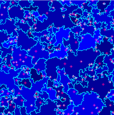
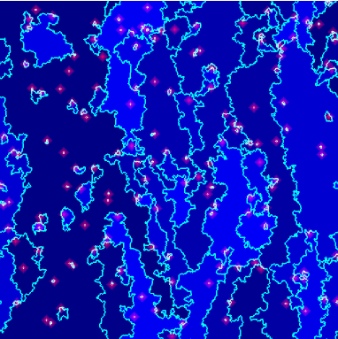
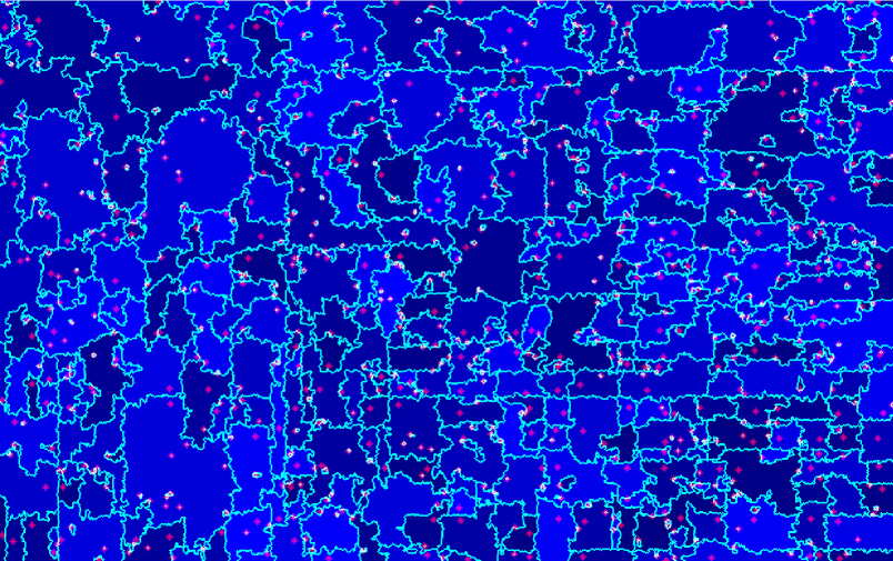
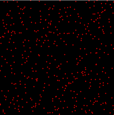
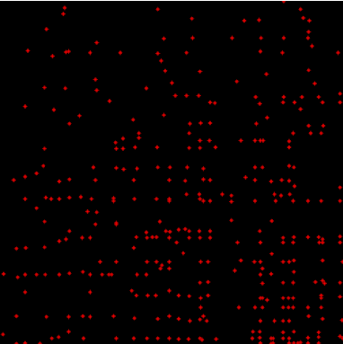
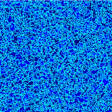
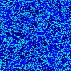
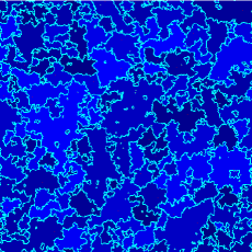
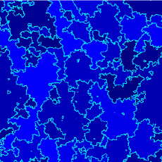
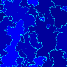
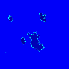
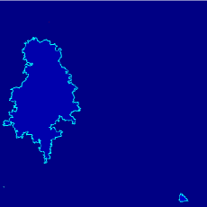
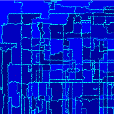
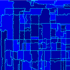
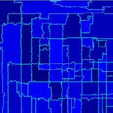
As a matter of fact, rapidly converges to the solution of (4.14), hence the algorithm rapidly reaches an end. Since we believe this procedure to be quite far from an optimal one, we are only sketchy on this point. Jus to give some example, we sampled in this way approximatively 100000, 10000, 1000 and 100 roots on the grid for the random walk in a Brownian sheet potential with inverse temperature . We obtained 100443, 10032, 1042 and 111 roots in 8, 6, 6 and 8 iterations, respectively.
In equation (4.9) and (4.10) the starting point is given and does not depend on the root set . The next two propositions deal with the mean value of (recall (4.2)-(1.3)) when is uniformly chosen in and with the mean value of .
Proposition 4.2.
(Return-time in ) For all in , all and all positive , it holds
| (4.15) |
and
| (4.16) |
In particular,
| (4.17) |
and
| (4.18) |
where stands for a random point uniformly distributed in .
Proof.
Along this proof, for an arbitrary subset , we write for either or and we set for any in . If , then , while, when ,
| (4.19) |
Setting , we also have, when ,
| (4.20) |
By defining for all in X, we then get
| (4.21) | ||||
where in the last equality we have used that if , and that since is a probability measure on subsets of . Now Theorem 4.1 says that the function is constant on , therefore harmonic on . Equivalently, for any , which together with (4.21) implies that
| (4.22) |
By recalling the definition of and passing in continuous time, we see that equation (4.22) is equivalent to (4.15). Equation (4.16) is then a consequence of (4.7).
Proposition 4.3.
(Largest expected hitting-time estimates) For all it holds
| (4.24) |
Furthermore, for any positive , it holds (recall the notation of Theorem 4.1)
| (4.25) |
Proof.
As we remarked before, Wilson’s algorithm works also when considering more than one absorbing state. Denote by the running time of Wilson’s algorithm (i.e. the total running time of the loop erased random walks needed to cover the whole graph) when the absorbing states form a non-empty subset of (this amounts to sample ). It can be shown (see e.g. [17], Proposition 1) that the mean running time111 This running time is actually independent of the obtained sample and its law is the same as that of a sum of independent exponential variables with parameters when these eigenvalues are real. The same holds in the case of complex eigenvalues by defining “the sum of exponential variables” through its Laplace transform and the same algebraic formula as in the real case. can be expressed in spectral terms as , with being the eigenvalues of the operator , the sub-Markovian generator associated with the process absorbed in . Note at this point that we can overestimate the l.h.s. of (4.24) by the expectation of . Hence, using (3.4) and looking at the coefficient of degree 1 in ,
| (4.26) | ||||
and the latter equals the r.h.s. of (4.24). The bounds in (4.25) follows by a similar argument. ∎
Remark: These estimates can often be a gross overestimation of the largest expected hitting time as soon as is not very small or very large, or when is not close to or . It is not difficult however to build examples for which the estimates are tight for all and . (One can for example consider a one dimensional random walk with drift.)
5 Re-reading Micchelli-Willoughby proof
Throughout this section we work with the Markov process on in (1.2), under the assumption that is reversible with respect to some probability measure on , i.e., is a self-adjoint operator in endowed with the inner product
| (5.1) |
For , possibly , we turn the points of into “absorbing points” by adding infinite weight edges towards a cemetery . We denote by , with , the eigenvalues of , and following [6, 8, 19], we define, for each in , a sequence of local equilibria by setting
| (5.2) | |||||
| (5.3) |
Theorem 3.2 in [18] is a statement on symmetric matrices that in our setting can be described as follows.
Theorem 5.1.
(Micchelli and Willoughby [18]) For all in and all , is a non-negative measure.
In this section we give a proof of this theorem following the key steps of Micchelli and Willoughby’s algebraic proof, however, unlike the original proof, we develop probabilistic or combinatorial arguments.
Before starting the proof we note, following [19], that equation (5.3) can be rewritten as
| (5.4) |
which gives the following interpretation. The process leaves the measure, or “state”, at rate to be absorbed in or to decay into . This can be turned into a rigorous mathematical statement [17], provided that and are indeed non-negative measures, as claimed in Theorem 5.1. Then, by looking at the different decay times up to an exponential time that is independent from the process, and by observing that, by Hamilton-Cayley theorem, the process leaves the state at rate only to be absorbed in , we get, for all and in ,
| (5.5) |
The left hand side in (5.5) is the probability to have . Then, multiplying by (recall (3.4)), dividing by , and denoting the result by , we have on the right hand side
| (5.6) |
or, equivalently,
| (5.7) |
while equation (5.5) now reads
| (5.8) |
Next, in order to prove Theorem 5.1, we can restrict ourselves, by density and continuity, to the case of distinct eigenvalues. Then equation (5.8) suggests, for , the following relation for the divided differences (see Definition C.3 in Appendix C) of :
| (5.9) |
that is
| (5.10) |
It is worth to stress at this point we have just seen that equation (5.10) would be a consequence of Theorem 5.1, but our goal is to prove Theorem 5.1. This is what we are ready to do now by following the main steps of Micchelli and Willoughby’s proof.
Step 1: Checking equation (5.10) (without assuming Theorem 5.1…).
We simply use Definition C.3 and spectral decomposition.
With being the right eigenvector associated with ,
and, for any measure , ,
we have for any and with defined by (5.6),
| (5.11) |
This gives
| (5.12) | ||||
and, by arbitrariness of , equation (5.10) readily follows.
Step 2: A combinatorial identity.
The key point of the proof lies in the following lemma.
Lemma 5.2.
For any in ,
| (5.13) |
In addition one has
| (5.14) |
Proof.
Let us first consider the case . Due to (5.7), we have that
| (5.15) |
We also have
| (5.16) |
and
| (5.17) |
Next, define for each in (5.15), if belongs to , and if is connected in to through and (possibly with ) in such a way that and belong to . Finally, by observing that and , (5.13) is obtained from (5.15), (5.16) and (5.17). Then, equation (5.14) follows from (5.15) for . ∎
Step 3: Conclusion by induction with Cauchy interlacement theorem.
For , let be the following statement:
For all such that , for all , for all such that for all , for all , and for all :
We can proceed inductively to show that holds.
For , the claim is obvious. Fix . In the case , the inductive hypothesis is unnecessary. Indeed, from (5.14), one has
| (5.18) |
Then note that, by Cauchy interlacement theorem, implies that for , and hence, by Lemma C.4, we get
| (5.19) |
When , follows in the same way by using (5.13) and the inductive hypothesis.
6 Rooted partitions, coalescence and fragmentation
In this section we present two coalescence and fragmentation processes closely related with our forest measures. The first one is obtain by coupling together all our forest measures . The second one admits as invariant measure and gives some information on the “rooted partition” which is naturally associated with each spanning rooted forest.
6.1 Coupling the forest measures for different values of .
The coupling we present can be seen as a coalescence and fragmentation process when decreases to and is thought as time. The main idea is to make use of Wilson’s original representation of his algorithm with “site-indexed random paths” which we present in the next two paragraphs.
6.1.1 Random walk: stack representation
Assume that, to each site of the graph, is attached an infinite list or collection of arrows pointing towards one neighbour, and that these arrows are independently distributed according to the discrete skeleton transition probabilities as defined by equations (4.3)-(4.4). In other words, an arrow, pointing towards the neighbour of a site , appears at each level in the list associated with with probability (in this context, we set , and consider itself as one of its possible neighbours). Imagine that each list of arrows attached to a site is piled down in such a way that it make sense to talk of an infinite stack with an arrow on the top of this stack. By using this representation, one can generate the random walk on the graph as follows. At each jump time, the random walk steps to the neighbour pointed by the arrow on the top of the stack where the walker is sitting, and the top arrow is erased from the stack. This representation is often referred to as the Diaconis-Fulton representation (see [5]).
6.1.2 Wilson’s algorithm: stack representation
To describe Wilson’s algorithm one has to introduce a further ingredient: pointers to the absorbing state in each stack. Such a pointer should appear with probability at each level in the stack. One way to introduce it is by generating independent uniform random variables together with each original arrow in the stack, and by replacing the latter by a pointer to the absorbing state whenever .
A possible description of Wilson’s algorithm is then the following.
-
i.
Start with a particle on each site. Both particles and sites will be declared either active or frozen. At the beginning all sites and particles are declared to be active.
-
ii.
Choose an arbitrary particle among all the active ones and look at the arrow at the top of the stack it is seated on. Call the site where the particle is seated.
-
–
If the arrow is the pointer towards , declare the particle to be frozen and site as well.
-
–
If the arrow points towards another site , remove the particle and keep the arrow. We say that this arrow is now uncovered.
-
–
If the arrow points to itself, remove the arrow.
-
–
-
iii.
Once again, choose an arbitrary particle among all the active ones, look at the arrow on the top of the stack it is seated on, and call the site where the particle is seated.
-
–
If the arrow points to , the particle is declared to be frozen, and so are declared and all the sites eventually leading to by following uncovered top pile arrow paths.
-
–
If the arrow points to a frozen site, remove the chosen particle at , keep the (now uncovered) arrow, and freeze site as well as any site eventually leading to by following uncovered top pile arrow paths.
-
–
If the arrow points to an active site, then there are two possibilities. By following the uncovered arrows at the top of the stacks, we either reach a different active particle, or run in a loop back to . In the former case, remove the chosen particle from site and keep the discovered arrow. In the latter, erase all the arrows along the loop and put an active particle on each site of the loop. Note that this last case includes the possibility for the discovered arrow of pointing to itself, in which case, we just have to remove the discovered arrow.
-
–
-
iv.
Iterate the previous step up to exhaustion of the active particles.
The crucial observation is that, no matter of the choice of the particles at the beginning of the steps, when this algorithm stops, the same arrows are erased and the same spanning forest of uncovered arrows and with a frozen particle at each root is obtained. In particular, by choosing at each step the last encountered active particle, or the same as in the previous step when we just erased a loop, we perform a simple loop-erased random walk up to freezing.
6.1.3 Coupling and sampling
Since can be sampled using Wilson’s algorithm as described above, and the same uniform variables can be used for each , this provides a coupling among all the ’s. By means of this coupling, one can actually sample starting from a sample of for . Let us now explain this fact. Note first that, running this algorithm for sampling , one can reach at some point the final configuration obtained for with the only difference that some frozen particles of the final configuration obtained with parameter can still be active at this intermediate step of the algorithm run with . It suffices, indeed, to choose the sequence of active particles in the same way with both parameters. This is possible since each pointer to in the stacks with parameter is associated with a pointer to at the same level in the stacks with parameter . Thus, to obtain a sample of from a sample of , we just have to replace some frozen particle of the configuration sampled with and continue the algorithm with parameter . To decide which particle in has to be unfrozen or not we can proceed as follows. With probability
| (6.1) |
each particle in , independently from each other, is kept frozen. With probability a particle in a site in is declared active, is also declared active and we set at the top of the pile in an arrow that points toward with probability .
6.1.4 Coalescence and fragmentation process: trajectories
When continuously decreases, we obtain a coalescence-fragmentation process in which each tree can fragment and partially coalesce with the other trees of the forest. When a root of a tree turns active, the tree is eventually fragmented into a forest, some trees of which being possibly “grafted" on the previous frozen trees. It is worth noting that, by (3.9), the mean number of trees is decreasing along this coalescence-fragmentation process.
The previous observations show that we can sample the “finite dimensional distributions” of the process, i.e. the law of for any choice of . We can actually sample whole trajectories for any finite . In fact, note first that at each time , the next frozen particle (or root) becoming active is uniformly distributed among all the roots, and the time when it “wakes up" is such that the variable
| (6.2) |
has the law of the maximum of independent uniform variables on , with being the number of roots at time . Since, for all ,
| (6.3) |
has the same law as , with uniform on . Using (6.2) we can then sample by setting
| (6.4) |
Summing up, in order to sample the whole trajectory it suffices to proceed as follows once is sampled at a given jump time :
-
•
Choose uniformly a root in .
-
•
Sample the next jump time from a uniform random variable on , by using (6.4).
-
•
Restart the algorithm with parameter by declaring active the particle in and putting an arrow to with probability .
The next proposition characterizes the law of the process .
Proposition 6.1.
If for all , then, for any and any ,
| (6.5) |
with for all , and .
Proof.
We first prove (6.5) in the case , when . The observations made in Section 6.1.3 imply that as far as the event is concerned, conditioning on is nothing but conditioning on the value of the uniform random variables at the top of the stacks in . Using the previous terminology, if we keep ‘frozen’ each site in with probability defined in (6.1) and we call the set of the remaining frozen sites, will not be a determinantal process with kernel . Indeed, the waking up procedure we described after (6.1) implies a bias on the distribution of the top pile arrow at the unfrozen sites: such an arrow cannot be replaced by a pointer to . To recover a determinantal process with kernel , the set has to be built by keeping frozen each site in with a smaller probability solving
| (6.6) |
In such a way the top pile arrow at each unfrozen site can still be replaced by a pointer to with probability , and (6.6) implies that we recover the correct biased probability. Solving (6.6) gives and (6.5) follows.
When is larger than 1, the formula is simply obtained by keeping frozen each site in with a probability that depends on the largest such that . This is the reason why the sets are introduced: is the largest such that , if and only if . ∎


We conclude this section with some open questions.
-
1.
It is a fact that “crosses" almost surely all the manifolds
(6.7) Indeed, by (3.9), it starts from and reaches almost surely, and, each time the number of roots decreases, it does so by only 1 unit: when the “activated" tree fragments into trees that coalesce only with the previously frozen ones. With
(6.8) it is also simple to sample . But the measure is not the law of . Is there however a way to use that process to sample this measure?
-
2.
One can use that process to estimate for all large enough , since this is the expected root number of . Is it then possible to use it to estimate the spectrum of , or at least the higher part of it in an efficient way ?
-
3.
Is it possible to characterize the law of the rooted partition process associated with like we described the law of ? This partition is the one for which two sites and lie in the same component at time when they are covered by the same tree in with . It is ‘rooted’ since a special point, the root of the tree, is associated with each component of the partition. We know very little on the law of this partition for each given (see next section). An easier question would be that of describing the forest process itself, since we know that can be described as a determinantal process for each (see Section 7).
6.2 Rooted partition and the forest measure as invariant measure of another coalescence and fragmentation process
The other dynamics we want to mention is a simple variant of the tree random walk introduced in [1] to prove the so called Markov chain tree theorem. For fixed , the dynamics we now present is another coalescence and fragmentation process for which the standard measure is the stationary probability measure.
Remind that for a given forest and , we denote by the unique tree in containing , and note that if then . Our dynamics can then be defined as follows.
Definition 6.2.
(Forest Dynamics) Fix . Let be the Markov process with state space characterized by the following formula for the generator acting on functions :
| (6.9) |
where the transition rate and the new state are defined as follows:
-
1.
If and , then and .
-
2.
If and , then and , with being the unique edge in such that .
-
3.
If , then and .
-
4.
else.
The rules corresponding to 1, 2 and 3 can be rephrased by saying that we add, swap and remove a bond from the forest , respectively. Notice that such a dynamics induces a non-conservative dynamics on the set of roots. In particular, when transition 1 occurs, and two trees merge into one. On the other hand, when transition 3 occurs, and the tree containing is fragmented into two trees where the new appearing root is at . Transitions of type 2 produce a rearranging in one of the tree. They leave invariant the cardinality of the set of roots but the location of the root in the modified tree is relocated at the vertex .
Proposition 6.3.
Proof.
We have to show that for any
| (6.10) |
For a given , we start by splitting the l.h.s. of (6.10) in the three terms corresponding to the different transitions allowed by the dynamics in Definition 6.2 whenever .
| (6.11) | ||||
We can rewrite
| (6.12) |
| (6.13) |
and, denoting, for each such that and , by the unique bond in the only one cycle of such that , with ,
| (6.14) |
Summing , and together we then get (6.10). ∎
Remark: When we recover the Anantharam and Tsoukas dynamics and the proof of the Markov tree theorem. Indeed, the standard forest measure restricted to spanning trees is the invariant measure of the dynamics. Starting with a single tree, its roots follows a Markovian evolution with generator , so that, at equilibrium, in the long time limit we have
| (6.15) |
with being the stationary distribution associated to .
We can then describe the position of the roots given the “tree partition” associated with . For in with roots , …, , let us denote by the partition of where each component is the set of sites spanned by . Since each piece of the partition comes with a special point corresponding to a root, we call rooted partition the pair We note that for each in , the restricted dynamics with generator
| (6.16) |
has only one irreducible component since each in is connected with the root. As a consequence the restricted dynamics has a unique equilibrium measure which we call restricted measure . Note that when has a reversible equilibrium , then is nothing but the equilibrium measure conditioned on , i.e. .
Proposition 6.4.
(Roots in restricted equilibrium) Fix , then
| (6.17) |
for any partition of and any , for
Proof.
For each in , let us call the set of rooted spanning trees of . For each in , define
| (6.18) |
and for in , write , if is the root of the tree . Compute
| (6.19) | ||||
where the last equality follows by (6.15) applied to the restricted dynamics. ∎
Remark: When is reversible with respect to a measure , this gives a way to build the associated Gaussian free field with mass , that is the Gaussian process with covariance matrix
| (6.20) |
by successive sampling of the standard measure . Start from independent centered random variables with variance , , sample according to , call the set of vertices of and set
| (6.21) |
Then the random field has zero mean and covariance matrix and the rescaled partial sums , with , , …independent copies of , converges in law to as goes to infinity. Indeed, for each and in , and are centered and one computes
| (6.22) |
Since, following Wilson’s algorithm,
| (6.23) | ||||
| (6.24) | ||||
| (6.25) |
we conclude
| (6.26) |
7 The edge process
We assume in this section that is a non-zero collection of finite killing rates. The infinite rate case can simply be obtained by computing the corresponding limit in the next assertions.
The next theorem is due to Chang [3]. We write it with our notation and in Appendix D we give Chang’s proof in our context for completion. Let us first introduce some more notation. Given on and in we call
| (7.1) |
the expected number of crossings of the (oriented) edge up to time . We also define the net flow through starting from by
| (7.2) |
Theorem 7.1.
(Chang [3]) For any
| (7.3) |
with
| (7.4) |
In addition, denoting by the event that for all either or belong to , it holds
| (7.5) |
with
| (7.6) |
Remark: In the symmetric case for all , by choosing for all one obtains, as a consequence of (7.5), a proof of a tree-size biased version of the negative edge correlation conjecture for the uniform unrooted spanning forest (see [12, 10]). Recalling (1.10), one has indeed, for each and in and the associated unoriented edges and in ,
| (7.7) |
where the square in the first equation is a consequence of the reversibility of the Green’s kernel with respect to the uniform measure. But we were unable to deduce from this a proof of the original conjecture.
Consider the random forest for a given and killing matrix . Set and notice that, as goes to 0, converges in law to a random spanning tree with distribution
| (7.8) |
where stands for the root of the spanning tree . By (6.15) this is the law of a random tree obtained by running Wilson’s algorithm with root choosen with probability
| (7.9) |
and used as the absorbing state. Chang [3] showed that is also a determinantal process. By computing the same limits in a different way, we give here a different proof and, more importantly, a different expression for the kernel, allowing for an easy comparison with the reversible transfer current theorem. For in and in we define as the expected number of crossings of the (oriented) edge by the process started from and stopped at the hitting time of , . We also define the net flow through by
| (7.10) |
Theorem 7.2.
(Transfer current theorem) For any
| (7.11) |
with
| (7.12) |
where
| (7.13) |
In addition,
| (7.14) |
with
| (7.15) |
Remark: In the reversible case one has, for any in and in , , so that
| (7.16) |
and we recover Burton and Pemantle’s theorem [2]. The difference
| (7.17) |
is indeed the net flow through the edge during the commutation between and , i.e, along the process started from and stopped at its first return to after . Since, by reversibility, each such path appears in the corresponding expectation with the same weight as its reversed path, and it contributes to the net flow with the opposite sign, the difference (7.17) is equal to zero.
Proof.
We simply compute the limit of as goes to 0. To this end we set and, for any , we denote by the (random) number of crossing of the edge (from to ) in the time interval . Hence and
| (7.18) |
Set , , define recursively
| (7.19) |
and notice that
| (7.20) |
With
| (7.21) |
and
| (7.22) |
we get
| (7.23) |
and
| (7.24) |
By differentiating in equation (7.21) one gets
| (7.25) |
and
| (7.26) |
Appendix A Schur complement and trace process
Assume we have a Markov process on a finite state space , with generator given by
| (A.1) |
with arbitrary and a given collection of non-negative and finite transition rates. With
| (A.2) |
we define a discrete skeleton of with transition matrix such that
| (A.3) |
In other words, can be build from by updating the position of the process after independant exponential times of paramater according to the position sequence of .
Fix a subset and define a new Markov chain with state space obtained as the trace of the process on . In other words, is the random walk with transition matrix with entries
| (A.4) |
where denotes the first return time in of the chain .
Back to the continuous-time setting, denote by be the continuous-time version of with jump times given by exponential random variables of parameter
| (A.5) |
i.e. the process with generator
| (A.6) |
Equivalently, is the trace of the Markov process on , namely, the process obtained by following the trajectory of at infinite velocity outside and without speeding up inside .
Proposition A.1.
(Schur complement and trace process) Given the Markov process on with generator , fix a subset . Let be the generator of the Markov process obtained as the trace of the process on . Then, is the Schur complement of in , i.e.
| (A.7) |
where and are the operators obtained from the matrix representation of , by keeping only those rates from to and to , respectively.
Proof.
Denote by , the sub-Markovian matrix restricted to . Note that is different from . Due to (A.4), for any , we can write
| (A.8) | ||||
Subtracting on both side of (A.8), we obtain that
| (A.9) |
We then get our result by multiplying both sides by . ∎
When contains an absorbing set and we can do the same computation with the sub-Markovian generator in place of . For any and in the mean local time in starting from and before hitting is the same for and the trace process , i.e.
| (A.10) |
that is
| (A.11) |
or, to be more concise, . More generally, one has the following definition and properties.
Definition A.2.
(Schur complement) Let be an matrix written as block matrix
| (A.12) |
where , , and for some . The Schur complement of in is defined as the matrix
| (A.13) |
Appendix B Lemma on hitting distributions and times
In this section we use our forest measure analysis to prove two formulas on the hitting distribution and the expectation of hitting times of a given subset of the given graph. This result is originally due to Freidlin and Wentzell, see Lemmas 3.2 and 3.3 in [9].
Lemma B.1.
Proof.
Consider the extended space and the extended Markov process as in (2.14), with the killing rates as in (1.15) for . Equation (B.1) is simply obtained by considering Wilson’s algorithm started from .
To prove (B.2) we will use the discrete skeleton of the absorbed process of Section (2.1) with and . Let
| (B.3) |
be the continuous and the discrete time Green’s functions before hitting the set , respectively.
Since , it suffices to show that, for all ,
| (B.4) |
Since with being the return time to ,
| (B.5) | ||||
Observe that for any , thus using (B.1):
| (B.6) | ||||
∎
Appendix C Divided differences
In this appendix, we recall three equivalent definitions of the notion of divided differences of a real function. We further give a lemma due to Micchelli and Willoughby for which we provide an alternative elementary proof which plays with these different definitions. This result is used in Section 5.
Definition C.1.
(Divided differences 1) We call divided difference of a function at the distinct points , , …, , the quantity recursively defined via
| (C.1) |
with
| (C.2) |
From this definition, we see that the divided differences at points of a function can be seen as a sort of -th discrete derivative. One then show by induction
Definition C.2.
(Divided differences 2) For any function and distinct points , , …, , ,
| (C.3) |
Note in this second definition, that is independent of the order of the ’s. From (C.3) one can then check
Definition C.3.
(Divided differences 3) For any function and distinct points , , …, , ,
| (C.4) | ||||
is the unique polynomial of degree with , for
Lemma C.4.
(Micchelli and Willoughby [18]) Consider a polynomial of degree of the form
| (C.5) |
with distinct real zeros in decreasing order: . Let with and such that
| (C.6) |
Then, for any ,
| (C.7) |
Proof.
We prove the following statement by induction on :
| “For any satisfying (C.6), .” | (C.8) |
Since is a polynomial of degree , (C.8) follows from Definition C.4 as soon as . Also, since the dominant coefficient of is , the same argument shows and the claim holds for . Fix now , i.e. , and satisfying (C.6). If then
| (C.9) | ||||
| (C.10) | ||||
| (C.11) |
By Definition C.3 we have and the numerator in the l.h.s. of (C.9) is merely equal to . The denominator is positive from (C.6) and so is the r.h.s. of (C.11) by induction hypothesis. It follows that
| (C.12) |
and the same is true when . If , we compute
| (C.13) |
get then in the same way
| (C.14) |
and the same is true when . Proceeding similarly we eventually obtain that
| (C.15) |
∎
Appendix D Proof of Theorem 7.1
To prove (7.3) we first note that the left-hand side is equal to zero as soon as there are two distinct edges and in such that , and so is the right-hand side, since one gets two proportional columns in the corresponding restricted matrix. We then assume that for each in
| (D.1) |
there is a unique in such that . Let us compute
| (D.2) |
By Theorem 3.1 and the sum appearing in (D.2) is equal to , with the Markovian generator obtain from by setting to zero all rates such that and with , and with obtained from just by setting to zero all the rates for in .
This gives
| (D.3) |
and we can compute row by row this matrix product. Observing that, for each , has to be the diagonal term in each line of the matrix representation of , we obtain
| (D.4) |
We then get (7.3) by using the bloc triangular structure of this product and redistributing the terms of the product in the computed determinant.
To prove (7.5) we introduce the matrices
| (D.5) |
observe that, for all and in ,
| (D.6) |
and note that
| (D.7) |
is the coefficient of degree in the polynomial in
| (D.8) |
where is the identity matrix. Elementary operations on rows and columns give then
| (D.9) |
The coefficient of degree in this polynomial in is then
| (D.10) |
Acknowledgements: A.G. thanks Laurent Tournier for the many fruitful discussions on the matter, and, in particular, the nice independence argument we presented in Section 2. He also thanks Pablo Ferrari, Inès Armendariz, Pablo Groisman, Leonardo Rolla and Matthieu Jonckheere for their hospitality at Buenos Aires where all this work started. L.A. has been supported by DFG SPP Priority Programme 1590 Probabilistic Structures in Evolution and by NWO Gravitation Grant 024.002.003-NETWORKS.
References
- [1] V. Anantharam and P. Tsoucas, A proof of the Markov chain tree theorem, Statist. Probab. Lett., 8(2), 189–192 (1989).
- [2] R. Burton and R. Pemantle, Local characteristics, entropy and limit theorems for spanning trees and domino tilings via transfer-impedances, Ann. Probab. 21, 1329–1371 (1993).
- [3] Y. Chang, Contribution à l’étude des lacets markoviens. Université Paris Sud - Paris XI (2013) <tel-00846462>
- [4] P. Chebotarev and R. Agaev, Forest matrices around the Laplacian matrix, Linear Algebra and its Applications, 356(1–3), 253–274 (2002).
- [5] P. Diaconis and W. Fulton. A growth model, a game, an algebra, Lagrange inversion, and characteristic classes. Rend. Sem. Mat. Univ. Pol. Torino, 49(1), 95–119 (1991).
- [6] P. Diaconis and L. Miclo, On times to quasi-stationarity for birth and death processes, J. Theoret. Probab. 22(3), 558–586 (2009).
- [7] J. B. Hough, M. Krishnapur, Y. Peres and B. Virag, Determinantal processes and independence, Probab. Surv. 3, 206–229 (2006).
- [8] J. Fill, On hitting times and fastest strong stationary times for skip-free and more general chains, J. Theor. Probab. 22, 587–600 (2009).
- [9] M. I. Freidlin and A. D. Wentzell, Random perturbations of dynamical systems, Grundlehren der Mathematischen Wissenschaften 260, (Second edition ed.). New York: Springer-Verlag (1998).
- [10] G. R. Grimmet and S. N. Winkler, Negative association in uniform forests and connected graphs, Random Structures Algorithms 24, 444–460 (2004).
- [11] G. R. Grimmett, The random-cluster model, Grundlehren der mathematischen Wissenschaften 333, Springer (2006).
- [12] J. Kahn, A normal law for matchings, Combinatorica 20(3), 339–391 (2000)
- [13] A. A. Járai, F. Redig and E. Saada, Zero dissipation limit in the Abelian sandpile model, Preprint: arXiv:0906.3128v3 (2011).
- [14] G. Kirchhoff, Über di Auflösung der Gleichungen, auf welche man bei der Untersuchung der linearen Verteilung galvnischer Ströme geführt wird, Ann. Phys. chem 72, 497–508 (1847).
- [15] Y. Le Jan, Markov paths, loops and fields, vol. 2026 of Lecture Notes in Mathematics. Springer, Heidelberg, 2011. Lectures from the 38th Probability Summer School held in Saint-Flour, 2008, Ecole d’Été de Probabilités de Saint-Flour.
- [16] D. A. Levin, Y. Peres and E. L. Wilmer, Markov chains and mixing times, American Mathematical Society (2008).
- [17] P. Marchal, Loop-erased random walks, spanning trees and Hamiltonian cycles, Elect. Comm. Probab. 5 , 39–50 (2000).
- [18] C. A. Micchelli and R. A. Willoughby, On functions which preserve the class of Stieltjes matrices, Lin. Alg. Appl. 23, 141–156 (1979).
- [19] L. Miclo, On absorption times and Dirichlet eigenvalues, ESAIM: Probability and Statistics 14, 117–150 (2010).
- [20] J. Propp and D. Wilson, How to get a perfectly random sample from a generic Markov chain and generate a random spanning tree of a directed graph, Journal of Algorithms 27, 170–217 (1998).
- [21] G. S. Sylvester, Representations and inequalities for Ising model Ursell functions, Comm. Math. Phys. 42, 209–220 (1975).
- [22] V. T. Tsuchiya and M. Katori, Proof of breaking of self-organized criticality in a nonconservative abelian sandpile model, Phys. Rev. E 61, 1183–1188 (2000).
- [23] D. Wilson, Generating random spanning trees more quickly than the cover time, Proceedings of the twenty-eighth annual acm symposium on the theory of computing, 296–303 (1996).