Dynamically generated darkness in the Dicke model

Abstract

We study the dynamics of a driven Dicke model, where the collective spin is rotated with a constant velocity around a fixed axis. The time evolution of the mean photon number and of the atomic inversion is calculated using, on the one hand, a numerical technique for the quantum dynamics of a small number of two-level atoms, on the other hand, time-dependent mean-field theory for the limit of a large number of atoms. We observe a reduction of the mean photon number as compared to its equilibrium value. This dynamically generated darkness is particularly pronounced slightly above the transition to a superradiant phase. We attribute the effect to a slowing down of the motion in the classical limit of a large ensemble and to an interplay of dynamic and geometric phases in the quantum case.

I Introduction

The Dicke model Dicke1954 , TC describes $N$ two-level atoms interacting with a single-mode radiation field through the dipole coupling. If the atoms are confined to a region of space which is much smaller than the wavelength of the radiation field, the two-level emitters behave as a single large spin. The model is a paradigm for the collective behavior of matter interacting with light. In the thermodynamic limit, $N\rightarrow\infty$, there is a transition to a superradiant phase at a critical coupling strength HL , WH , CGW . The order parameter can be chosen to be the photon density, which vanishes in the normal phase and is finite in the superradiant phase. Alternatively one may also use the fraction of excited atoms, which behaves similarly to the photon density. Recently the emphasis was on the quantum phase transition at zero temperature. It could be shown that the entanglement between photons and atoms diverges by approaching the quantum-critical point Lambert . Interestingly, for finite $N$ clear signatures of the onset of quantum chaos are also found for couplings at and not too far above the quantum-critical point Emary2003 .

The existence of this phase transition in a real material was called seriously into question some time ago. It was argued that adding the term proportional to $A^{2}$ to the Dicke model, where $A$ is the vector potential of the electromagnetic field, would eliminate the equilibrium transition RWZ . However, in a more recent study it was pointed out that within a consistent treatment of interactions between excited atoms a transition would still occur, although maybe of a different type than originally thought Keeling , VD . A different route would be to realize the Dicke model in a non-equilibrium setting of cavity quantum electrodynamics Dimer . An experimental breakthrough was achieved with a high-quality cavity hosting a Bose-Einstein condensate Esslinger . This setup is not only considered to be a realization of the Dicke model, it also produced data showing evidence for a superradiant phase transition and other collective behaviors Esslinger_2 .

The combination of cold atomic gases and cavity quantum electrodynamics has the advantage that parameter values can be tuned with high precision and even controlled in real time. This type of experiments has stimulated studies of non-equilibrium effects and, especially, their interplay with collective phenomena, for instance in the vicinity of a quantum phase transition. A fundamental problem is the evolution of an initial state – or density matrix – in a model without dissipation. For the (time-independent) Dicke model an approach to equilibrium has been found, governed by a competition between classical chaos and quantum diffusion AH . The Dicke model turns into a many-body Landau-Zener model if both atomic and photonic excitation energies become time-dependent. In contrast to the usual Landau-Zener model with a single two-level system, where an adiabatic evolution - and thus no tunneling - is easily achieved for slow enough driving, this becomes very difficult in the problem involving many two-level systems AGKP . At the critical point an adiabatic evolution appears to be impossible IT . A different scenario is obtained if the coupling constant is time-dependent. Here a rich new phase diagram including metastable phases and first-order transitions has been reported BERB .

In several papers dealing with the dynamics of the Dicke model the rotating wave approximation has been used, where the emission of a photon is accompanied by the transition of an excited atom to its ground state and the absorption of a photon is linked to the excitation of an atom. This yields an integrable model where the dynamics is not chaotic. In one study the evolution after an initial quench has been found to lead either to a constant photon density at long times or to produce persistent oscillations with several incommensurable frequencies Yuzbashyan . Other studies investigated the conditions under which a classical treatment of the dynamics is valid TL , Faribault .

In this paper we consider a specific time-dependent coupling where the spin operator is rotated with a time-dependent angle. This “rotated Dicke Hamiltonian” can be generated by a unitary transformation starting from the time-independent Hamiltonian. Therefore the energy eigenvalues do not depend on time, in contrast to the study mentioned above BERB . Nevertheless the evolution is highly nontrivial and leads to qualitatively new effects at and slightly above the equilibrium quantum critical point. We are particularly interested in the thermodynamic limit, where a time-dependent mean-field theory is expected to yield exact results for the dynamics. We develop this theory on the basis of a coherent state representation of both photon and spin degrees of freedom. We obtain a classical dynamical system of two oscillators, which are coupled by a nonlinear time-dependent term. Alternatively, this classical limit can also be reached in the framework of the Holstein-Primakoff transformation. Once the classical dynamical system is established, it is straightforward to calculate the relevant physical quantities, such as the (time-dependent) photon density. For finite $N$ we complement the mean-field calculations by a numerical procedure where the quantum evolution for a specific initial state is computed for the rotated Dicke Hamiltonian. For large $N$, these numerical results approach the mean-field predictions, as expected.

In our calculations we kept all coupling terms of the Dicke model and did not use the rotating wave approximation. At weak coupling one does not find noticeable effects of the terms neglected by the rotating wave approximation, but at and above the quantum critical point the differences between integrable and non-integrable cases show up clearly, for instance through the onset of chaos in the latter case.

The following general picture emerges from our calculations. The rotation by a time-dependent angle leads to an upshift of the critical coupling strength above which a finite photon density is produced spontaneously. If the system is prepared in the ground state of the (time-independent) Dicke model slightly above its quantum-critical point, i.e. with a finite photon density, an interesting darkening effect occurs after the rotation is switched on. A clear minimum in the photon density is found as a function of the coupling strength for a fixed driving velocity or, even more pronounced, as a function of driving velocity for a fixed coupling strength. The location of the minimum defines a dynamical critical line in the coupling versus velocity plane. The effect can be readily understood as a slowing down of the nonlinear dynamics in the classical limit. For a small number of two-level systems, where the evolution has to be treated quantum mechanically, we find that the geometric phase associated with the time-dependent state of the system plays a crucial role in this dynamically generated darkness.

The paper is organized as follows. Section II gives a short review of the standard (time-independent) Dicke model. The time-dependent Dicke model is introduced in Section III. The rotation by a time-dependent angle can be partly compensated by a transformation to a co-rotating frame. The numerical procedure used for treating the quantum dynamics of a limited number of two-level systems is also explained. Section IV presents the time-dependent mean-field theory using coherent states for both the spin and the photons. The stationary states in the co-rotating frame yields a modified phase diagram, as compared to that of the time-independent Dicke model. Two linear modes describe motions close to equilibrium, one of which softens by approaching criticality. However, in the vicinity of the critical point the dynamics is highly nonlinear. This becomes clear in Section V where the evolution of the system is studied after the rotation is suddenly switched on. The phenomenon of dynamically generated darkness, observed close to criticality, is interpreted as a slowing down of the motion, in analogy to an effect experienced by a particle moving in the Mexican hat potential. Section VI shows that in the quantum limit (small number of two-level systems) the minimum in the photon density disappears if the geometric phase is removed by hand, which suggests that the darkening effect results from an interplay of geometric and dynamic phases. A brief summary is presented in the concluding Section VII. Two appendices give some details for the linearized classical dynamics and the slowing down in the Mexican hat, respectively.

II Time-independent Dicke model

The Dicke model takes into account a single radiation mode and reduces the atoms to two-level systems, described by Pauli matrices ${\hat{\mathrm{\sigma}}}_{i}^{\mu}$, $\mu=z,\pm$, $i=1,...,N$. The parameters of the model are the photon frequency $\omega$, the level splitting $\omega_{0}$ (we choose $\hbar=1$) and the coupling constant $\lambda$. The Hamiltonian reads

$${\hat{\mathrm{H}}}_{\mathrm{D}}=\omega_{0}{\hat{\mathrm{J}}}_{z}+\omega{\hat{\mathrm{a}}}^{\dagger}{\hat{\mathrm{a}}}+\frac{\lambda}{\mathchoice{{\hbox{$\displaystyle\sqrt{N\,}$}\lower 0.4pt\hbox{\vrule height=6.83331pt,depth=-5.46667pt}}}{{\hbox{$\textstyle\sqrt{N\,}$}\lower 0.4pt\hbox{\vrule height=6.83331pt,depth=-5.46667pt}}}{{\hbox{$\scriptstyle\sqrt{N\,}$}\lower 0.4pt\hbox{\vrule height=4.78333pt,depth=-3.82668pt}}}{{\hbox{$\scriptscriptstyle\sqrt{N\,}$}\lower 0.4pt\hbox{\vrule height=3.41666pt,depth=-2.73334pt}}}}\left({\hat{\mathrm{a}}}^{\dagger}+{\hat{\mathrm{a}}}\right)\left({\hat{\mathrm{J}}}_{+}+{\hat{\mathrm{J}}}_{-}\right),$$ (1)

where ${\hat{\mathrm{J}}}_{\mu}=\sum_{i=1}^{N}{\hat{\mathrm{\sigma}}}_{i}^{\mu}/2$ are collective atomic operators satisfying the commutation relations of the angular momentum,

$$\mathinner{\mathopen{[}{\hat{\mathrm{J}}}_{+},{\hat{\mathrm{J}}}_{-}\mathclose{]}}=2{\hat{\mathrm{J}}}_{z},\quad\mathinner{\mathopen{[}{\hat{\mathrm{J}}}_{z},{\hat{\mathrm{J}}}_{\pm}\mathclose{]}}=\pm{\hat{\mathrm{J}}}_{\pm}$$ (2)

and ${\hat{\mathrm{a}}}^{\dagger}$, ${\hat{\mathrm{a}}}$ are photon creation and annihilation operators with bosonic commutation relations.

The Hilbert space of the two-level systems is spanned by the Dicke states $|{j,m}\rangle$, which are eigenstates of ${{\hat{\mathrm{\bf J}}}}^{2}$ and ${\hat{\mathrm{J}}}_{z}$ with eigenvalues $j(j+1)$ and $m$, respectively, $j$ being a non-negative integer or a positive half-integer and $m$ being restricted to $-j\leq m\leq j$. ${\hat{\mathrm{H}}}_{\mathrm{D}}$ commutes with ${\hat{\mathrm{\bf J}}}^{2}$ and is therefore block-diagonal with respect to the Dicke states. As in Ref. Emary2003 we fix $j$ to its maximal value $j=N/2$. This is a natural choice because the ground state for $\lambda=0$ belongs to this subspace. The collection of two-level atoms can then be interpreted as a large “spin” of magnitude $j=N/2$. For the photons we use the basis of Fock states $|{n}\rangle$ with $n=0,1,2,3,\ldots$, defined by

$${\hat{\mathrm{a}}}^{\dagger}|{n}\rangle=\mathchoice{{\hbox{$\displaystyle\sqrt{n+1\,}$}\lower 0.4pt\hbox{\vrule height=6.44444pt,depth=-5.15558pt}}}{{\hbox{$\textstyle\sqrt{n+1\,}$}\lower 0.4pt\hbox{\vrule height=6.44444pt,depth=-5.15558pt}}}{{\hbox{$\scriptstyle\sqrt{n+1\,}$}\lower 0.4pt\hbox{\vrule height=4.51111pt,depth=-3.6089pt}}}{{\hbox{$\scriptscriptstyle\sqrt{n+1\,}$}\lower 0.4pt\hbox{\vrule height=3.22221pt,depth=-2.57779pt}}}|{n+1}\rangle,\quad{\hat{\mathrm{a}}}|{n}\rangle=\mathchoice{{\hbox{$\displaystyle\sqrt{n\,}$}\lower 0.4pt\hbox{\vrule height=4.30554pt,depth=-3.44446pt}}}{{\hbox{$\textstyle\sqrt{n\,}$}\lower 0.4pt\hbox{\vrule height=4.30554pt,depth=-3.44446pt}}}{{\hbox{$\scriptstyle\sqrt{n\,}$}\lower 0.4pt\hbox{\vrule height=3.01389pt,depth=-2.41113pt}}}{{\hbox{$\scriptscriptstyle\sqrt{n\,}$}\lower 0.4pt\hbox{\vrule height=2.15277pt,depth=-1.72223pt}}}|{n-1}\rangle.$$ (3)

The Dicke Hamiltonian ${\hat{\mathrm{H}}}_{\mathrm{D}}$ has an important symmetry, it is invariant under a parity operation. To see this, we introduce the unitary transformation

$${\hat{\mathrm{U}}}(\varphi)=\exp\left[i\varphi{\hat{\mathrm{N}}}_{\mbox{\scriptsize{ex}}}\right],$$ (4)

where the operator ${\hat{\mathrm{N}}}_{\mbox{\scriptsize{ex}}}={\hat{\mathrm{a}}}^{\dagger}{\hat{\mathrm{a}}}+{\hat{\mathrm{J}}}_{z}+j$ counts the number of excited quanta in the system. In view of the relations

$${\hat{\mathrm{U}}}{\hat{\mathrm{a}}}{\hat{\mathrm{U}}}^{\dagger}=e^{i\varphi}{\hat{\mathrm{a}}},\quad{\hat{\mathrm{U}}}{\hat{\mathrm{J}}}_{+}{\hat{\mathrm{U}}}^{\dagger}=e^{i\varphi}{\hat{\mathrm{J}}}_{+}$$ (5)

the transformed Dicke Hamiltonian is given by

$${\hat{\mathrm{U}}}{\hat{\mathrm{H}}}_{\mathrm{D}}{\hat{\mathrm{U}}}^{\dagger}=\omega_{0}{\hat{\mathrm{J}}}_{z}+\omega{\hat{\mathrm{a}}}^{\dagger}{\hat{\mathrm{a}}}$$

$$+\frac{\lambda}{\mathchoice{{\hbox{$\displaystyle\sqrt{2j\,}$}\lower 0.4pt\hbox{\vrule height=6.59525pt,depth=-5.27623pt}}}{{\hbox{$\textstyle\sqrt{2j\,}$}\lower 0.4pt\hbox{\vrule height=6.59525pt,depth=-5.27623pt}}}{{\hbox{$\scriptstyle\sqrt{2j\,}$}\lower 0.4pt\hbox{\vrule height=4.61667pt,depth=-3.69336pt}}}{{\hbox{$\scriptscriptstyle\sqrt{2j\,}$}\lower 0.4pt\hbox{\vrule height=3.29762pt,depth=-2.63812pt}}}}\left({\hat{\mathrm{a}}}^{\dagger}{\hat{\mathrm{J}}}_{+}e^{2i\varphi}+{\hat{\mathrm{a}}}^{\dagger}{\hat{\mathrm{J}}}_{-}+{\hat{\mathrm{a}}}{\hat{\mathrm{J}}}_{+}+{\hat{\mathrm{a}}}{\hat{\mathrm{J}}}_{-}e^{-2i\varphi}\right)$$ (6)

and thus remains invariant if $\varphi$ is a multiple of $\pi$. Therefore the Dicke model is symmetric under the parity transformation defined as

$${\hat{\mathrm{\Pi}}}={\hat{\mathrm{U}}}(\pi)=\exp\left[i\pi{\hat{\mathrm{N}}}_{\mbox{\scriptsize{ex}}}\right].$$ (7)

The eigenvalues of ${\hat{\mathrm{\Pi}}}$ are $e^{i\pi(n+m+j)}=\pm 1$. Due to this $\mathbb{Z}_{2}$ symmetry the Hilbert space breaks up into two disjoint pieces which are not coupled by the Hamiltonian, one with an even, the other with an odd excitation number $n+m+j$.

The Dicke model (1) has a quantum phase transition in the thermodynamic limit $N\to\infty$ ($j\to\infty$) at the quantum critical point $\lambda_{c}^{0}=\mathchoice{{\hbox{$\displaystyle\sqrt{\omega\omega_{0}\,}$}\lower 0.4pt\hbox{\vrule height=4.30554pt,depth=-3.44446pt}}}{{\hbox{$\textstyle\sqrt{\omega\omega_{0}\,}$}\lower 0.4pt\hbox{\vrule height=4.30554pt,depth=-3.44446pt}}}{{\hbox{$\scriptstyle\sqrt{\omega\omega_{0}\,}$}\lower 0.4pt\hbox{\vrule height=3.01389pt,depth=-2.41113pt}}}{{\hbox{$\scriptscriptstyle\sqrt{\omega\omega_{0}\,}$}\lower 0.4pt\hbox{\vrule height=2.15277pt,depth=-1.72223pt}}}/2$. Both the mean photon number $\langle{\hat{\mathrm{a}}}^{\dagger}{\hat{\mathrm{a}}}\rangle/j$ and the atomic inversion $(\langle{\hat{\mathrm{J}}}_{z}\rangle+j)/j$ vanish for $\lambda<\lambda_{c}^{0}$ and are finite for $\lambda>\lambda_{c}^{0}$. Numerical results for finite $j$ show that the thermodynamic limit is approached very quickly. Already the curves for $j=5$ follow the $j\rightarrow\infty$ results rather closely, except in a small region around the critical point Emary2003 .

Eq. (II) shows that only the counter-rotating terms are affected by the transformation ${\hat{\mathrm{U}}}(\varphi)$. Within the rotating wave approximation, where these terms are neglected, the Dicke Hamiltonian does not depend on the angle $\varphi$ and therefore has ${\mathbb{U}}(1)$ symmetry. Nevertheless there is again a quantum phase transition with a similar behavior for the mean photon number (and also for the atomic inversion), except that the critical coupling of the full Dicke model is multiplied by a factor of $2$.

III Time-dependent Dicke model

III.1 Model and model parameters

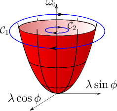
Figure 1: Critical surface of the Dicke model (for the case of a time-independent angle $\phi$) and circular paths chosen in the study of the time-dependent Dicke model.

The focus of our investigation is on a rotationally driven version of the Dicke model Plastina2006 . The unitary transformation

$${\hat{\mathrm{R}}}_{z}(t)=\exp\left[-i\phi(t){\hat{\mathrm{J}}}_{z}\right]$$ (8)

generates a rotation of the spin ${\hat{\mathrm{\bf J}}}$ (of length $j=N/2$) around the $z$ axis with a time-dependent angle $\phi(t)$. Applying this transformation to the Dicke Hamiltonian (1) we get

$${\hat{\mathrm{H}}}_{\mathrm{RD}}(t)={\hat{\mathrm{R}}}_{z}^{\dagger}(t){\hat{\mathrm{H}}}_{\mathrm{D}}{\hat{\mathrm{R}}}_{z}(t)$$

$$=\omega_{0}{\hat{\mathrm{J}}}_{z}+\omega{\hat{\mathrm{a}}}^{\dagger}{\hat{\mathrm{a}}}+\frac{\lambda}{\mathchoice{{\hbox{$\displaystyle\sqrt{2j\,}$}\lower 0.4pt\hbox{\vrule height=6.59525pt,depth=-5.27623pt}}}{{\hbox{$\textstyle\sqrt{2j\,}$}\lower 0.4pt\hbox{\vrule height=6.59525pt,depth=-5.27623pt}}}{{\hbox{$\scriptstyle\sqrt{2j\,}$}\lower 0.4pt\hbox{\vrule height=4.61667pt,depth=-3.69336pt}}}{{\hbox{$\scriptscriptstyle\sqrt{2j\,}$}\lower 0.4pt\hbox{\vrule height=3.29762pt,depth=-2.63812pt}}}}\left({\hat{\mathrm{a}}}^{\dagger}+{\hat{\mathrm{a}}}\right)\left(e^{i\phi(t)}{\hat{\mathrm{J}}}_{+}+e^{-i\phi(t)}{\hat{\mathrm{J}}}_{-}\right).$$ (9)

We choose a linear time dependence

$$\phi(t)=\delta_{\phi}\,t,$$ (10)

so that the two-dimensional vector $(\lambda\cos\phi,\lambda\sin\phi)$ describes a circular motion with constant velocity $\delta_{\phi}$. This is illustrated in Fig. 1, where two distinct paths are shown. The path ${\cal C}_{2}$ lies inside the critical surface, defined by the equation $\omega_{0}=4\lambda^{2}/\omega$, and thus probes the normal phase, while the path ${\cal C}_{1}$ lies outside and probes the superradiant phase, where intriguing dynamical effects appear.

In the following the analysis will be developed for general values of the parameters, but concrete calculations will be carried out at resonance, and we will choose $\omega=\omega_{0}=1$. In this case there remain two relevant parameters, the coupling strength $\lambda$ and the driving velocity $\delta_{\phi}$.

III.2 Dynamics

The rotationally driven Dicke Hamiltonian ${\hat{\mathrm{H}}}_{\mathrm{RD}}(t)$ is obtained by applying a unitary transformation, therefore its eigenvalues are the same as those of the original Hamiltonian ${\hat{\mathrm{H}}}_{\mathrm{D}}$. Nevertheless, the evolution, governed by the time-dependent Schrödinger equation, $i\partial_{t}|{\psi_{\mbox{\scriptsize RD}}(t)}\rangle={\hat{\mathrm{H}}}_{\mathrm{RD}}(t)|{\psi_{\mbox{\scriptsize RD}}(t)}\rangle$ ($\hbar=1$), will lead to novel results, thanks to the combined effects of geometric and dynamic phases. Our approach is to start with a specific initial state at $t=0$ and to let the system evolve according to the Schrödinger equation up to a time $t>0$, where some quantities are measured. A particularly important quantity is the mean photon number

$$n_{\mbox{\scriptsize ph}}(t)=\frac{1}{j}\,\langle{\psi_{\mbox{\scriptsize RD}}(t)}|{\hat{\mathrm{a}}}^{\dagger}{\hat{\mathrm{a}}}|{\psi_{\mbox{\scriptsize RD}}(t)}\rangle,$$ (11)

which in the case of the time-independent Dicke Hamiltonian can be taken as order parameter. Alternatively one may also consider the atomic inversion

$$n_{\mbox{\scriptsize at}}(t)=1+\frac{1}{j}\,\langle{\psi_{\mbox{\scriptsize RD}}(t)}|{\hat{\mathrm{J}}}_{z}|{\psi_{\mbox{\scriptsize RD}}(t)}\rangle.$$ (12)

The sum of these two quantities is just the average number of excitations

$$n_{\mbox{\scriptsize ex}}(t)=\frac{1}{j}\,\langle{\psi_{\mbox{\scriptsize RD}}(t)}|{\hat{\mathrm{N}}}_{\mbox{\scriptsize ex}}|{\psi_{\mbox{\scriptsize RD}}(t)}\rangle.$$ (13)

The analysis is greatly facilitated by a transformation to a co-rotated state,

$$|\psi_{\mbox{\scriptsize ROT}}(t)\rangle={\hat{\mathrm{R}}}_{z}(t)|\psi_{\mbox{\scriptsize RD}}(t)\rangle,$$ (14)

which evolves according to the Schrödinger equation

$$i\partial_{t}|{\psi_{\mbox{\scriptsize ROT}}(t)}\rangle=({\hat{\mathrm{H}}}_{\mathrm{D}}+\delta_{\phi}{\hat{\mathrm{J}}}_{z})|{\psi_{\mbox{\scriptsize ROT}}(t)}\rangle\,.$$ (15)

The operator

$${\hat{\mathrm{H}}}_{\mbox{\scriptsize ROT}}={\hat{\mathrm{H}}}_{\mbox{\scriptsize D}}+\delta_{\phi}\,{\hat{\mathrm{J}}}_{z}$$ (16)

is time-independent and has the form of the Dicke Hamiltonian, with $\omega_{0}$ replaced by the renormalized level splitting

$$\Omega=\omega_{0}+\delta_{\phi}.$$ (17)

Therefore its ground state exhibits a quantum phase transition at $\lambda_{c}=\frac{1}{2}\mathchoice{{\hbox{$\displaystyle\sqrt{\Omega\omega\,}$}\lower 0.4pt\hbox{\vrule height=6.83331pt,depth=-5.46667pt}}}{{\hbox{$\textstyle\sqrt{\Omega\omega\,}$}\lower 0.4pt\hbox{\vrule height=6.83331pt,depth=-5.46667pt}}}{{\hbox{$\scriptstyle\sqrt{\Omega\omega\,}$}\lower 0.4pt\hbox{\vrule height=4.78333pt,depth=-3.82668pt}}}{{\hbox{$\scriptscriptstyle\sqrt{\Omega\omega\,}$}\lower 0.4pt\hbox{\vrule height=3.41666pt,depth=-2.73334pt}}}$ from a normal phase with a vanishing photon density to a superradiant phase with a finite photon density. The critical value $\lambda_{c}$ is expected to play a central role in the time-dependence of physical quantities.

The expectation value of an operator ${\hat{\mathrm{O}}}$ which commutes with ${\hat{\mathrm{J}}}_{z}$ is not affected by the transformation to a co-rotated frame,

$$[{\hat{\mathrm{O}}},{\hat{\mathrm{J}}}_{z}]=0\Rightarrow\,\langle\psi_{\mbox{\scriptsize RD}}(t)|{\hat{\mathrm{O}}}|\psi_{\mbox{\scriptsize RD}}(t)\rangle=\,\langle\psi_{\mbox{\scriptsize ROT}}(t)|{\hat{\mathrm{O}}}|\psi_{\mbox{\scriptsize ROT}}(t)\rangle\,.$$ (18)

This is the case for the quantities mentioned above. If $|\psi_{\mbox{\scriptsize RD}}(0)\rangle$ happens to be an eigenstate of ${\hat{\mathrm{H}}}_{\mbox{\scriptsize ROT}}$, then Eq. (18) implies that $\langle\psi_{\mbox{\scriptsize RD}}(t)|{\hat{\mathrm{O}}}|\psi_{\mbox{\scriptsize RD}}(t)\rangle$ is time-independent. Specifically, if $|\psi_{\mbox{\scriptsize RD}}(0)\rangle$ is the ground state of ${\hat{\mathrm{H}}}_{\mbox{\scriptsize ROT}}$, both the photon density (11) and the fraction of excited atoms (12) will be time-independent and equal to the respective ground state expectation values for ${\hat{\mathrm{H}}}_{\mbox{\scriptsize ROT}}$.

With coherent states, discussed in the next section, expectation values of the operators ${\hat{\mathrm{a}}}$, ${\hat{\mathrm{a}}}^{\dagger}$ and ${\hat{\mathrm{J}}}_{\pm}$ are also relevant. While for the photon creation and annihilation operators the equality (18) holds, this is no longer true in the case of the operators ${\hat{\mathrm{J}}}_{\pm}$, for which we get

$$\langle\psi_{\mbox{\scriptsize RD}}(t)|{\hat{\mathrm{J}}}_{\pm}|\psi_{\mbox{\scriptsize RD}}(t)\rangle=e^{\pm i\phi(t)}\langle\psi_{\mbox{\scriptsize ROT}}(t)|{\hat{\mathrm{J}}}_{\pm}|\psi_{\mbox{\scriptsize ROT}}(t)\rangle\,.$$ (19)

If $|\psi_{\mathrm{RD}}(0)\rangle$ is an eigenstate of ${\hat{\mathrm{H}}}_{\mbox{\scriptsize ROT}}$ the vector $\langle\psi_{\mbox{\scriptsize RD}}(t)|{\hat{\mathrm{\bf J}}}|\psi_{\mbox{\scriptsize RD}}(t)\rangle$ precesses with an angular velocity $\delta_{\phi}$ around the $z$ axis.

III.3 Numerical procedure

We are mostly interested in the thermodynamic limit, $N\rightarrow\infty$, where mean-field theory is expected to produce exact results. In the next Section we will explain in detail how to construct a time-dependent mean-field theory using coherent states. Calculations for a finite number of two-level atoms $N=2j$ (or for a pseudo-spin of finite length $j=N/2$) are nevertheless useful because they allow us both to check the validity of mean-field theory and to study the approach to the thermodynamic limit. In our numerical procedure we truncate the bosonic Hilbert space up to $n_{\mathrm{M}}$ bosons but keep the full $(2j+1)$-dimensional Hilbert space of the spin. We choose $n_{\mathrm{M}}$ always high enough to assure that the error of the numerical data is on the level of the machine precision. In the co-rotating frame the evolution is determined by the time-independent Hamiltonian ${\hat{\mathrm{H}}}_{\mbox{\scriptsize ROT}}$, Eq. (16). To calculate dynamic quantities (18) we use the Chebyshev scheme Tal1984 , where the evolution operator for a small time interval $\Delta t$ is expanded in a Chebyshev series,

$$e^{-i{\hat{\mathrm{H}}}_{\mbox{\scriptsize ROT}}\Delta t}\approx\sum_{k=0}^{M}a_{k}T_{k}({\hat{\mathrm{h}}}),$$ (20)

where $T_{k}({\hat{\mathrm{h}}})$ are the Chebyshev polynomials of order $k$ and ${\hat{\mathrm{h}}}$ is a rescaled Hamiltonian

$${\hat{\mathrm{h}}}=\frac{2{\hat{\mathrm{H}}}_{\mbox{\scriptsize ROT}}-(E_{\mathrm{Max}}+E_{\mathrm{Min}}){\hat{\mathrm{1}}}}{E_{\mathrm{Max}}-E_{\mathrm{Min}}}.$$ (21)

Here $E_{\mathrm{Max}}$ and $E_{\mathrm{Min}}$ are, respectively, the largest and the smallest eigenvalues of ${\hat{\mathrm{H}}}_{\mbox{\scriptsize ROT}}$. The expansion coefficients $a_{k}$ are determined by

$$a_{k}= (-i)^{k}\exp\left(-i\Delta t\frac{1}{2}(E_{\mathrm{Max}}+E_{\mathrm{Min}})\right)(2-\delta_{k,0})$$

$$J_{k}\left(\Delta t\frac{1}{2}(E_{\mathrm{Max}}-E_{\mathrm{Min}})\right),$$ (22)

where $\delta_{k,0}$ is the Kronecker symbol and $J_{k}(x)$ are the Bessel functions of the first kind.

IV Time-dependent mean-field theory

To solve the Schrödinger equation we seek a method which is simple to treat and at the same time becomes exact in the thermodynamic limit. Mean-field theory is believed to reproduce exactly the main features of the equilibrium quantum phase transition of the Dicke model for $j\rightarrow\infty$ castanos , and therefore it should also yield good results for the dynamics in this limit. Mainly two methods have been used for establishing mean-field equations, the coherent-state representation Zhang1990 and the Holstein-Primakoff transformation Emary2003 . These two approaches can be shown to be equivalent in the thermodynamic limit kapor . We adopt the coherent-state representation, using a similar procedure as the one presented in Ref. aguiar .

IV.1 Coherent-state representation

We have seen that for the relevant operators ${\hat{\mathrm{O}}}$ the expectation value $\langle{\psi_{\mbox{\scriptsize RD}}(t)}|{\hat{\mathrm{O}}}|{\psi_{\mbox{\scriptsize RD}}(t)}\rangle$ with an evolution governed by the time-dependent Hamiltonian ${\hat{\mathrm{H}}}_{\mbox{\scriptsize RD}}(t)$ is simply related to $\langle\psi_{\mbox{\scriptsize ROT}}(t)|{\hat{\mathrm{O}}}|\psi_{\mbox{\scriptsize ROT}}(t)\rangle$ with $|\psi_{\mbox{\scriptsize ROT}}(t)\rangle$ evolving according to the time-independent Hamiltonian ${\hat{\mathrm{H}}}_{\mbox{\scriptsize ROT}}$, Eq. (16). For operators commuting with ${\hat{\mathrm{J}}}_{z}$ the two expectation values are the same, while they are transformed to each other by the rotation (19) for the operators ${\hat{\mathrm{J}}}_{\pm}$. In the following we calculate expectation values with respect to co-rotated states and transform the resulting expressions back to the unrotated frame at the end, if necessary. We use the notation

$$\langle{\hat{\mathrm{O}}}\rangle(t):=\langle\psi_{\mbox{\scriptsize ROT}}(t)|{\hat{\mathrm{O}}}|\psi_{\mbox{\scriptsize ROT}}(t)\rangle\,.$$ (23)

The Schrödinger equation (15) leads to

$$\partial_{t}\langle{\hat{\mathrm{O}}}\rangle(t)=i\langle[{\hat{\mathrm{H}}}_{\mbox{\scriptsize ROT}},{\hat{\mathrm{O}}}]\rangle(t)\,.$$ (24)

Specifically we find the equations of motion

$$\partial_{t}\langle{\hat{\mathrm{J}}}_{z}\rangle(t) =\frac{i\lambda}{\mathchoice{{\hbox{$\displaystyle\sqrt{2j\,}$}\lower 0.4pt\hbox{\vrule height=6.59525pt,depth=-5.27623pt}}}{{\hbox{$\textstyle\sqrt{2j\,}$}\lower 0.4pt\hbox{\vrule height=6.59525pt,depth=-5.27623pt}}}{{\hbox{$\scriptstyle\sqrt{2j\,}$}\lower 0.4pt\hbox{\vrule height=4.61667pt,depth=-3.69336pt}}}{{\hbox{$\scriptscriptstyle\sqrt{2j\,}$}\lower 0.4pt\hbox{\vrule height=3.29762pt,depth=-2.63812pt}}}}\langle({\hat{\mathrm{a}}}+{\hat{\mathrm{a}}}^{\dagger})({\hat{\mathrm{J}}}_{-}-{\hat{\mathrm{J}}}_{+})\rangle(t)\,,$$

$$\partial_{t}\langle{\hat{\mathrm{J}}}_{-}\rangle(t) =-i(\omega_{0}+\delta_{\phi})\langle{\hat{\mathrm{J}}}_{-}\rangle(t)+i\mathchoice{{\hbox{$\displaystyle\sqrt{\frac{2}{j}\,}$}\lower 0.4pt\hbox{\vrule height=10.71428pt,depth=-8.57146pt}}}{{\hbox{$\textstyle\sqrt{\frac{2}{j}\,}$}\lower 0.4pt\hbox{\vrule height=7.49998pt,depth=-6.00002pt}}}{{\hbox{$\scriptstyle\sqrt{\frac{2}{j}\,}$}\lower 0.4pt\hbox{\vrule height=5.35713pt,depth=-4.28574pt}}}{{\hbox{$\scriptscriptstyle\sqrt{\frac{2}{j}\,}$}\lower 0.4pt\hbox{\vrule height=5.35713pt,depth=-4.28574pt}}}\lambda\langle({\hat{\mathrm{a}}}+{\hat{\mathrm{a}}}^{\dagger}){\hat{\mathrm{J}}}_{z}\rangle(t)\,,$$

$$\partial_{t}\langle{\hat{\mathrm{a}}}\rangle(t) =-i\omega\langle{\hat{\mathrm{a}}}\rangle(t)-i\frac{\lambda}{\mathchoice{{\hbox{$\displaystyle\sqrt{2j\,}$}\lower 0.4pt\hbox{\vrule height=6.59525pt,depth=-5.27623pt}}}{{\hbox{$\textstyle\sqrt{2j\,}$}\lower 0.4pt\hbox{\vrule height=6.59525pt,depth=-5.27623pt}}}{{\hbox{$\scriptstyle\sqrt{2j\,}$}\lower 0.4pt\hbox{\vrule height=4.61667pt,depth=-3.69336pt}}}{{\hbox{$\scriptscriptstyle\sqrt{2j\,}$}\lower 0.4pt\hbox{\vrule height=3.29762pt,depth=-2.63812pt}}}}\langle({\hat{\mathrm{J}}}_{-}+{\hat{\mathrm{J}}}_{+})\rangle(t)\,.$$ (25)

Those for $\langle{\hat{\mathrm{J}}}_{+}\rangle(t)$ and $\langle{\hat{\mathrm{a}}}^{\dagger}\rangle(t)$ are obtained by complex conjugation.

Our main assumption is now that $|\psi_{\mbox{\scriptsize ROT}}(t)\rangle$ is a coherent state, not only for $t=0$, but also for $t>0$. In the present context this means

$$|\psi_{\mbox{\scriptsize ROT}}(t)\rangle=|\alpha(t)\rangle\otimes|\zeta(t)\rangle=:|\alpha(t),\zeta(t)\rangle$$ (26)

with spin-coherent states

$$|\zeta(t)\rangle=(1+|\zeta(t)|^{2})^{-j}\,e^{\zeta(t){\hat{\mathrm{J}}}_{+}}|j,-j\rangle$$ (27)

and bosonic coherent states

$$|\alpha(t)\rangle=e^{-\frac{1}{2}|\alpha(t)|^{2}}\,e^{\alpha(t)a^{\dagger}}|0\rangle.$$ (28)

The expectation values of the relevant operators with respect to the coherent state (26) are

$$\langle{\hat{\mathrm{J}}}_{+}\rangle(t) =2j\frac{\zeta^{*}(t)}{1+|\zeta(t)|^{2}}=\langle{\hat{\mathrm{J}}}_{-}\rangle^{*}(t)\,,$$

$$\langle{\hat{\mathrm{J}}}_{z}\rangle(t) =-j\,\frac{1-|\zeta(t)|^{2}}{1+|\zeta(t)|^{2}}\,,$$

$$\langle{\hat{\mathrm{a}}}\rangle(t) =\alpha(t)\,,$$

$$\langle{\hat{\mathrm{a}}}^{\dagger}{\hat{\mathrm{a}}}\rangle(t) =|\alpha(t)|^{2}\,.$$ (29)

We note that if $|\psi_{\mbox{\scriptsize ROT}}(t)\rangle$ is a coherent state then this is also true for $|\psi_{\mbox{\scriptsize RD}}(t)\rangle$, which is related to $|\psi_{\mbox{\scriptsize ROT}}(t)\rangle$ by Eq. (14), and vice versa. To see this one verifies that the application of ${\hat{\mathrm{R}}}_{z}^{\dagger}(t)$ on $|\zeta(t)\rangle$ produces a spin-coherent state $|\zeta_{\mbox{\scriptsize RD}}(t)\rangle$ in the original frame with

$$\zeta_{\mbox{\scriptsize RD}}(t)=e^{i\phi(t)}\zeta(t).$$ (30)

IV.2 Classical dynamical system

The equations of motion (25) can now be linked to a classical dynamical system of two coupled oscillators using the parametrization

$$\zeta(t) = \frac{1}{\mathchoice{{\hbox{$\displaystyle\sqrt{4-[Q^{2}(t)+P^{2}(t)]\,}$}\lower 0.4pt\hbox{\vrule height=8.63776pt,depth=-6.91023pt}}}{{\hbox{$\textstyle\sqrt{4-[Q^{2}(t)+P^{2}(t)]\,}$}\lower 0.4pt\hbox{\vrule height=8.63776pt,depth=-6.91023pt}}}{{\hbox{$\scriptstyle\sqrt{4-[Q^{2}(t)+P^{2}(t)]\,}$}\lower 0.4pt\hbox{\vrule height=6.0722pt,depth=-4.85779pt}}}{{\hbox{$\scriptscriptstyle\sqrt{4-[Q^{2}(t)+P^{2}(t)]\,}$}\lower 0.4pt\hbox{\vrule height=4.70554pt,depth=-3.76445pt}}}}\,[Q(t)+iP(t)],$$

$$\alpha(t) = \mathchoice{{\hbox{$\displaystyle\sqrt{\frac{j}{2}\,}$}\lower 0.4pt\hbox{\vrule height=11.7619pt,depth=-9.40956pt}}}{{\hbox{$\textstyle\sqrt{\frac{j}{2}\,}$}\lower 0.4pt\hbox{\vrule height=8.23332pt,depth=-6.58669pt}}}{{\hbox{$\scriptstyle\sqrt{\frac{j}{2}\,}$}\lower 0.4pt\hbox{\vrule height=5.88094pt,depth=-4.70477pt}}}{{\hbox{$\scriptscriptstyle\sqrt{\frac{j}{2}\,}$}\lower 0.4pt\hbox{\vrule height=5.88094pt,depth=-4.70477pt}}}\,[q(t)+ip(t)].$$ (31)

Inserting these relations into Eqs. (25) and isolating real and imaginary parts we find equations of motion

$$\dot{Q} =\Omega P-\lambda q\frac{QP}{\mathchoice{{\hbox{$\displaystyle\sqrt{4-(Q^{2}+P^{2})\,}$}\lower 0.4pt\hbox{\vrule height=8.63776pt,depth=-6.91023pt}}}{{\hbox{$\textstyle\sqrt{4-(Q^{2}+P^{2})\,}$}\lower 0.4pt\hbox{\vrule height=8.63776pt,depth=-6.91023pt}}}{{\hbox{$\scriptstyle\sqrt{4-(Q^{2}+P^{2})\,}$}\lower 0.4pt\hbox{\vrule height=6.0722pt,depth=-4.85779pt}}}{{\hbox{$\scriptscriptstyle\sqrt{4-(Q^{2}+P^{2})\,}$}\lower 0.4pt\hbox{\vrule height=4.70554pt,depth=-3.76445pt}}}}\,,$$ (32)

$$\dot{P} =-\Omega Q+\lambda q\frac{2Q^{2}+P^{2}-4}{\mathchoice{{\hbox{$\displaystyle\sqrt{4-(Q^{2}+P^{2})\,}$}\lower 0.4pt\hbox{\vrule height=8.63776pt,depth=-6.91023pt}}}{{\hbox{$\textstyle\sqrt{4-(Q^{2}+P^{2})\,}$}\lower 0.4pt\hbox{\vrule height=8.63776pt,depth=-6.91023pt}}}{{\hbox{$\scriptstyle\sqrt{4-(Q^{2}+P^{2})\,}$}\lower 0.4pt\hbox{\vrule height=6.0722pt,depth=-4.85779pt}}}{{\hbox{$\scriptscriptstyle\sqrt{4-(Q^{2}+P^{2})\,}$}\lower 0.4pt\hbox{\vrule height=4.70554pt,depth=-3.76445pt}}}}\,,$$

$$\dot{q} =\omega p$$

$$\dot{p} =-\omega q-\lambda Q\mathchoice{{\hbox{$\displaystyle\sqrt{4-(Q^{2}+P^{2})\,}$}\lower 0.4pt\hbox{\vrule height=8.63776pt,depth=-6.91023pt}}}{{\hbox{$\textstyle\sqrt{4-(Q^{2}+P^{2})\,}$}\lower 0.4pt\hbox{\vrule height=8.63776pt,depth=-6.91023pt}}}{{\hbox{$\scriptstyle\sqrt{4-(Q^{2}+P^{2})\,}$}\lower 0.4pt\hbox{\vrule height=6.0722pt,depth=-4.85779pt}}}{{\hbox{$\scriptscriptstyle\sqrt{4-(Q^{2}+P^{2})\,}$}\lower 0.4pt\hbox{\vrule height=4.70554pt,depth=-3.76445pt}}}\,,$$

where $\Omega$ is the renormalized level splitting (17). With the same parametrization the expectation value of ${\hat{\mathrm{H}}}_{\mbox{\scriptsize ROT}}$ yields a classical Hamiltonian $H_{\mbox{\scriptsize cl}}:=\Omega+\frac{1}{j}\langle\alpha(t),\zeta(t)|{\hat{\mathrm{H}}}_{\mbox{\scriptsize ROT}}|\alpha(t),\zeta(t)\rangle$, explicitly

$$H_{\mbox{\scriptsize cl}}=\frac{\Omega}{2}(Q^{2}+P^{2})+\frac{\omega}{2}(q^{2}+p^{2})+\lambda Qq\mathchoice{{\hbox{$\displaystyle\sqrt{4-(Q^{2}+P^{2})\,}$}\lower 0.4pt\hbox{\vrule height=8.63776pt,depth=-6.91023pt}}}{{\hbox{$\textstyle\sqrt{4-(Q^{2}+P^{2})\,}$}\lower 0.4pt\hbox{\vrule height=8.63776pt,depth=-6.91023pt}}}{{\hbox{$\scriptstyle\sqrt{4-(Q^{2}+P^{2})\,}$}\lower 0.4pt\hbox{\vrule height=6.0722pt,depth=-4.85779pt}}}{{\hbox{$\scriptscriptstyle\sqrt{4-(Q^{2}+P^{2})\,}$}\lower 0.4pt\hbox{\vrule height=4.70554pt,depth=-3.76445pt}}}.$$ (33)

Similarly, using Eq. (29) we find for the mean photon number (11)

$$n_{\mbox{\scriptsize ph}}=\frac{1}{j}|\alpha|^{2}=\frac{1}{2}(q^{2}+p^{2})\,,$$ (34)

while the atomic inversion (12) is found to be

$$n_{\mbox{\scriptsize at}}=\frac{2|\zeta|^{2}}{1+|\zeta|^{2}}=\frac{1}{2}(Q^{2}+P^{2})\,.$$ (35)

One readily verifies that Eqs. (32) are the canonical equations for the Hamiltonian (33) and therefore $Q,P,q,p$ are the canonical coordinates of a dynamical system of two degrees of freedom. Once the equations (32) have been solved it is easy to find the corresponding coordinates in the original system using Eq. (30). The photonic variables $q,p$ remain the same, while the atomic variables $Q,P$ become

$$Q_{\mbox{\scriptsize RD}}(t) = Q(t)\cos\phi(t)-P(t)\sin\phi(t)\,,$$

$$P_{\mbox{\scriptsize RD}}(t) = Q(t)\sin\phi(t)+P(t)\cos\phi(t)$$ (36)

in the unrotated frame.

We have verified that the same classical Hamiltonian emerges either when applying the Holstein-Primakoff transformation from spins to bosons or when using the saddle-point approximation of the coherent-state path integral Zhang1990 .

IV.3 Stationary states and linear modes

We show now that the stationary solutions of the classical equations of motion reproduce the phases characterizing the ground state of ${\hat{\mathrm{H}}}_{\mbox{\scriptsize ROT}}$ in the limit $j\rightarrow\infty$. The arguments are similar to those used in Ref. Emary2003 for the time-independent Dicke Hamiltonian. Inserting $\dot{Q}=\dot{P}=\dot{q}=\dot{p}=0$ into Eqs. (32) we find a first obvious solution $Q_{0}=P_{0}=q_{0}=p_{0}=0$ for $\lambda<\lambda_{c}=\frac{1}{2}\mathchoice{{\hbox{$\displaystyle\sqrt{\omega\Omega\,}$}\lower 0.4pt\hbox{\vrule height=6.83331pt,depth=-5.46667pt}}}{{\hbox{$\textstyle\sqrt{\omega\Omega\,}$}\lower 0.4pt\hbox{\vrule height=6.83331pt,depth=-5.46667pt}}}{{\hbox{$\scriptstyle\sqrt{\omega\Omega\,}$}\lower 0.4pt\hbox{\vrule height=4.78333pt,depth=-3.82668pt}}}{{\hbox{$\scriptscriptstyle\sqrt{\omega\Omega\,}$}\lower 0.4pt\hbox{\vrule height=3.41666pt,depth=-2.73334pt}}}$. It describes the normal phase with vanishing photon density. The linearized equations of motion around this point are

$$\dot{Q} =\Omega P\,,$$ (37)

$$\dot{P} =-\Omega Q-2\lambda q\,,$$

$$\dot{q} =\omega p\,,$$

$$\dot{p} =-\omega q-2\lambda Q\,,$$

and the eigenmode frequencies are given by

$$\varepsilon_{\pm}^{2}=\frac{1}{2}\left\{\Omega^{2}+\omega^{2}\pm\mathchoice{{\hbox{$\displaystyle\sqrt{(\Omega^{2}-\omega^{2})^{2}+16\lambda^{2}\Omega\omega\,}$}\lower 0.4pt\hbox{\vrule height=9.30444pt,depth=-7.44359pt}}}{{\hbox{$\textstyle\sqrt{(\Omega^{2}-\omega^{2})^{2}+16\lambda^{2}\Omega\omega\,}$}\lower 0.4pt\hbox{\vrule height=9.30444pt,depth=-7.44359pt}}}{{\hbox{$\scriptstyle\sqrt{(\Omega^{2}-\omega^{2})^{2}+16\lambda^{2}\Omega\omega\,}$}\lower 0.4pt\hbox{\vrule height=6.53888pt,depth=-5.23112pt}}}{{\hbox{$\scriptscriptstyle\sqrt{(\Omega^{2}-\omega^{2})^{2}+16\lambda^{2}\Omega\omega\,}$}\lower 0.4pt\hbox{\vrule height=5.03888pt,depth=-4.03113pt}}}\right\}\,.$$ (38)

$\varepsilon_{-}$ tends to zero for $\lambda\rightarrow\lambda_{c}$ and thus represents the soft mode of the transition.

Two stationary solutions are found for $\lambda>\lambda_{c}$, namely

$$Q_{0} = \pm\mathchoice{{\hbox{$\displaystyle\sqrt{2\,}$}\lower 0.4pt\hbox{\vrule height=6.44444pt,depth=-5.15558pt}}}{{\hbox{$\textstyle\sqrt{2\,}$}\lower 0.4pt\hbox{\vrule height=6.44444pt,depth=-5.15558pt}}}{{\hbox{$\scriptstyle\sqrt{2\,}$}\lower 0.4pt\hbox{\vrule height=4.51111pt,depth=-3.6089pt}}}{{\hbox{$\scriptscriptstyle\sqrt{2\,}$}\lower 0.4pt\hbox{\vrule height=3.22221pt,depth=-2.57779pt}}}\left(1-\frac{{\lambda_{c}}^{2}}{\lambda^{2}}\right)^{\frac{1}{2}}\,,$$

$$q_{0} = \mp\frac{2\lambda}{\omega}\left(1-\frac{{\lambda_{c}}^{4}}{\lambda^{4}}\right)^{\frac{1}{2}}\,,$$

$$P_{0} = p_{0}\,=\,0\,.$$ (39)

They describe the superradiant phase with densities

$$n_{\mbox{\scriptsize ph}} = \frac{1}{j}|\alpha|^{2}=\frac{2\lambda^{2}}{\omega^{2}}\left(1-\frac{{\lambda_{c}}^{4}}{\lambda^{4}}\right)\,,$$

$$n_{\mbox{\scriptsize at}} = \frac{2|\zeta|^{2}}{1+|\zeta|^{2}}=1-\frac{{\lambda_{c}}^{2}}{\lambda^{2}}\,.$$ (40)

We consider small deviations $X=Q-Q_{0}$, $x=q-q_{0}$, $P$, $p$ from the stationary solutions (39) of the superradiant phase. To linear order in these coordinates the equations of motion (32) read

$$\dot{X} =\frac{2}{\omega}(\lambda^{2}+{\lambda_{c}}^{2})P\,,$$ (41)

$$\dot{P} =-\frac{\mathchoice{{\hbox{$\displaystyle\sqrt{8\,}$}\lower 0.4pt\hbox{\vrule height=6.44444pt,depth=-5.15558pt}}}{{\hbox{$\textstyle\sqrt{8\,}$}\lower 0.4pt\hbox{\vrule height=6.44444pt,depth=-5.15558pt}}}{{\hbox{$\scriptstyle\sqrt{8\,}$}\lower 0.4pt\hbox{\vrule height=4.51111pt,depth=-3.6089pt}}}{{\hbox{$\scriptscriptstyle\sqrt{8\,}$}\lower 0.4pt\hbox{\vrule height=3.22221pt,depth=-2.57779pt}}}{\lambda_{c}}^{2}}{\mathchoice{{\hbox{$\displaystyle\sqrt{\lambda^{2}+{\lambda_{c}}^{2}\,}$}\lower 0.4pt\hbox{\vrule height=8.74889pt,depth=-6.99915pt}}}{{\hbox{$\textstyle\sqrt{\lambda^{2}+{\lambda_{c}}^{2}\,}$}\lower 0.4pt\hbox{\vrule height=8.74889pt,depth=-6.99915pt}}}{{\hbox{$\scriptstyle\sqrt{\lambda^{2}+{\lambda_{c}}^{2}\,}$}\lower 0.4pt\hbox{\vrule height=6.14998pt,depth=-4.92001pt}}}{{\hbox{$\scriptscriptstyle\sqrt{\lambda^{2}+{\lambda_{c}}^{2}\,}$}\lower 0.4pt\hbox{\vrule height=4.7611pt,depth=-3.8089pt}}}}x-\frac{8\lambda^{4}}{\omega(\lambda^{2}+{\lambda_{c}}^{2})}X\,,$$

$$\dot{x} =\omega p\,,$$

$$\dot{p} =-\omega x-\frac{\mathchoice{{\hbox{$\displaystyle\sqrt{8\,}$}\lower 0.4pt\hbox{\vrule height=6.44444pt,depth=-5.15558pt}}}{{\hbox{$\textstyle\sqrt{8\,}$}\lower 0.4pt\hbox{\vrule height=6.44444pt,depth=-5.15558pt}}}{{\hbox{$\scriptstyle\sqrt{8\,}$}\lower 0.4pt\hbox{\vrule height=4.51111pt,depth=-3.6089pt}}}{{\hbox{$\scriptscriptstyle\sqrt{8\,}$}\lower 0.4pt\hbox{\vrule height=3.22221pt,depth=-2.57779pt}}}{\lambda_{c}}^{2}}{\mathchoice{{\hbox{$\displaystyle\sqrt{\lambda^{2}+{\lambda_{c}}^{2}\,}$}\lower 0.4pt\hbox{\vrule height=8.74889pt,depth=-6.99915pt}}}{{\hbox{$\textstyle\sqrt{\lambda^{2}+{\lambda_{c}}^{2}\,}$}\lower 0.4pt\hbox{\vrule height=8.74889pt,depth=-6.99915pt}}}{{\hbox{$\scriptstyle\sqrt{\lambda^{2}+{\lambda_{c}}^{2}\,}$}\lower 0.4pt\hbox{\vrule height=6.14998pt,depth=-4.92001pt}}}{{\hbox{$\scriptscriptstyle\sqrt{\lambda^{2}+{\lambda_{c}}^{2}\,}$}\lower 0.4pt\hbox{\vrule height=4.7611pt,depth=-3.8089pt}}}}X\,.$$

The eigenmode frequencies of this linear system are

$$\varepsilon_{\pm}^{2}=\frac{1}{2}\left\{\omega^{2}+\frac{16\lambda^{4}}{\omega^{2}}\pm\mathchoice{{\hbox{$\displaystyle\sqrt{\left(\omega^{2}-\frac{16\lambda^{4}}{\omega^{2}}\right)^{2}+4(\omega\Omega)^{2}\,}$}\lower 0.4pt\hbox{\vrule height=11.80388pt,depth=-9.44315pt}}}{{\hbox{$\textstyle\sqrt{\left(\omega^{2}-\frac{16\lambda^{4}}{\omega^{2}}\right)^{2}+4(\omega\Omega)^{2}\,}$}\lower 0.4pt\hbox{\vrule height=9.30444pt,depth=-7.44359pt}}}{{\hbox{$\scriptstyle\sqrt{\left(\omega^{2}-\frac{16\lambda^{4}}{\omega^{2}}\right)^{2}+4(\omega\Omega)^{2}\,}$}\lower 0.4pt\hbox{\vrule height=6.53888pt,depth=-5.23112pt}}}{{\hbox{$\scriptscriptstyle\sqrt{\left(\omega^{2}-\frac{16\lambda^{4}}{\omega^{2}}\right)^{2}+4(\omega\Omega)^{2}\,}$}\lower 0.4pt\hbox{\vrule height=6.48192pt,depth=-5.18556pt}}}\right\}\,.$$ (42)

The solution with eigenfrequency $\varepsilon_{-}$ again represents a soft mode, $\varepsilon_{-}\rightarrow 0$ for $\lambda\rightarrow\lambda_{c}$. Eqs. (38), (39) and (42) agree with the corresponding expressions for the undriven Dicke model in Ref. Emary2003 , where the Holstein-Primakoff transformation has been used.

This stability analysis shows that in mean-field approximation the rotation applied to the Dicke Hamiltonian changes the phase diagram. The critical point $\lambda_{c}^{0}=\mathchoice{{\hbox{$\displaystyle\sqrt{\omega\omega_{0}\,}$}\lower 0.4pt\hbox{\vrule height=4.30554pt,depth=-3.44446pt}}}{{\hbox{$\textstyle\sqrt{\omega\omega_{0}\,}$}\lower 0.4pt\hbox{\vrule height=4.30554pt,depth=-3.44446pt}}}{{\hbox{$\scriptstyle\sqrt{\omega\omega_{0}\,}$}\lower 0.4pt\hbox{\vrule height=3.01389pt,depth=-2.41113pt}}}{{\hbox{$\scriptscriptstyle\sqrt{\omega\omega_{0}\,}$}\lower 0.4pt\hbox{\vrule height=2.15277pt,depth=-1.72223pt}}}/2$ is shifted to $\lambda_{c}=\mathchoice{{\hbox{$\displaystyle\sqrt{\omega\Omega\,}$}\lower 0.4pt\hbox{\vrule height=6.83331pt,depth=-5.46667pt}}}{{\hbox{$\textstyle\sqrt{\omega\Omega\,}$}\lower 0.4pt\hbox{\vrule height=6.83331pt,depth=-5.46667pt}}}{{\hbox{$\scriptstyle\sqrt{\omega\Omega\,}$}\lower 0.4pt\hbox{\vrule height=4.78333pt,depth=-3.82668pt}}}{{\hbox{$\scriptscriptstyle\sqrt{\omega\Omega\,}$}\lower 0.4pt\hbox{\vrule height=3.41666pt,depth=-2.73334pt}}}/2$, where $\Omega=\omega_{0}+\delta_{\phi}$. The expressions for the photon density and the atomic inversion remain the same as in the time-independent Dicke model, except that $\lambda_{c}^{0}$ is replaced by $\lambda_{c}$. Also the eigenmode frequencies of the time-dependent Dicke Hamiltonian are simply obtained from those of the time-independent Hamiltonian by replacing $\omega_{0}$ by $\Omega$.

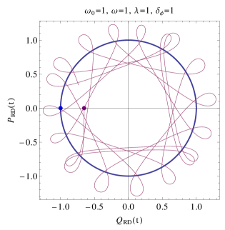
Figure 2: Phase portrait $(Q_{\mbox{\scriptsize{RD}}}(t),P_{\mbox{\scriptsize RD}}(t))$: The blue circle represents the stationary solution in the co-rotating frame, corresponding to the initial condition $Q_{\mbox{\scriptsize{RD}}}(0)=Q_{0},\,P_{\mbox{\scriptsize{RD}}}(0)=0,\,q(0)=q_{0},\,p(0)=0$. The purple trajectory has the initial condition slightly away from the stationary point, i.e., $Q_{\mbox{\scriptsize{RD}}}(0)=Q_{0}+0.347851,\,P_{\mbox{\scriptsize{RD}}}(0)=0,\,q(0)=q_{0},\,p(0)=0$.

The stationary points for the co-rotating frame are readily transformed to the original frame using Eq. (36). The stationary point of the normal phase does not change, but that of the superradiant phase is transformed into uniform circular motion in the $Q_{\mbox{\scriptsize RD}}$-$P_{\mbox{\scriptsize RD}}$ plane with radius $2\mathchoice{{\hbox{$\displaystyle\sqrt{n_{\mbox{\scriptsize at}}\,}$}\lower 0.4pt\hbox{\vrule height=4.30554pt,depth=-3.44446pt}}}{{\hbox{$\textstyle\sqrt{n_{\mbox{\scriptsize at}}\,}$}\lower 0.4pt\hbox{\vrule height=4.30554pt,depth=-3.44446pt}}}{{\hbox{$\scriptstyle\sqrt{n_{\mbox{\scriptsize at}}\,}$}\lower 0.4pt\hbox{\vrule height=3.01389pt,depth=-2.41113pt}}}{{\hbox{$\scriptscriptstyle\sqrt{n_{\mbox{\scriptsize at}}\,}$}\lower 0.4pt\hbox{\vrule height=2.15277pt,depth=-1.72223pt}}}$ and angular velocity $\delta_{\phi}$.

For an initial condition which is close to a stationary point (in the co-rotated frame) the evolution of the system is governed by the linearized equations of motion and will in general be a superposition of harmonic oscillations with frequencies $\varepsilon_{\pm}$. The trajectories form complicated Lissajous patterns, as exemplified in Fig. 2. The purple trajectory (thin line) starting close to the stationary circle (thick line) shows that in addition to the circular motion of angular frequency $\delta_{\phi}$ there is a transverse harmonic oscillation with a frequency $\epsilon_{-}\approx 1-\frac{1}{8\lambda^{4}}=0.875$ (see Appendix A).

V Dynamically generated darkness

We discuss now the evolution after the rotation (8) is switched on suddenly at $t=0$. Thus the system is supposed to be in the ground state $|\psi_{0}\rangle$ of the time-independent Dicke Hamiltonian ${\hat{\mathrm{H}}}_{\mbox{\scriptsize D}}$ for $t<0$ and to evolve according to the time-dependent Dicke Hamiltonian ${\hat{\mathrm{H}}}_{\mbox{\scriptsize RD}}(t)$ for $t>0$. In the rotated frame we have to solve the Schrödinger equation (15) for $|\psi_{\mbox{\scriptsize ROT}}(t)\rangle$ with the initial condition $|\psi_{\mbox{\scriptsize ROT}}(0)\rangle=|\psi_{0}\rangle$. We have used both the numerical technique for the full quantum problem (explained in Section III.3) and the mean-field approximation (described in Section IV) for calculating important quantities such as the photon number and the atomic inversion.

Nothing special will happen for $\lambda<\lambda_{c}^{0}$, where the system starts in the normal phase of ${\hat{\mathrm{H}}}_{\mbox{\scriptsize D}}$ for $t=0$ and proceeds in the normal phase of ${\hat{\mathrm{H}}}_{\mbox{\scriptsize RD}}(t)$ for $t>0$. Therefore we concentrate on couplings $\lambda>\lambda_{c}^{0}$. We use preferentially parameter values $\omega=\omega_{0}=\delta_{\phi}=1$, for which the critical points are $\lambda_{c}^{0}=0.5$ and $\lambda_{c}=1/\mathchoice{{\hbox{$\displaystyle\sqrt{2\,}$}\lower 0.4pt\hbox{\vrule height=6.44444pt,depth=-5.15558pt}}}{{\hbox{$\textstyle\sqrt{2\,}$}\lower 0.4pt\hbox{\vrule height=6.44444pt,depth=-5.15558pt}}}{{\hbox{$\scriptstyle\sqrt{2\,}$}\lower 0.4pt\hbox{\vrule height=4.51111pt,depth=-3.6089pt}}}{{\hbox{$\scriptscriptstyle\sqrt{2\,}$}\lower 0.4pt\hbox{\vrule height=3.22221pt,depth=-2.57779pt}}}\approx 0.707$. For the results presented here we have chosen as initial state the mean-field ground state of ${\hat{\mathrm{H}}}_{\mbox{\scriptsize D}}$, both for the numerical evaluation of the exact quantum dynamics and for the treatment of the classical dynamical system. We have verified that starting with the exact ground state of ${\hat{\mathrm{H}}}_{\mbox{\scriptsize D}}$ (for the numerical procedure) does not modify the main results. The initial values of the classical coordinates $Q(0)$, $q(0)$, $P(0)$ and $p(0)$ are given by Eqs. (39) with $\lambda_{c}$ replaced by $\lambda_{c}^{0}$. In view of Eqs. (31) the corresponding parameters of the initial coherent state are

$$\alpha(0) = \mathchoice{{\hbox{$\displaystyle\sqrt{\frac{j}{2}\,}$}\lower 0.4pt\hbox{\vrule height=11.7619pt,depth=-9.40956pt}}}{{\hbox{$\textstyle\sqrt{\frac{j}{2}\,}$}\lower 0.4pt\hbox{\vrule height=8.23332pt,depth=-6.58669pt}}}{{\hbox{$\scriptstyle\sqrt{\frac{j}{2}\,}$}\lower 0.4pt\hbox{\vrule height=5.88094pt,depth=-4.70477pt}}}{{\hbox{$\scriptscriptstyle\sqrt{\frac{j}{2}\,}$}\lower 0.4pt\hbox{\vrule height=5.88094pt,depth=-4.70477pt}}}q(0)=\mp\frac{\mathchoice{{\hbox{$\displaystyle\sqrt{2j\,}$}\lower 0.4pt\hbox{\vrule height=6.59525pt,depth=-5.27623pt}}}{{\hbox{$\textstyle\sqrt{2j\,}$}\lower 0.4pt\hbox{\vrule height=6.59525pt,depth=-5.27623pt}}}{{\hbox{$\scriptstyle\sqrt{2j\,}$}\lower 0.4pt\hbox{\vrule height=4.61667pt,depth=-3.69336pt}}}{{\hbox{$\scriptscriptstyle\sqrt{2j\,}$}\lower 0.4pt\hbox{\vrule height=3.29762pt,depth=-2.63812pt}}}}{\omega\lambda}\mathchoice{{\hbox{$\displaystyle\sqrt{\lambda^{4}-[\lambda_{c}^{0}]^{4}\,}$}\lower 0.4pt\hbox{\vrule height=9.30444pt,depth=-7.44359pt}}}{{\hbox{$\textstyle\sqrt{\lambda^{4}-[\lambda_{c}^{0}]^{4}\,}$}\lower 0.4pt\hbox{\vrule height=9.30444pt,depth=-7.44359pt}}}{{\hbox{$\scriptstyle\sqrt{\lambda^{4}-[\lambda_{c}^{0}]^{4}\,}$}\lower 0.4pt\hbox{\vrule height=6.53888pt,depth=-5.23112pt}}}{{\hbox{$\scriptscriptstyle\sqrt{\lambda^{4}-[\lambda_{c}^{0}]^{4}\,}$}\lower 0.4pt\hbox{\vrule height=5.03888pt,depth=-4.03113pt}}}\,,$$

$$\zeta(0) = \frac{Q(0)}{\mathchoice{{\hbox{$\displaystyle\sqrt{4-Q^{2}(0)\,}$}\lower 0.4pt\hbox{\vrule height=8.63776pt,depth=-6.91023pt}}}{{\hbox{$\textstyle\sqrt{4-Q^{2}(0)\,}$}\lower 0.4pt\hbox{\vrule height=8.63776pt,depth=-6.91023pt}}}{{\hbox{$\scriptstyle\sqrt{4-Q^{2}(0)\,}$}\lower 0.4pt\hbox{\vrule height=6.0722pt,depth=-4.85779pt}}}{{\hbox{$\scriptscriptstyle\sqrt{4-Q^{2}(0)\,}$}\lower 0.4pt\hbox{\vrule height=4.70554pt,depth=-3.76445pt}}}}=\pm\mathchoice{{\hbox{$\displaystyle\sqrt{\frac{\lambda^{2}-[\lambda_{c}^{0}]^{2}}{\lambda^{2}+[\lambda_{c}^{0}]^{2}}\,}$}\lower 0.4pt\hbox{\vrule height=17.70667pt,depth=-14.16539pt}}}{{\hbox{$\textstyle\sqrt{\frac{\lambda^{2}-[\lambda_{c}^{0}]^{2}}{\lambda^{2}+[\lambda_{c}^{0}]^{2}}\,}$}\lower 0.4pt\hbox{\vrule height=12.43332pt,depth=-9.9467pt}}}{{\hbox{$\scriptstyle\sqrt{\frac{\lambda^{2}-[\lambda_{c}^{0}]^{2}}{\lambda^{2}+[\lambda_{c}^{0}]^{2}}\,}$}\lower 0.4pt\hbox{\vrule height=9.43332pt,depth=-7.54669pt}}}{{\hbox{$\scriptscriptstyle\sqrt{\frac{\lambda^{2}-[\lambda_{c}^{0}]^{2}}{\lambda^{2}+[\lambda_{c}^{0}]^{2}}\,}$}\lower 0.4pt\hbox{\vrule height=9.43332pt,depth=-7.54669pt}}}\,.$$ (43)

Figure 3: Time dependence of the mean photon number at resonance ($\omega=\omega_{0}=1.0$) and for a driving velocity $\delta_{\phi}=1.0$. The red curves (symbols $+$) represent the time evolution of the nonlinear mean-field equations, the green curves (symbols $*$) show the linearized limit of these equations, while the blue curves (symbols $\times$) have been obtained by numerical integration of the Schrödinger equation for a finite system ($j=10$, $n_{\mathrm{M}}=60$). The first two cases (couplings $\lambda=1.3,\,1$) correspond to the superradiant phase of the time-dependent Dicke model, the third ($\lambda=0.6$) to its normal phase. All three couplings exceed the critical value of the time-independent Dicke model ($\lambda_{c}^{0}=0.5$).

Fig. 3 shows results for the mean photon number for three different couplings. Deep in the superradiant phase of ${\hat{\mathrm{H}}}_{\mbox{\scriptsize RD}}$ ($\lambda=1.3$) a simple oscillatory behavior is observed, for both mean-field and full quantum solutions, with $j=10$ in the latter case. This behavior is readily understood in the linearized limit of the mean-field equations, where the coordinates execute harmonic motions, with frequencies $\varepsilon_{\pm}$, as explained in Appendix A. For $\lambda\gg\lambda_{c}$ the main contribution comes from the mode with frequency $\varepsilon_{-}\approx 1-1/{8\lambda^{4}}$, in perfect agreement with Fig. 3. The results for $\lambda=1$ are still reproduced rather well by the linearized dynamics, but not for $\lambda=0.6$, where the anharmonic part of the potential becomes important for the chosen initial conditions. For this coupling the (nonlinear) mean-field behavior agrees only initially with the dynamics obtained from the numerical integration of the Schrödinger equation, but not at later times where the quantum evolution appears to reach a constant value. We attribute this difference to decoherence in the quantum case, for which at longer times than those shown in the figure the initial pattern is restored. Mean-field theory remains by construction a coherent state.

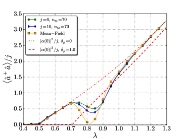
Figure 4: Mean photon number as a function of the coupling strength after a single period of revolution $T_{\phi}$ and for $\omega=\omega_{0}=\delta_{\phi}=1$. Dashed lines represent the ground state values for ${\hat{\mathrm{H}}}_{\mbox{\scriptsize D}}$ and ${\hat{\mathrm{H}}}_{\mbox{\scriptsize ROT}}$, respectively. Full lines have been obtained starting with the ground state of ${\hat{\mathrm{H}}}_{\mbox{\scriptsize D}}$ at $t=0$, but evolving with ${\hat{\mathrm{H}}}_{\mbox{\scriptsize RD}}$ for $0<t<T_{\phi}$, both in mean-field approximation and by numerically solving the Schrödinger equation for finite $j$.

We discuss now the mean photon number $n_{\mbox{\scriptsize ph}}(t)$. If the system evolves according to ${\hat{\mathrm{H}}}_{\mbox{\scriptsize D}}$ and if the initial state $|\psi_{\mathrm{RD}}(0)\rangle$ is the ground state of ${\hat{\mathrm{H}}}_{\mbox{\scriptsize D}}$, then $n_{\mbox{\scriptsize ph}}$ does not depend on time and is just the order parameter of the time-independent Dicke model, except that in the mean-field expression Eq. (40) $\lambda_{c}$ is replaced by $\lambda_{c}^{0}$. An analogous statement holds if the evolution is governed by ${\hat{\mathrm{H}}}_{\mbox{\scriptsize RD}}$ with the ground state of ${\hat{\mathrm{H}}}_{\mbox{\scriptsize ROT}}$ as initial state, then $n_{\mbox{\scriptsize ph}}$ is given by Eq. (40). The two cases are illustrated as dashed lines in Fig. 4. A qualitatively different behavior is found for the scenario discussed above, where the evolution is governed by ${\hat{\mathrm{H}}}_{\mbox{\scriptsize RD}}$, but the initial state is the ground state of ${\hat{\mathrm{H}}}_{\mbox{\scriptsize D}}$. The full lines in Fig. 4 show $n_{\mbox{\scriptsize ph}}$ after a single period of rotation $T_{\phi}:=2\pi/\delta_{\phi}$. For both $\lambda_{c}^{0}<\lambda<\lambda_{c}$ and $\lambda\gg\lambda_{c}$ the mean photon number $n_{\mbox{\scriptsize ph}}(T_{\phi})$ does not differ much from its initial value. For $\lambda$ slightly larger than $\lambda_{c}$ $n_{\mbox{\scriptsize ph}}(T_{\phi})$ is strongly reduced as compared to its value at $t=0$. This remarkable dynamically generated darkness is found both in mean-field approximation and in the quantum evolution for finite $j$.

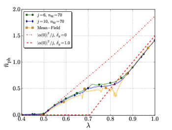
Figure 5: Coupling dependence of the mean photon number averaged over a time $T=150\,T_{\phi}$ for parameter values $\omega=\omega_{0}=\delta_{\phi}=1$. Dashed lines represent the ground state values for ${\hat{\mathrm{H}}}_{\mbox{\scriptsize D}}$ and ${\hat{\mathrm{H}}}_{\mbox{\scriptsize ROT}}$, respectively. The green line (dots) has been obtained by numerically solving the Schrödinger equation for $j=6$ and the blue line (diamonds) for $j=10$ with a cutoff $n_{\mathrm{M}}=70$ in both cases.

The time-averaged mean photon number

$$\bar{n}_{\mbox{\scriptsize ph}}:=\frac{1}{jT}\int_{0}^{T}dt\,\langle\psi(t)|{\hat{\mathrm{a}}}^{\dagger}{\hat{\mathrm{a}}}|\psi(t)\rangle\,$$ (44)

is shown in Fig. 5 for $T\gg T_{\phi}$. In contrast to $n_{\mbox{\scriptsize ph}}(T_{\phi})$, $\bar{n}_{\mbox{\scriptsize ph}}$ approaches the steady state value of ${\hat{\mathrm{H}}}_{\mbox{\scriptsize RD}}$ for $\lambda\gg\lambda_{c}$ (and not that of ${\hat{\mathrm{H}}}_{\mbox{\scriptsize D}}$). This is readily understood in the linearized limit of the classical dynamics, where $q(t)$, $p(t)$ oscillate with a frequency $\varepsilon_{-}\approx\omega$ about the stationary values $q_{0}$, $p_{0}$, as shown in Appendix A. This implies that for $\omega=\delta_{\phi}=1$ the coordinates and thus also $n_{\mbox{\scriptsize ph}}$ recover their original values after a time $T_{\phi}$, in agreement with Fig. 4, but the time-averaged mean photon number $\bar{n}_{\mbox{\scriptsize ph}}$ is close to its stationary value, as in Fig. 5.

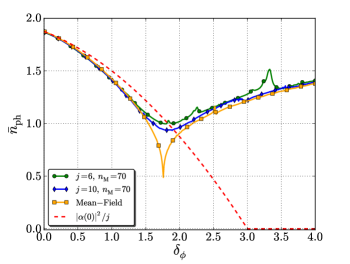
Figure 6: Time-averaged mean photon number (full lines), compared to the initial value (dashed line) as a function of the rotation velocity $\delta_{\phi}$ for $\lambda=\omega=\omega_{0}=1$ and $T=150\,T_{\phi}$. There is a clear minimum, which is very sharp in mean-field approximation (yellow line) and more shallow when calculated numerically for the quantum case with $j=6$ and $j=10$ (green and blue lines, respectively).

Fig. 5 also shows that the reduction of the photon number not only appears at $T_{\phi}$, but is also seen after taking the time average. A clear minimum is found if the time-averaged photon number is plotted as a function of the driving velocity $\delta_{\phi}$ for a fixed coupling strength. This is shown in Fig. 6, where the darkening effect is particularly pronounced in mean-field approximation.

To illustrate the phenomenon of dynamically generated darkness we have studied a simple classical system of a particle moving on a plane in an isotropic potential $V(|{\bf x}|)$ with a maximum $V_{0}$ at the origin and a minimum at $|{\bf x}|=\rho_{0}$ (Mexican hat). Details are described in Appendix B. For a vanishing initial momentum ${\bf p}(0)$ and finite ${\bf x}(0)$ the particle exhibits radial oscillations around $\rho_{0}$ if the energy $E$ is smaller than $V_{0}$, for $E>V_{0}$ it passes over the potential hump at the center and moves back and forth between the turning points $\pm{\bf x}_{\mathrm{max}}$. For $E\approx V_{0}$ the motion is slowed down close to the center, where the particle spends most of the time. The time average of both ${\bf x}^{2}(t)$ and ${\bf p}^{2}(t)$ tends to zero for $E\rightarrow V_{0}$.

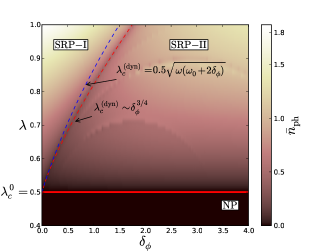
Figure 7: Time-averaged mean photon number as a function of both driving velocity $\delta_{\phi}$ and coupling strength $\lambda$, according to mean-field theory. We have chosen parameter values $\omega=\omega_{0}=1.0$ and averaged over a time $T=150\,T_{\phi}$. The blue dashed line corresponds to the theoretical estimate of Eq. (45), the red dashed line is a fit to the observed minimum.

We use now the result found in the case of the Mexican hat to estimate the critical coupling for maximal slowing down in the case of the time-dependent Dicke model. We expect this to occur if the energy for the given initial conditions is equal to the maximum of the potential at the origin, i.e. $H_{\mbox{\scriptsize cl}}$, given by Eq. (33), vanishes for the coordinates of the stationary state of ${\hat{\mathrm{H}}}_{\mathrm{D}}$. We find the following estimate for this dynamic critical point

$$\lambda_{c}^{\mbox{\scriptsize(dyn)}}\approx\frac{1}{2}\mathchoice{{\hbox{$\displaystyle\sqrt{\omega(\omega_{0}+2\delta_{\phi})\,}$}\lower 0.4pt\hbox{\vrule height=7.5pt,depth=-6.00003pt}}}{{\hbox{$\textstyle\sqrt{\omega(\omega_{0}+2\delta_{\phi})\,}$}\lower 0.4pt\hbox{\vrule height=7.5pt,depth=-6.00003pt}}}{{\hbox{$\scriptstyle\sqrt{\omega(\omega_{0}+2\delta_{\phi})\,}$}\lower 0.4pt\hbox{\vrule height=5.25pt,depth=-4.20003pt}}}{{\hbox{$\scriptscriptstyle\sqrt{\omega(\omega_{0}+2\delta_{\phi})\,}$}\lower 0.4pt\hbox{\vrule height=3.75pt,depth=-3.00002pt}}}\,.$$ (45)

This represents a rough guess because the potential in the case of the Dicke model is both anisotropic and velocity dependent. Therefore it is not surprising that the expression (45) does not reproduce exactly the dynamic critical line found by solving the mean-field equations and shown in Fig. 7. Rather the numerical data are well fitted by a power law, $\lambda_{c}^{\mbox{\scriptsize(dyn)}}=\lambda_{c}^{0}+0.327\,\delta_{\phi}^{3/4}$.

To exemplify the complicated dynamics of the time-dependent Dicke model we present in Fig. 8 a few trajectories, as obtained by solving numerically the equations of motion (32). The stationary states of the time-independent Dicke model have again been chosen as initial conditions. The contour lines in Fig. 8 represent the static limit $V_{\mathrm{cl}}(Q,q,0)$ of the classical potential

$$V_{\mathrm{cl}}(Q,q,P)=\frac{\Omega}{2}Q^{2}+\frac{\omega}{2}q^{2}+\lambda Qq\mathchoice{{\hbox{$\displaystyle\sqrt{4-(Q^{2}+P^{2})\,}$}\lower 0.4pt\hbox{\vrule height=8.63776pt,depth=-6.91023pt}}}{{\hbox{$\textstyle\sqrt{4-(Q^{2}+P^{2})\,}$}\lower 0.4pt\hbox{\vrule height=8.63776pt,depth=-6.91023pt}}}{{\hbox{$\scriptstyle\sqrt{4-(Q^{2}+P^{2})\,}$}\lower 0.4pt\hbox{\vrule height=6.0722pt,depth=-4.85779pt}}}{{\hbox{$\scriptscriptstyle\sqrt{4-(Q^{2}+P^{2})\,}$}\lower 0.4pt\hbox{\vrule height=4.70554pt,depth=-3.76445pt}}}.$$ (46)

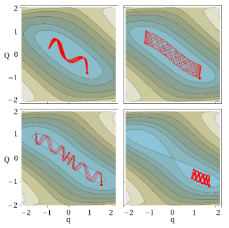
Figure 8: Contours of the potential $V_{\mathrm{cl}}(Q,q,0)$ with the trajectories $(Q,q)$ illustrated by red curves. The red dots mark the initial state given by Eqs. (39) with $\lambda_{c}$ replaced by $\lambda_{c}^{0}$. The four trajectories have been calculated for fixed parameter values $\omega=\omega_{0}=\delta_{\phi}=1$, but different couplings $\lambda=0.6,\,0.72,\,0.823,\,0.9$ (from left to right and top to bottom).

The first trajectory is representative for the range $\lambda_{c}^{0}<\lambda<\lambda_{c}$, where the motion is rather regular, while the fourth trajectory illustrates the strong-coupling region $\lambda\gg\lambda_{c}$, where the motion is limited to the region around one potential minimum. This harmonic motion is correctly reproduced by the linearized limit of the equation of motion. The second trajectory shows the chaotic motion slightly above the critical point ($\lambda=\lambda_{c}$). The third example corresponds to the coupling constant for which $\bar{n}_{\mathrm{ph}}$ has a pronounced minimum according to the mean-field theory ($\lambda=0.823$, see Fig. 5). In this case the trajectory is seen to have inversion symmetry, thus it passes through the origin. However due to the transverse oscillations the motion never stops and therefore the averaged mean photon number is only reduced but does not tend to zero.

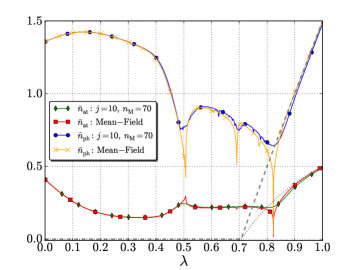
Figure 9: Coupling dependence of the mean photon number and the atomic inversion averaged over a time $T=150T_{\phi}$ for $\omega=\omega_{0}=\delta_{\phi}=1$. Dashed lines represent the ground state values for ${\hat{\mathrm{H}}}_{\mathrm{ROT}}$. The blue line (dots) $\bar{n}_{\mathrm{ph}}$ and green line (diamonds) $\bar{n}_{\mathrm{at}}$ have been calculated by numerically solving the Schrödinger equation for $j=10$ and $n_{\mathrm{M}}=70$. The mean field results, orange line (crosses) for $\bar{n}_{\mathrm{ph}}$ and red line (squares) for $\bar{n}_{\mathrm{at}}$, exhibit sharp features and drop steeply to zero for $\lambda=0.823$. The system is initially in the fine-tuned coherent state with $Q(0)=0.9049$, $P(0)=-1.6382$, $q(0)=-0.0204$, $p(0)=0.171581$.

In the scenario considered above the system is prepared in the ground state of the time-independent Dicke Hamiltonian, then suddenly the rotation is switched on and drives the system out of equilibrium. In that case we have found a reduced photon number but not a complete darkening. We address now the question whether it is possible to fine-tune the initial conditions in such a way that the dynamically generated darkness is complete, i.e. $\bar{n}_{\mathrm{ph}}=0$. To achieve this we simply start at the origin of the coordinate system and also assume that one of the initial momenta vanishes while the other is infinitesimally small. We then follow the evolution for $\lambda=0.823$, the coupling where the previous protocol has provided a minimum in $\bar{n}_{\mathrm{ph}}$. The system remains for a long time close to the initial point in phase space until it moves away and acquires rather large values of both spatial coordinates and momenta. Such a point can then be used as initial condition for other values of $\lambda$. Fig. 9 shows both the mean photon number $\bar{n}_{\mathrm{ph}}$ and the atomic inversion $\bar{n}_{\mathrm{at}}$ as a function of $\lambda$ for the fine-tuned starting point $Q(0)=0.9049$, $P(0)=-1.6382$, $q(0)=-0.0204$, $p(0)=0.171581$. As expected both $\bar{n}_{\mathrm{ph}}$ and $\bar{n}_{\mathrm{at}}$ approach zero for $\lambda=0.823$, or, stated otherwise, there is a complete slowing down at the origin, as in the case of the Mexican hat. Other minima of $\bar{n}_{\mathrm{ph}}$ occur at $\lambda=0.693$ and $\lambda=0.507$, but $\bar{n}_{\mathrm{at}}$ shows the opposite behavior at the latter point, it exhibits a maximum instead of a minimum. For strong couplings both $\bar{n}_{\mathrm{ph}}$ and $\bar{n}_{\mathrm{at}}$ approach the stationary values, as predicted by the solutions of the linearized mean-field equations.

VI Interplay of Geometric and Dynamic Phases

In the previous section we have interpreted the dynamically generated darkness in the framework of time-dependent mean-field theory and attributed the effect to a slowing down of the classical motion. For a system with a small number of two-level atoms mean-field theory is no longer valid and one has to solve the time-dependent Schrödinger equation. We believe that in this case the dynamically generated darkness can be traced back to an interplay between geometric and dynamic phases appearing away from equilibrium TPG . To support this claim we represent the time-dependent Schrödinger equation

$$i\partial_{t}|{\psi_{\mathrm{RD}}(t)}\rangle={\hat{\mathrm{H}}}_{\mathrm{RD}}(t)|{\psi_{\mathrm{RD}}(t)}\rangle$$ (47)

in the instantaneous basis $|{\varphi_{l}(t)}\rangle$ of ${\hat{\mathrm{H}}}_{\mathrm{RD}}(t)$, defined by

$${\hat{\mathrm{H}}}_{\mathrm{RD}}(t)|{\varphi_{l}(t)}\rangle=\epsilon_{l}(t)|{\varphi_{l}(t)}\rangle,$$ (48)

with $l$ enumerating all the eigenstates of ${\hat{\mathrm{H}}}_{\mathrm{RD}}(t)$ at an instant $t$, e.g. $|{\varphi_{1}(t)}\rangle$ is the ground state of ${\hat{\mathrm{H}}}_{\mathrm{RD}}(t)$ at time $t$. The time evolution of the instantaneous eigenstates of ${\hat{\mathrm{H}}}_{\mathrm{RD}}(t)$ is simply given by a rotation of the eigenstates of ${\hat{\mathrm{H}}}_{\mathrm{D}}$, $|{\varphi_{l}(t)}\rangle={\hat{\mathrm{R}}}_{z}^{\dagger}(t)|{\varphi_{l}(0)}\rangle$, with time-independent eigenvalues $\epsilon_{l}(t)=\epsilon_{l}(0)$ (those of ${\hat{\mathrm{H}}}_{\mathrm{D}}$), because the rotationally driven Dicke Hamiltonian ${\hat{\mathrm{H}}}_{\mathrm{RD}}(t)$ is obtained by applying the unitary transformation (8) to the time-independent Dicke Hamiltonian ${\hat{\mathrm{H}}}_{\mathrm{D}}$. Inserting the expansion $|{\psi_{\mathrm{RD}}(t)}\rangle=\sum_{l}c_{l}(t)|{\varphi_{l}(t)}\rangle$ into the Schrödinger equation yields a differential equation for the coefficients $c_{l}(t)$

$$\frac{dc_{l}}{dt}=i\left(-\epsilon_{l}+A_{ll}\right)c_{l}+i\sum_{k,k\neq l}A_{lk}c_{k},$$ (49)

where we introduced the notation $A_{lk}(t):=i\langle{\varphi_{l}(t)}|\frac{d}{dt}|{\varphi_{k}(t)}\rangle$. The integral of the so-called Berry connection $A_{ll}(t)=i\langle{\varphi_{l}(t)}|\frac{d}{dt}|{\varphi_{l}(t)}\rangle$  Xiao2010 is the geometric phase of the $l$-th instantaneous eigenstate, the Berry phase Berry1984

$$\gamma_{l}(t)=\int_{0}^{t}d\tau\,i\,\langle{\varphi_{l}(\tau)}|\frac{d}{d\tau}|{\varphi_{l}(\tau)}\rangle.$$ (50)

Eq. (49) shows that for an adiabatic evolution (where transitions to different levels $k\neq l$ can be neglected) each instantaneous eigenstate $|{\varphi_{l}(t)}\rangle$ acquires not only the well known dynamic phase $\mathcal{E}_{l}(t)=\int_{0}^{t}d\tau\epsilon_{l}$ but also a geometric phase $\gamma_{l}(t)=\int_{0}^{t}d\tau A_{ll}(\tau)$. Applying the gauge transformation

$$c_{l}(t)=\chi_{l}(t)\exp\left(i\int_{0}^{t}d\tau(-\epsilon_{l}+A_{ll}(\tau))\right)$$ (51)

to Eq. (49) we obtain the equation

$$\frac{d\chi_{l}}{dt}=i\sum_{k,k\neq l}A_{lk}(\phi)\exp\left(i\mathcal{E}_{lk}(t)-i\gamma_{lk}(t)\right)\chi_{k}(t),$$ (52)

which emphasizes the interplay between the dynamic phase $\mathcal{E}_{lk}(t)=\mathcal{E}_{l}(t)-\mathcal{E}_{k}(t)$ and the geometric phase $\gamma_{lk}(\phi)=\gamma_{l}(t)-\gamma_{k}(t)$. For our model with a constant rotation speed, $\phi(t)=\delta_{\phi}t$, the characteristic time scale of the drive is $T_{\phi}=2\pi/\delta_{\phi}$. After a single rotation the dynamic phase is given by $\mathcal{E}_{lk}(t)=2\pi(\epsilon_{l}-\epsilon_{k})/\delta_{\phi}$ and is large for $\epsilon_{l}\neq\epsilon_{k}$ if $\delta_{\phi}$ is small. Thus for adiabatic driving ($\delta_{\phi}\to 0$) the level transitions in the dynamics are dictated by the dynamic phase. However, in the case of non-adiabatic driving the geometric phase can affect the transitions and lead to non-trivial phenomena.

As in the previous section we study the evolution after the rotation is switched on suddenly at $t=0$, but now we assume the system to be prepared in the exact ground state of the time-independent Dicke Hamiltonian ${\hat{\mathrm{H}}}_{\mathrm{D}}$. Moreover we now calculate the time evolution of the mean photon number using Eq. (52). The coefficients $\chi_{k}$ are calculated numerically for the initial condition $\chi_{l}(0)=\delta_{l,1}$ and used for evaluating quantities like the photon number

$$n_{\mathrm{ph}}(t)=\frac{1}{j}\sum_{k,l}\chi_{k}^{\ast}(t)\chi_{l}^{\phantom{\ast}}(t)e^{i\mathcal{E}_{kl}(t)-i\gamma_{kl}(t)}\langle{\varphi_{k}(0)}|{\hat{\mathrm{a}}}^{\dagger}{\hat{\mathrm{a}}}|{\varphi_{l}(0)}\rangle.$$ (53)

We also get

$$A_{lk}(\phi)=-\delta_{\phi}\langle{\phi_{l}(0)}|{\hat{\mathrm{J}}}_{z}|{\phi_{k}(0)}\rangle$$ (54)

and therefore a geometric phase

$$\gamma_{l}(t)=\int_{0}^{t}d\tau A_{ll}(\tau)=-\langle{\varphi_{l}(0)}|{\hat{\mathrm{J}}}_{z}|{\varphi_{l}(0)}\rangle\,\phi(t)\,.$$ (55)

We have studied the influence of the geometric phases $\gamma_{l}$ on the dynamics by calculating the mean photon number using Eq. (52) and Eq. (53), once with the values of $\gamma_{l}$ given in Eq. (55), once for $\gamma_{l}=0$ for all levels, $l=1,2,\ldots,(2j+1)(n_{\mathrm{M}}+1)$. The results for $n_{\mathrm{ph}}(T_{\phi})$, shown in Fig. 10, clearly indicate that the minimum of the full solution (green line with dots) disappears if the geometric phases are artificially set to zero (blue line with squares).

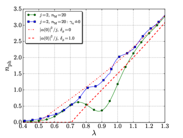
Figure 10: Mean photon number after a single period of revolution $T_{\phi}$ as a function of the coupling and for $\omega=\omega_{0}=\delta_{\phi}=1$. The full lines have been obtained by numerically solving Eq. (52) and using Eq. (53) for $j=2$ with $n_{\mathrm{M}}=20$. The blue line (squares) was calculated by setting all the geometric phases to zero, $\gamma_{l}=0,\,\forall\,l=1,2,\ldots,(2j+1)(n_{\mathrm{M}}+1)$. Dashed lines represent mean-field values for ${\hat{\mathrm{H}}}_{\mathrm{D}}$ and ${\hat{\mathrm{H}}}_{\mathrm{ROT}}$, respectively.

The same effect is seen in the time-averaged photon number, illustrated in Fig. 11, where the darkening is less pronounced. Here we noticed also a difference between the results obtained with and without geometric phases, at small values of $\lambda$. We attribute this disparity to finite size effects, which are expected to be most pronounced for weak coupling. Unfortunately, calculations based on Eq. (52) are hardly practicable for $j>2$. Therefore we were not able to study size dependence using this method.

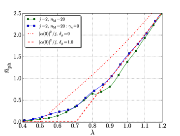
Figure 11: Coupling dependence of the mean photon number averaged over a time $T=10\,T_{\phi}$ and for $\omega=\omega_{0}=\delta_{\phi}=1$. The full lines have been obtained by numerically solving Eq. (52) and time-averaging Eq. (53) for $j=2$ and $n_{\mathrm{M}}=20$. The blue line (squares) was calculated by setting all the geometric phases to zero.

The results of Fig. 10 and 11 show that the geometric phases play an important role in the region slightly above the critical point $\lambda_{c}$. In fact, both for $\lambda_{c}^{0}<\lambda<\lambda_{c}$ and $\lambda\gg\lambda_{c}$ their effect on the photon density seems to be at most marginal. The fact that the minimum disappears if the geometric phases are quenched suggests that these phases are instrumental in the dynamically generated darkness.

VII Conclusion

We have studied the dynamics of a rotationally driven version of the Dicke model, where the collective spin is rotated with a constant velocity about a fixed axis. The main aim was to calculate the effect of the imposed drive on important quantities such as the mean photon number and the atomic inversion. We have used both a numerical technique for the exact quantum dynamics of a finite number of two-level atoms and time-dependent mean-field theory, which is expected to be valid in the thermodynamic limit. The results obtained with these two methods are consistent with each other, although the relatively small size treated numerically does not allow us to draw a definitive conclusion about the limiting behavior of the exact quantum dynamics for arbitrary large system sizes.

Most calculations have been carried out within a co-rotating frame, where the dynamics is governed by a time-independent Dicke model with a renormalized level splitting. In this frame there exists a ground state which undergoes a transition as a function of the coupling strength from a normal phase with vanishing photon number to a superradiant phase with an increasing number of photons (as well as a growing atomic inversion). The critical coupling strength is larger than for the undriven Dicke model and increases with the driving velocity. In the un-rotated frame the expectation value of the collective spin precesses around the static field above the critical point, with the frequency of the drive.

We have studied in great detail the quench dynamics of the driven Dicke model where the system is prepared in the mean-field ground state of the undriven Hamiltonian and then suddenly experiences the rotation. We found a remarkable dynamically generated darkness, a reduction of the photon number due to the rotational driving, both in the numerical calculations for the quantum evolution and in the classical dynamics of the mean-field theory. We have interpreted this phenomenon in two different ways. On the one hand, we have attributed it to a nonlinear slowing down of the classical dynamical system representing time-dependent mean-field theory. On the other hand, for a small number two-level atoms, where the evolution has to be treated quantum mechanically, we identified the geometric phase of the instantaneous eigenstates as the main actor producing the darkening. It would be very interesting to explore possible connections between the two interpretations. Thus one may wonder about the fate of the geometric phase in the mean-field limit. For a very simple quantum-mechanical system the geometric phase has been related to the shift of angle variables in the classical limit Berry1985 , known as Hannay angle Hannay . This angle has been introduced in the context of slowly (adiabatically) cycled integrable systems and therefore cannot be transferred immediately to our model. Future studies may find out whether some classical analogon for the geometric phases of quantum dynamics (Berry phases) are responsible for the dynamically generated darkness reported here.

VIII Acknowledgments

This work was supported by the Swiss National Science Foundation. V.G. is grateful to KITP for hospitality.

Appendix A Solution of the initial value problem for the linearized dynamical system

We consider the classical dynamical system of Section IV.3 and assume the initial deviations from equilibrium - $Q(0)$ and $q(0)$ for the normal phase, $X(0)$ and $x(0)$ for the superradiant phase - to be small, together with $P(0)=p(0)=0$. This allows us to use the linearized equations of motion.

A.1 Normal phase: ${\mathbf{\lambda}<\lambda_{c}}$

For $\lambda<\lambda_{c}$ the linearized equations of motion are given by Eq. (37). In view of the initial conditions $P(0)=p(0)=0$ the general solution is

$$Q(t) = A_{+}\cos(\varepsilon_{+}t)+A_{-}\cos(\varepsilon_{-}t)\,,$$

$$q(t) = a_{+}\cos(\varepsilon_{+}t)+a_{-}\cos(\varepsilon_{-}t)\,,$$ (56)

with eigenmode frequencies $\varepsilon_{\pm}$ given by Eq. (38). Eqs. (37) imply the following relation between coefficients

$$a_{\pm}=f_{\pm}A_{\pm},\quad\mbox{with}\quad f_{\pm}=\frac{\varepsilon_{\pm}^{2}-\Omega^{2}}{2\lambda\Omega}\,.$$ (57)

The initial conditions yield the amplitudes

$$A_{+}=\frac{q(0)-Q(0)f_{-}}{f_{+}-f_{-}}\,,\qquad A_{-}=\frac{Q(0)f_{+}-q(0)}{f_{+}-f_{-}}\,.$$ (58)

A.2 Superradiant phase: ${\mathbf{\lambda}>\lambda_{c}}$

For $\lambda>\lambda_{c}$ the linearized equations of motion (41) describe the deviations $X(t)=Q(t)-Q_{0}$, $x(t)=q(t)-q_{0}$ from the stationary state $Q_{0},\,q_{0}$. The general solution for $P(0)=p(0)=0$ is

$$X(t) = A_{+}\cos(\varepsilon_{+}t)+A_{-}\cos(\varepsilon_{-}t)\,,$$

$$x(t) = a_{+}\cos(\varepsilon_{+}t)+a_{-}\cos(\varepsilon_{-}t)\,$$ (59)

with eigenmode frequencies given by Eq. (42). Using Eqs. (41) we find the following relation between coefficients

$$a_{\pm}=g_{\pm}A_{\pm},\qquad g_{\pm}=\frac{2\mathchoice{{\hbox{$\displaystyle\sqrt{2\,}$}\lower 0.4pt\hbox{\vrule height=6.44444pt,depth=-5.15558pt}}}{{\hbox{$\textstyle\sqrt{2\,}$}\lower 0.4pt\hbox{\vrule height=6.44444pt,depth=-5.15558pt}}}{{\hbox{$\scriptstyle\sqrt{2\,}$}\lower 0.4pt\hbox{\vrule height=4.51111pt,depth=-3.6089pt}}}{{\hbox{$\scriptscriptstyle\sqrt{2\,}$}\lower 0.4pt\hbox{\vrule height=3.22221pt,depth=-2.57779pt}}}\,\omega\lambda_{c}^{2}}{(\varepsilon_{\pm}^{2}-\omega^{2})\mathchoice{{\hbox{$\displaystyle\sqrt{\lambda^{2}+\lambda_{c}^{2}\,}$}\lower 0.4pt\hbox{\vrule height=8.74889pt,depth=-6.99915pt}}}{{\hbox{$\textstyle\sqrt{\lambda^{2}+\lambda_{c}^{2}\,}$}\lower 0.4pt\hbox{\vrule height=8.74889pt,depth=-6.99915pt}}}{{\hbox{$\scriptstyle\sqrt{\lambda^{2}+\lambda_{c}^{2}\,}$}\lower 0.4pt\hbox{\vrule height=6.14998pt,depth=-4.92001pt}}}{{\hbox{$\scriptscriptstyle\sqrt{\lambda^{2}+\lambda_{c}^{2}\,}$}\lower 0.4pt\hbox{\vrule height=4.7611pt,depth=-3.8089pt}}}}\,,$$ (60)

while the initial conditions imply

$$A_{+}=\frac{x(0)-X(0)g_{-}}{g_{+}-g_{-}}\,,\qquad A_{-}=\frac{X(0)g_{+}-x(0)}{g_{+}-g_{-}}\,.$$ (61)

For $\lambda\gg\lambda_{c}$ the coefficient $g_{+}$ is very small and $x(t)\approx a_{-}\cos(\varepsilon_{-}t)$, where $\varepsilon_{-}\approx\omega$.

A.3 Mean photon number

It is now straightforward to calculate some important quantities such as the mean photon number. For simplicity we only consider values averaged over long times and calculate

$$\overline{n}_{\mbox{\scriptsize ph}}=\lim_{T\rightarrow\infty}\frac{1}{2T}\int_{0}^{T}\,dt\,[q^{2}(t)+p^{2}(t)]\,.$$ (62)

We choose the initial conditions of Section V, i.e. $Q(0)$ and $q(0)$ correspond to the stationary state of the time-independent Dicke model. We limit ourselves to the nontrivial case $\lambda>\lambda_{c}^{0}$, where

$$Q(0) = \pm\mathchoice{{\hbox{$\displaystyle\sqrt{2\,}$}\lower 0.4pt\hbox{\vrule height=6.44444pt,depth=-5.15558pt}}}{{\hbox{$\textstyle\sqrt{2\,}$}\lower 0.4pt\hbox{\vrule height=6.44444pt,depth=-5.15558pt}}}{{\hbox{$\scriptstyle\sqrt{2\,}$}\lower 0.4pt\hbox{\vrule height=4.51111pt,depth=-3.6089pt}}}{{\hbox{$\scriptscriptstyle\sqrt{2\,}$}\lower 0.4pt\hbox{\vrule height=3.22221pt,depth=-2.57779pt}}}\left(1-\frac{[\lambda_{c}^{0}]^{2}}{\lambda^{2}}\right)^{\frac{1}{2}}\,,$$

$$q(0) = \mp\frac{2\lambda}{\omega}\left(1-\frac{[\lambda_{c}^{0}]^{4}}{\lambda^{4}}\right)^{\frac{1}{2}}\,.$$ (63)

For $\lambda_{c}^{0}<\lambda<\lambda_{c}$ the system evolves in the normal phase of the time-dependent Dicke model, where the stationary values of the coordinates vanish, $Q_{0}=q_{0}=0$. We obtain

$$\overline{n}_{\mbox{\scriptsize ph}}=\frac{1}{4\omega^{2}}[(\varepsilon_{+}^{2}+\omega^{2})a_{+}^{2}+(\varepsilon_{-}^{2}+\omega^{2})a_{-}^{2}]\,,$$ (64)

where the eigenvalues $\varepsilon_{\pm}$ and coefficients $f_{\pm}$ are given by Eqs. (38) and (58), respectively.

For $\lambda>\lambda_{c}$, i.e. in the superradiant phase of the time-dependent Dicke model, the photon number of the ground state is non-zero and the stationary coordinates $Q_{0},q_{0}$ are given by Eq. (39). The time-dependent coordinates are $q(t)=q_{0}+x(t)$ and $Q(t)=Q_{0}+X(t)$. Therefore the photon number averaged over a long time $T$ is

$$\overline{n}_{\mbox{\scriptsize ph}}=\frac{1}{2}q_{0}^{2}+\frac{1}{4\omega^{2}}[(\varepsilon_{+}^{2}+\omega^{2})a_{+}^{2}+(\varepsilon_{-}^{2}+\omega^{2})a_{-}^{2}]\,,$$ (65)

where $\varepsilon_{\pm}$ and $a_{\pm}$ are defined by Eqs. (42) and (61), respectively, and $x(0)=q(0)-q_{0}$, $X(0)=Q(0)-Q_{0}$.

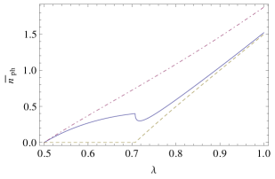
Figure 12: Mean photon number in the linear limit for initial conditions corresponding to the ground state of the time-independent Dicke Hamiltonian and for a subsequent evolution governed by the time-dependent Dicke Hamiltonian with parameters $\omega=\omega_{0}=1,\delta_{\phi}=1$.

The result shown in Fig. 12 is in qualitative agreement with that obtained with the full Hamiltonian (Fig. 5), although the linear approximation cannot be trusted for $\lambda$ of the order of $\lambda_{c}$, where the potential is strongly nonlinear.

Appendix B Slowing down in the Mexican hat

To illustrate the dynamically generated darkness detected for a finite rotation velocity above the critical point of the Dicke model (Section V) we consider a classical system of two degrees of freedom described by the Lagrangian

$$L=\frac{m}{2}(\dot{q}_{1}^{2}+\dot{q}_{2}^{2})+\frac{k}{2}(q_{1}^{2}+q_{2}^{2})-\frac{g}{4}(q_{1}^{2}+q_{2}^{2})^{2}\,,$$ (66)

where $k>0$, $g>0$. In polar coordinates, $q_{1}=\rho\cos\varphi$, $q_{2}=\rho\sin\varphi$, Eq. (66) reads

$$L=\frac{m}{2}(\dot{\rho}^{2}+\rho^{2}\dot{\varphi}^{2})-V(\rho)\,,$$ (67)

where

$$V(\rho)=-\frac{k}{2}\rho^{2}+\frac{g}{4}\rho^{4}$$ (68)

has a minimum $V_{\mbox{\scriptsize min}}=-k^{2}/(4g)$ at $\rho_{0}=\mathchoice{{\hbox{$\displaystyle\sqrt{k/g\,}$}\lower 0.4pt\hbox{\vrule height=7.5pt,depth=-6.00003pt}}}{{\hbox{$\textstyle\sqrt{k/g\,}$}\lower 0.4pt\hbox{\vrule height=7.5pt,depth=-6.00003pt}}}{{\hbox{$\scriptstyle\sqrt{k/g\,}$}\lower 0.4pt\hbox{\vrule height=5.25pt,depth=-4.20003pt}}}{{\hbox{$\scriptscriptstyle\sqrt{k/g\,}$}\lower 0.4pt\hbox{\vrule height=3.75pt,depth=-3.00002pt}}}$. For initial conditions $\dot{q}_{1}(0)=\dot{q}_{2}(0)=0$ a particle moving in this “Mexican hat” executes radial motions, around $\rho_{0}$ if the energy is negative and centered at $\rho=0$ if the energy is positive. In either case the particle spends a lot of time at small values of $\rho$ if the energy is small. To see this quantitatively we consider the special case of a negative energy (for $\dot{\varphi}=0$),

$$\frac{m}{2}\dot{\rho}^{2}-\frac{k}{2}\rho^{2}+\frac{g}{4}\rho^{4}=-\varepsilon$$ (69)

with $\varepsilon>0$, where the particle moves between turning points

$$\rho_{\pm}^{2}=\rho_{0}^{2}\pm\mathchoice{{\hbox{$\displaystyle\sqrt{\rho_{0}^{4}-\frac{4\varepsilon}{g}\,}$}\lower 0.4pt\hbox{\vrule height=9.56943pt,depth=-7.65558pt}}}{{\hbox{$\textstyle\sqrt{\rho_{0}^{4}-\frac{4\varepsilon}{g}\,}$}\lower 0.4pt\hbox{\vrule height=6.6986pt,depth=-5.3589pt}}}{{\hbox{$\scriptstyle\sqrt{\rho_{0}^{4}-\frac{4\varepsilon}{g}\,}$}\lower 0.4pt\hbox{\vrule height=4.7847pt,depth=-3.82777pt}}}{{\hbox{$\scriptscriptstyle\sqrt{\rho_{0}^{4}-\frac{4\varepsilon}{g}\,}$}\lower 0.4pt\hbox{\vrule height=4.7847pt,depth=-3.82777pt}}}\,,$$ (70)

as illustrated in Fig. 13.

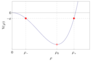
Figure 13: Potential as a function of the radius $\rho$. For a negative energy $-\varepsilon$, the motion is limited by turning points $\rho_{\pm}$ and does not reach the origin.

Eq. (69) then implies

$$dt=\pm\mathchoice{{\hbox{$\displaystyle\sqrt{\frac{2m}{g}\,}$}\lower 0.4pt\hbox{\vrule height=9.56943pt,depth=-7.65558pt}}}{{\hbox{$\textstyle\sqrt{\frac{2m}{g}\,}$}\lower 0.4pt\hbox{\vrule height=6.6986pt,depth=-5.3589pt}}}{{\hbox{$\scriptstyle\sqrt{\frac{2m}{g}\,}$}\lower 0.4pt\hbox{\vrule height=4.7847pt,depth=-3.82777pt}}}{{\hbox{$\scriptscriptstyle\sqrt{\frac{2m}{g}\,}$}\lower 0.4pt\hbox{\vrule height=4.7847pt,depth=-3.82777pt}}}\frac{d\rho}{\mathchoice{{\hbox{$\displaystyle\sqrt{(\rho^{2}-\rho_{-}^{2})(\rho_{+}^{2}-\rho^{2})\,}$}\lower 0.4pt\hbox{\vrule height=7.5pt,depth=-6.00003pt}}}{{\hbox{$\textstyle\sqrt{(\rho^{2}-\rho_{-}^{2})(\rho_{+}^{2}-\rho^{2})\,}$}\lower 0.4pt\hbox{\vrule height=7.5pt,depth=-6.00003pt}}}{{\hbox{$\scriptstyle\sqrt{(\rho^{2}-\rho_{-}^{2})(\rho_{+}^{2}-\rho^{2})\,}$}\lower 0.4pt\hbox{\vrule height=5.25pt,depth=-4.20003pt}}}{{\hbox{$\scriptscriptstyle\sqrt{(\rho^{2}-\rho_{-}^{2})(\rho_{+}^{2}-\rho^{2})\,}$}\lower 0.4pt\hbox{\vrule height=3.75pt,depth=-3.00002pt}}}}\,.$$ (71)

The time $T$ for moving from $\rho_{-}$ to $\rho_{+}$ (or the other way) is

$$T =\mathchoice{{\hbox{$\displaystyle\sqrt{\frac{2m}{g}\,}$}\lower 0.4pt\hbox{\vrule height=9.56943pt,depth=-7.65558pt}}}{{\hbox{$\textstyle\sqrt{\frac{2m}{g}\,}$}\lower 0.4pt\hbox{\vrule height=6.6986pt,depth=-5.3589pt}}}{{\hbox{$\scriptstyle\sqrt{\frac{2m}{g}\,}$}\lower 0.4pt\hbox{\vrule height=4.7847pt,depth=-3.82777pt}}}{{\hbox{$\scriptscriptstyle\sqrt{\frac{2m}{g}\,}$}\lower 0.4pt\hbox{\vrule height=4.7847pt,depth=-3.82777pt}}}\int_{\rho_{-}}^{\rho_{+}}\frac{d\rho}{\mathchoice{{\hbox{$\displaystyle\sqrt{(\rho^{2}-\rho_{-}^{2})(\rho_{+}^{2}-\rho^{2})\,}$}\lower 0.4pt\hbox{\vrule height=7.5pt,depth=-6.00003pt}}}{{\hbox{$\textstyle\sqrt{(\rho^{2}-\rho_{-}^{2})(\rho_{+}^{2}-\rho^{2})\,}$}\lower 0.4pt\hbox{\vrule height=7.5pt,depth=-6.00003pt}}}{{\hbox{$\scriptstyle\sqrt{(\rho^{2}-\rho_{-}^{2})(\rho_{+}^{2}-\rho^{2})\,}$}\lower 0.4pt\hbox{\vrule height=5.25pt,depth=-4.20003pt}}}{{\hbox{$\scriptscriptstyle\sqrt{(\rho^{2}-\rho_{-}^{2})(\rho_{+}^{2}-\rho^{2})\,}$}\lower 0.4pt\hbox{\vrule height=3.75pt,depth=-3.00002pt}}}}$$

$$=\mathchoice{{\hbox{$\displaystyle\sqrt{\frac{2m}{g}\,}$}\lower 0.4pt\hbox{\vrule height=9.56943pt,depth=-7.65558pt}}}{{\hbox{$\textstyle\sqrt{\frac{2m}{g}\,}$}\lower 0.4pt\hbox{\vrule height=6.6986pt,depth=-5.3589pt}}}{{\hbox{$\scriptstyle\sqrt{\frac{2m}{g}\,}$}\lower 0.4pt\hbox{\vrule height=4.7847pt,depth=-3.82777pt}}}{{\hbox{$\scriptscriptstyle\sqrt{\frac{2m}{g}\,}$}\lower 0.4pt\hbox{\vrule height=4.7847pt,depth=-3.82777pt}}}\frac{1}{\rho_{+}}K\left(\frac{\mathchoice{{\hbox{$\displaystyle\sqrt{\rho_{+}^{2}-\rho_{-}^{2}\,}$}\lower 0.4pt\hbox{\vrule height=6.10999pt,depth=-4.88802pt}}}{{\hbox{$\textstyle\sqrt{\rho_{+}^{2}-\rho_{-}^{2}\,}$}\lower 0.4pt\hbox{\vrule height=6.10999pt,depth=-4.88802pt}}}{{\hbox{$\scriptstyle\sqrt{\rho_{+}^{2}-\rho_{-}^{2}\,}$}\lower 0.4pt\hbox{\vrule height=4.30276pt,depth=-3.44223pt}}}{{\hbox{$\scriptscriptstyle\sqrt{\rho_{+}^{2}-\rho_{-}^{2}\,}$}\lower 0.4pt\hbox{\vrule height=3.44165pt,depth=-2.75334pt}}}}{\rho_{+}}\right)\,,$$ (72)

and similarly we obtain

$$\int_{0}^{T}dt\,\rho^{2}(t) =\mathchoice{{\hbox{$\displaystyle\sqrt{\frac{2m}{g}\,}$}\lower 0.4pt\hbox{\vrule height=9.56943pt,depth=-7.65558pt}}}{{\hbox{$\textstyle\sqrt{\frac{2m}{g}\,}$}\lower 0.4pt\hbox{\vrule height=6.6986pt,depth=-5.3589pt}}}{{\hbox{$\scriptstyle\sqrt{\frac{2m}{g}\,}$}\lower 0.4pt\hbox{\vrule height=4.7847pt,depth=-3.82777pt}}}{{\hbox{$\scriptscriptstyle\sqrt{\frac{2m}{g}\,}$}\lower 0.4pt\hbox{\vrule height=4.7847pt,depth=-3.82777pt}}}\int_{\rho_{-}}^{\rho_{+}}\frac{\rho^{2}d\rho}{\mathchoice{{\hbox{$\displaystyle\sqrt{(\rho^{2}-\rho_{-}^{2})(\rho_{+}^{2}-\rho^{2})\,}$}\lower 0.4pt\hbox{\vrule height=7.5pt,depth=-6.00003pt}}}{{\hbox{$\textstyle\sqrt{(\rho^{2}-\rho_{-}^{2})(\rho_{+}^{2}-\rho^{2})\,}$}\lower 0.4pt\hbox{\vrule height=7.5pt,depth=-6.00003pt}}}{{\hbox{$\scriptstyle\sqrt{(\rho^{2}-\rho_{-}^{2})(\rho_{+}^{2}-\rho^{2})\,}$}\lower 0.4pt\hbox{\vrule height=5.25pt,depth=-4.20003pt}}}{{\hbox{$\scriptscriptstyle\sqrt{(\rho^{2}-\rho_{-}^{2})(\rho_{+}^{2}-\rho^{2})\,}$}\lower 0.4pt\hbox{\vrule height=3.75pt,depth=-3.00002pt}}}}$$

$$=\mathchoice{{\hbox{$\displaystyle\sqrt{\frac{2m}{g}\,}$}\lower 0.4pt\hbox{\vrule height=9.56943pt,depth=-7.65558pt}}}{{\hbox{$\textstyle\sqrt{\frac{2m}{g}\,}$}\lower 0.4pt\hbox{\vrule height=6.6986pt,depth=-5.3589pt}}}{{\hbox{$\scriptstyle\sqrt{\frac{2m}{g}\,}$}\lower 0.4pt\hbox{\vrule height=4.7847pt,depth=-3.82777pt}}}{{\hbox{$\scriptscriptstyle\sqrt{\frac{2m}{g}\,}$}\lower 0.4pt\hbox{\vrule height=4.7847pt,depth=-3.82777pt}}}\rho_{+}E\left(\frac{\mathchoice{{\hbox{$\displaystyle\sqrt{\rho_{+}^{2}-\rho_{-}^{2}\,}$}\lower 0.4pt\hbox{\vrule height=6.10999pt,depth=-4.88802pt}}}{{\hbox{$\textstyle\sqrt{\rho_{+}^{2}-\rho_{-}^{2}\,}$}\lower 0.4pt\hbox{\vrule height=6.10999pt,depth=-4.88802pt}}}{{\hbox{$\scriptstyle\sqrt{\rho_{+}^{2}-\rho_{-}^{2}\,}$}\lower 0.4pt\hbox{\vrule height=4.30276pt,depth=-3.44223pt}}}{{\hbox{$\scriptscriptstyle\sqrt{\rho_{+}^{2}-\rho_{-}^{2}\,}$}\lower 0.4pt\hbox{\vrule height=3.44165pt,depth=-2.75334pt}}}}{\rho_{+}}\right)\,,$$ (73)

where $E(k)$ and $K(k)$ are complete elliptic integrals. Therefore the time-average of $\rho^{2}$ is given by

$$\langle\rho^{2}\rangle_{T}:=\frac{1}{T}\int_{0}^{T}dt\,\rho^{2}(t)=\frac{E\left(\frac{\mathchoice{{\hbox{$\displaystyle\sqrt{\rho_{+}^{2}-\rho_{-}^{2}\,}$}\lower 0.4pt\hbox{\vrule height=4.277pt,depth=-3.42162pt}}}{{\hbox{$\textstyle\sqrt{\rho_{+}^{2}-\rho_{-}^{2}\,}$}\lower 0.4pt\hbox{\vrule height=4.277pt,depth=-3.42162pt}}}{{\hbox{$\scriptstyle\sqrt{\rho_{+}^{2}-\rho_{-}^{2}\,}$}\lower 0.4pt\hbox{\vrule height=3.01193pt,depth=-2.40956pt}}}{{\hbox{$\scriptscriptstyle\sqrt{\rho_{+}^{2}-\rho_{-}^{2}\,}$}\lower 0.4pt\hbox{\vrule height=2.40916pt,depth=-1.92735pt}}}}{\rho_{+}}\right)}{K\left(\frac{\mathchoice{{\hbox{$\displaystyle\sqrt{\rho_{+}^{2}-\rho_{-}^{2}\,}$}\lower 0.4pt\hbox{\vrule height=4.277pt,depth=-3.42162pt}}}{{\hbox{$\textstyle\sqrt{\rho_{+}^{2}-\rho_{-}^{2}\,}$}\lower 0.4pt\hbox{\vrule height=4.277pt,depth=-3.42162pt}}}{{\hbox{$\scriptstyle\sqrt{\rho_{+}^{2}-\rho_{-}^{2}\,}$}\lower 0.4pt\hbox{\vrule height=3.01193pt,depth=-2.40956pt}}}{{\hbox{$\scriptscriptstyle\sqrt{\rho_{+}^{2}-\rho_{-}^{2}\,}$}\lower 0.4pt\hbox{\vrule height=2.40916pt,depth=-1.92735pt}}}}{\rho_{+}}\right)}\,\rho_{+}^{2}\,.$$ (74)

For $\varepsilon\rightarrow 0$ the turning point $\rho_{-}$ moves to 0 and the elliptic integrals have the limiting behavior

$$E\left(\frac{\mathchoice{{\hbox{$\displaystyle\sqrt{\rho_{+}^{2}-\rho_{-}^{2}\,}$}\lower 0.4pt\hbox{\vrule height=6.10999pt,depth=-4.88802pt}}}{{\hbox{$\textstyle\sqrt{\rho_{+}^{2}-\rho_{-}^{2}\,}$}\lower 0.4pt\hbox{\vrule height=6.10999pt,depth=-4.88802pt}}}{{\hbox{$\scriptstyle\sqrt{\rho_{+}^{2}-\rho_{-}^{2}\,}$}\lower 0.4pt\hbox{\vrule height=4.30276pt,depth=-3.44223pt}}}{{\hbox{$\scriptscriptstyle\sqrt{\rho_{+}^{2}-\rho_{-}^{2}\,}$}\lower 0.4pt\hbox{\vrule height=3.44165pt,depth=-2.75334pt}}}}{\rho_{+}}\right)\sim 1,\quad K\left(\frac{\mathchoice{{\hbox{$\displaystyle\sqrt{\rho_{+}^{2}-\rho_{-}^{2}\,}$}\lower 0.4pt\hbox{\vrule height=6.10999pt,depth=-4.88802pt}}}{{\hbox{$\textstyle\sqrt{\rho_{+}^{2}-\rho_{-}^{2}\,}$}\lower 0.4pt\hbox{\vrule height=6.10999pt,depth=-4.88802pt}}}{{\hbox{$\scriptstyle\sqrt{\rho_{+}^{2}-\rho_{-}^{2}\,}$}\lower 0.4pt\hbox{\vrule height=4.30276pt,depth=-3.44223pt}}}{{\hbox{$\scriptscriptstyle\sqrt{\rho_{+}^{2}-\rho_{-}^{2}\,}$}\lower 0.4pt\hbox{\vrule height=3.44165pt,depth=-2.75334pt}}}}{\rho_{+}}\right)\sim\log\left(\frac{4\rho_{+}}{\rho_{-}}\right)\,.$$ (75)

It follows that the average value of $\rho^{2}(t)$ tends to zero if $\varepsilon$ tends to zero, i.e. if the initial potential energy coincides with the hump at $\rho=0$. A similar result is obtained for the average $\langle p_{\rho}^{2}\rangle_{T}=m^{2}\langle\dot{\rho}^{2}\rangle_{T}$, which also tends to zero (logarithmically) for $\varepsilon\rightarrow 0$. The origin of this behavior is simply that with decreasing energy the particle slows more and more down by approaching the turning point $\rho_{-}$. At the critical energy (here $\varepsilon=0$), where the motion changes from a simple oscillation about a minimum (for $\varepsilon<0$) to a motion over the potential hump (for $\varepsilon>0$) the time span for a single period diverges and both $\langle\rho^{2}\rangle_{T}$ and $\langle p_{\rho}^{2}\rangle_{T}$ tend to zero. Fig. 14 shows both the analytical expression (74) and numerical results for $\langle\rho^{2}\rangle_{T}$. The agreement is excellent and serves as a test for the algorithm used in the numerical calculations.

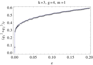
Figure 14: Time average of $q_{1}^{2}(t)+q_{2}^{2}(t)$ at negative energies $-\varepsilon$ for the isotropic “Mexican hat” potential (68) with parameters $m=1$, $k=3$, $g=4$. The full line is the analytical solution, crosses stand for the numerical integration of the equations of motion.

References

- (1) R.H. Dicke, Phys. Rev. 93, 99 (1954).
- (2) M. Tavis and F. W. Cummings, Phys. Rev. 170, 379 (1968); M. Tavis, arXiv:1206.0078.
- (3) K. Hepp and E. H. Lieb, Ann. Phys. 76, 360 (1973).
- (4) Y. K. Wang and F. T. Hioe, Phys. Rev. A 7, 831 (1973).
- (5) H. J. Carmichael, C. W. Gardiner, and D. F. Walls, Phys. Lett. A 46, 47 (1973).
- (6) N. Lambert, C. Emary, and T. Brandes, Phys. Rev. Lett. 92, 073602 (2004); Shi-Biao Zheng, Phys. Rev. A 84, 033817 (2011).
- (7) C. Emary and T. Brandes, Phys. Rev. E 67, 066203 (2003).
- (8) K. Rzazewski, K. Wódkiewicz, and W. Zakowicz, Phys. Rev. Lett. 35, 432 (1975).
- (9) J. Keeling, J. Phys.: Cond. Mat. 19, 295213 (2007).
- (10) A. Vukics and P. Domokos, Phys. Rev. A 86, 053807 (2012).
- (11) F. Dimer, B. Estienne, A. S. Parkins, and H. J. Carmichael, Phys. Rev. A 75, 013804 (2007).
- (12) F. Brennecke, T. Donner, S. Ritter, T. Bourdel, M. Köhl, and T. Esslinger, Nature 450, 268 (2007).
- (13) K. Baumann, C. Guerlin, F. Brennecke, and T. Esslinger, Nature (London) 464, 1301 (2010).
- (14) A. Altland and F. Haake, Phys. Rev. Lett. 108, 073601 (2012).
- (15) A. Altland, V. Gurarie, T. Kriecherbauer, and A. Polkovnikov, Phys. Rev. A 79, 042703 (2009).
- (16) A.P. Itin and P. Törmä, Phys. Rev. A 79, 055602 (2009).
- (17) V. M. Bastidas, C. Emary, B. Regler, and T. Brandes, Phys. Rev. Lett. 108, 043003 (2012).
- (18) E. A. Yuzbashyan, V. B. Kuznetsov, and B. L. Altshuler, Phys. Rev. B 72, 144524 (2005); E. A. Yuzbashyan, O. Tsyplyatyev, and B. L. Altshuler, Phys. Rev. Lett. 96, 097005 (2006).
- (19) O. Tsyplyatyev and D. Loss, Phys. Rev. B 82, 024305 (2010); O. Tsyplyatyev and D. Loss, Phys. Rev. A 80, 023803 (2009).
- (20) Ch. Sträter, O. Tsyplyatyev, and A. Faribault, Phys. Rev. B 86, 195101 (2012).
- (21) F. Plastina, G. Liberti, and A. Carollo, Europhys. Lett., 76, 182 (2006).
- (22) H. Tal-Ezer and R. Kosloff, J. Chem. Phys. 81, 3967 (1984).
- (23) O. Castaños, E. Nahmad-Achar, R. López-Peña, and J. G. Hirsch, Phys. Rev. A 83, 051601 (2011).
- (24) W. Zhang, D.H. Feng, and R. Gilmore, Rev. Mod. Phys. 62, 867 (1990).
- (25) D. V. Kapor, M. J. Škrinjar, and S. D. Stojanović, Phys. Rev. B 44, 2227 (1991).
- (26) M. A. M. de Aguiar, K. Furuya, C. H. Lewenkopf, and M. C. Nemes, Ann. Phys. (New York) 216, 291 (1992).
- (27) M. Tomka, A. Polkovnikov, and V. Gritsev, Phys. Rev. Lett. 108, 080404 (2012).
- (28) D. Xiao, M.-C. Chang, and Q. Niu, Rev. Mod. Phys. 82, 1959 (2010).
- (29) M. V. Berry, Proc. R. Soc. A 392, 45 (1984).
- (30) M. V. Berry, J. Phys. A 18, 15 (1985).
- (31) J. H. Hannay, J. Phys. A 18, 221 (1985).