Online Unsupervised Feature Learning for Visual Tracking

Abstract

Feature encoding with respect to an over-complete dictionary learned by unsupervised methods, followed by spatial pyramid pooling, and linear classification, has exhibited powerful strength in various vision applications. Here we propose to use the feature learning pipeline for visual tracking. Tracking is implemented using tracking-by-detection and the resulted framework is very simple yet effective. First, online dictionary learning is used to build a dictionary, which captures the appearance changes of the tracking target as well as the background changes. Given a test image window, we extract local image patches from it and each local patch is encoded with respect to the dictionary. The encoded features are then pooled over a spatial pyramid to form an aggregated feature vector. Finally, a simple linear classifier is trained on these features.

Our experiments show that the proposed powerful—albeit simple—tracker, outperforms all the state-of-the-art tracking methods that we have tested. Moreover, we evaluate the performance of different dictionary learning and feature encoding methods in the proposed tracking framework, and analyse the impact of each component in the tracking scenario. We also demonstrate the flexibility of feature learning by plugging it into Hare et al.’s tracking method. The outcome is, to our knowledge, the best tracker ever reported, which facilitates the advantages of both feature learning and structured output prediction.

1 Introduction

Robust visual tracking is an important topic in computer vision, with applications to a wide variety of fields, including video surveillance, motion analysis, object recognition, etc. Given the initial state (e.g., bounding box) of a target in a video sequence, a tracking task aims to infer the states of the target in the succeeding frames. Despite significant progress made recently [1, 2, 3, 4, 5, 6, 7, 8], there still exist challenges from various appearance changes of the tracking object to diverse background disturbance. The benchmark work of [9] identifies the influential factors of a test sequence to tracking performance into 11 categories, including illumination variation, occlusion, deformation, motion blur, background clutters, to name a few.

To address the issue of appearance and background variations, many sophisticated appearance models have been proposed, which may roughly be categorized into generative and discriminative based models. Generative models based trackers try to build a robust appearance model of the tracking object and search for the best matched candidate regions. Examples that fall into this category are incremental subspace learning [10], sparse representation based tracking [1, 11, 12, 13, 8], distribution fields representation based tracking [14], etc. In contrast, tracking methods based upon discriminative learning typically model the tracking object as well as the background, followed by a classification decision to distinguish the target from its surroundings. Representatives can be the support vector machines (SVM) [6], boosting ensemble tracking [15], online multiple instance learning [16], bootstrapping binary classifier tracker [17], structured output tracking [2], etc. These methods usually solve the tracking problem as detection (tracking-by-detection). Our proposed tracker applies unsupervised feature learning in an online fashion to model both the tracking target appearance as well as the background, followed by a linear SVM for classification. Hence it belongs to this category.

In recent years, unsupervised feature learning methods have been successfully applied to many vision tasks such as image classification [18, 19, 20], object recognition [21], scene categorization [22]. The classical feature learning pipeline mainly consists of three steps: (a) learning an over-complete dictionary; (b) encoding the features with the learned dictionary; (c) spatially pooling the encoded features over a pyramid of regular spatial grids. The dictionary learning process is typically unsupervised. Methods such as K-means, K-SVD [23], sparse coding, sparse/denoising autoencoder, or even random sampling, can be employed. As for the encoding method, soft threshold, soft assignment, sparse coding, locality-constrained linear coding [24] are commonly applied. It has been shown in [19] that using different dictionary learning methods, even random sampling, has little influence on the classification performance when the dictionary size is sufficiently large, and the pivotal procedure lies in the encoding step. They proved that with a simple soft threshold encoding method, state-of-the-art performance can be achieved in image classification.

The success in those work has inspired us to adapt the image classification pipeline to object tracking. We highlight the main contributions of this work as follows:

• We propose a feature learning based tracker using the online dictionary learning method [25]. The online dictionary learning can adapt to the foreground and background appearance and effectively update the dictionary words. This is important for online problems like tracking. Despite the simplicity of the proposed tracker, it outperforms almost all state-of-the-art trackers in the literature.

• We evaluate the performance of a few widely-used dictionary learning and feature encoding methods in the proposed tracking framework. Due to the nature of tracking problems (such as efficiency requirement and relatively simpler classification compared with generic image classification), some helpful conclusions are made, which deviates from the case of image classification [19].

• To further demonstrate the superior performance of the learned features over traditional hand-crafted features in visual tracking, we incorporate the feature learning part into the Struck tracker [2] and obtain improved tracking accuracy.

2 Related work

As a crucial component of the tracking system, the appearance model has been extensively studied. Besides the traditional hand-crafted features, like texture [15], HOG [26], Haar-like features [16, 17, 2], etc., the sparse representation has been widely used in tracking, which is closely related to our feature learning based tracker proposed here.

In [27, 8], the authors solve the classical sparse coding ($L_{1}$ minimization) problem to sparsely represent the tracking object using a set of target templates and trivial templates. Note that their methods, representations are holistic, and the dictionary is usually constructed using simple methods like sampling or principal component analysis. In contrast, our method is based on local patches. Also no pooling is applied in their methods, which can often significantly improve the accuracy, as shown in our experiments. In their work, the $L_{1}$ minimization problem needs to be solved many times, although [1, 8] applied faster computation to speed up the computation procedure.

Later, the work of [28] contains learning a dictionary on SIFT features extracted from general images (e.g., the VOC2010 and Caltech101 datasets) by solving the sparse coding problem, encoding the feature using the $L_{1}/L_{2}$ sparse coding, then applying max-pooling and training a logistic regression classifier. In addition to the aforementioned issue of extremely expensive computational cost, their method yields a final representation of high dimension (in their case, it is 14336), which can severely hinder its pragmatic value in tracking. The work of [29] proposes to use the histograms of sparse coefficients based on a local sparse dictionary learned from image patches sampled from the first frame of the sequence and then applies mean shift for tracking. Similar work can be found in [11, 12], although the work of [11] adopts a different alignment pooling strategy and in [12], it directly concatenates the learned sparse coefficients instead of pooling. Compared with the methods reviewed above, we show that using online dictionary learning with simple but extremely efficient encoding method, rather than solving the much more expensive $L_{1}$ minimization problem, we can outperform most state-of-the-art trackers.

3 Unsupervised feature learning for tracking

We follow the well-known tracking-by-detection framework [6], which attempts to learn a classifier to discriminate the target object from its background. First, we learn a dictionary ${\bf D}=[{\bf d}_{1},{\bf d}_{2},\ldots,{\bf d}_{n}]\in{\cal R}^{m\times n}$ of size $n$ (each column ${\bf d}_{j}$ denotes a basis vector; if $n>m$, then ${\bf D}$ is over-complete.) based on the image patches extracted from the current frame, and update it online during the tracking when necessary.

Due to its efficiency and being easy-to-implement, the soft threshold (ST) coding strategy is applied here, which writes

$${\bf C}=\max\{0,{\bf D}^{\!\top}{\bf X}-s\}.$$

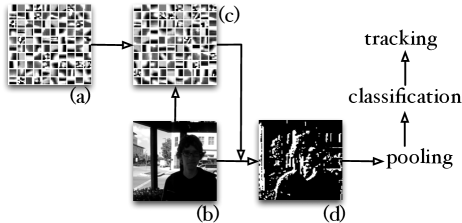
Therefore, ${\bf C}=[{\bf c}_{1},{\bf c}_{2},\ldots,{\bf c}_{n}]^{\!\top}\in{\cal R}^{n\times N}$ are the encoded features, and $s$ is a predefined threshold. We mainly use soft threshold to encode the original features ${\bf X}=[{\bf x}_{1},{\bf x}_{2},\ldots,{\bf x}_{N}]\in{\cal R}^{m\times N}$ (${\bf x}_{i}$ denotes a vector by stacking all pixel values of an image patch). Then we perform the max-pooling operation to produce the final feature vectors, which are used to train a linear SVM for detection. As based on the theoretical and empirical evaluation of [30], max-pooling generally yields more discriminative features for classification, compared to sum or average pooling. The framework of our feature learning based tracking is illustrated in Figure 1 and the algorithm is summarized in Algorithm 1.

Figure 1: An illustration of the pipeline of the proposed feature learning based tracker. Component (a) is the current dictionary before update. Before the tracking starts, (a) is learned from the image patches extracted from the first frame. (c) is the online updated dictionary based on (a) and the local patches from current frame (b). We then encode the local patches in the current frame with respect to the updated dictionary, e.g., using soft threshold encoding. The encoded features (d) are then spatially pooled to form the final features, which are used to train a linear classifier. Tracking is implemented using tracking-by-detection.

3.1 Online dictionary learning

Various dictionary learning techniques exist in the literature, including K-means, K-SVD [23], sparse coding, etc. Recent studies have shown that using relatively simple dictionary learning methods, such as K-means or even random sampling, offers surprisingly promising results in image classification [18, 19]. This is true only when the dictionary size is sufficiently large (typically a few thousand), which leads to high dimensional feature as the dimension of the feature vector is linearly proportional to the dictionary size after the encoding process. For the application of real-time tracking, it requires that the feature dimension cannot be very high for computational efficiency. On the other hand, due to temporal changes in the tracking video, a fixed dictionary is generally not sufficient to cope with the appearance changes of the tracking object as well as the background. We employ online dictionary learning of [25] to build a relatively small-size dictionary by taking both the computational efficiency and online update into consideration.

Given a training set of image patches ${\bf X}$, many classical dictionary learning methods learn an optimized dictionary ${\bf D}$ by (either exactly or approximately) solving the following objective function:

$$\min_{{\bf D},{\boldsymbol{\alpha}}} \sum_{i=1}^{N}{\left[\frac{1}{2}\left\|{\bf x}_{i}-{\bf D}{\boldsymbol{\alpha}}_{i}\right\|_{\mathrm{2}}^{2}+\lambda\left\lVert{\boldsymbol{\alpha}}_{i}\right\rVert_{1}\right]},$$ (1)

$${\rm s.t.} \left\|{\bf d}_{j}\right\|_{\mathrm{2}}^{2}\leq 1,\forall j,$$

where ${\boldsymbol{\alpha}}=[{\boldsymbol{\alpha}}_{1},{\boldsymbol{\alpha}}_{2},\ldots,{\boldsymbol{\alpha}}_{N}]\in{\cal R}^{n\times N}$ are the sparse codes; $\lambda$ is a regularization parameter; $\left\|\cdot\right\|_{\mathrm{2}}$ and $\left\lVert\cdot\right\rVert_{1}$ are the $L_{2}$ and $L_{1}$ norm respectively. The latter enforces sparsity. Problem (1) is not jointly convex with respect to ${\bf D}$ and ${\boldsymbol{\alpha}}$, so it is commonly solved by alternating between the two variables. The online dictionary learning method follows this vein, assuming the training set composed of i.i.d. samples. At each round $t$, the algorithm draws one or more ${\bf x}_{t}$ (${\bf x}_{t,1},\ldots,{\bf x}_{t,\eta}$) and alternates between the classical sparse coding step for computing the sparse code ${\boldsymbol{\alpha}}_{t}$ of ${\bf x}_{t}$ over the dictionary ${\bf D}_{t-1}$, with the dictionary update step for obtaining ${\bf D}_{t}$.

The sparse code ${\boldsymbol{\alpha}}_{t}$ is solved by the LARS-Lasso [31] with ${\bf D}_{t-1}$ fixed:

$${\boldsymbol{\alpha}}_{t}\triangleq\operatornamewithlimits{argmin}_{{\boldsymbol{\alpha}}\in{\cal R}^{n\times\eta}}\frac{1}{\eta}\sum_{j=1}^{\eta}{\left(\frac{1}{2}\left\|{\bf x}_{t,j}-{\bf D}_{t-1}{\boldsymbol{\alpha}}_{j}\right\|_{\mathrm{2}}^{2}+\lambda\left\lVert{\boldsymbol{\alpha}}_{j}\right\rVert_{1}\right)}.$$ (2)

While the dictionary is updated by optimizing:

$${\bf D}_{t} \triangleq\operatornamewithlimits{argmin}_{\left\|{\bf D}\right\|_{\mathrm{2}}^{2}\leq 1}\frac{1}{t\eta}\sum_{i=1}^{t}\sum_{j=1}^{\eta}\left({\frac{1}{2}}\left\|{\bf x}_{i,j}-{\bf D}{\boldsymbol{\alpha}}_{i,j}\right\|_{\mathrm{2}}^{2}+\lambda\left\lVert{\boldsymbol{\alpha}}_{i,j}\right\rVert_{1}\right),$$ (3)

$$=\operatornamewithlimits{argmin}_{\left\|{\bf D}\right\|_{\mathrm{2}}^{2}\leq 1}\frac{1}{t}\left({\frac{1}{2}}\operatornamewithlimits{Tr}({\bf D}^{\!\top}{\bf D}{\bf A}_{t})-\operatornamewithlimits{Tr}({\bf D}^{\!\top}{\bf B}_{t})\right),$$

with

$${\bf A}_{t}= \frac{1}{\eta}\sum_{i=1}^{t}\sum_{j=1}^{\eta}{\boldsymbol{\alpha}}_{i,j}{\boldsymbol{\alpha}}_{i,j}^{\!\top}\triangleq[{\bf a}_{1}^{(t)},\ldots,{\bf a}_{n}^{(t)}],$$ (4)

$${\bf B}_{t}= \frac{1}{\eta}\sum_{i=1}^{t}\sum_{j=1}^{\eta}{\bf x}_{i,j}{\boldsymbol{\alpha}}_{i,j}^{\!\top}\triangleq[{\bf b}_{1}^{(t)},\ldots,{\bf b}_{n}^{(t)}],$$

both of which are also updated online. Here $\operatornamewithlimits{Tr}(\cdot)$ denotes the trace of a matrix, and ${\bf A}_{t}\in{\cal R}^{n\times n}$, ${\bf B}_{t}\in{\cal R}^{m\times n}$. The optimization problem (3) is solved by sequentially updating the $j$-th column of ${\bf D}$ through an orthogonal projection onto the constrained set:

$${\bf d}_{j}^{(t)}\leftarrow\frac{1}{\max(\left\|{\bf u}_{j}\right\|_{\mathrm{2}},1)}{\bf u}_{j},$$ (5)

where ${\bf u}_{j}=\frac{1}{{\bf A}_{t}[j,j]}\left({\bf b}_{j}^{(t)}-{\bf D}_{t-1}{\bf a}_{j}^{(t)}\right)+{\bf d}_{j}^{(t-1)}$, with ${\bf A}_{t}[j,j]$ denotes the $j$-th row and $j$-th column element of ${\bf A}_{t}$, and ${\bf d}_{j}^{(t-1)}$, ${\bf d}_{j}^{(t)}$ is the $j$-th column of ${\bf D}_{t-1}$ and ${\bf D}_{t}$ respectively.

The algorithm is summarized in Algorithm 2. It is worth noting that the method can also be used in an off-line fashion to train on fixed-size data by cycling over a randomly permuted training set to draw ${\bf x}_{t}$. In the tracking task, the dictionary can be off-line learned from natural images or the first frame of the sequence. We provide a comparison of these three cases in the experiment section.

Dictionary update

To avoid the unstable performance caused by too frequent update as well as to ensure efficiency, we apply some heuristic strategies here. To capture the appearance change of the object, we introduce a weighting scheme for each basis in ${\bf D}$, which is defined as the normalized $L_{2}$ norm of the encoded features. Specifically, the $j$-th basis ${\bf d}_{j}$ is weighted as $\frac{\left\|{\bf c}_{j}\right\|_{\mathrm{2}}}{\sum_{j=1}^{n}{\left\|{\bf c}_{j}\right\|_{\mathrm{2}}}}$. It indicates the relative importance of the bases in the encoding process, and essentially the appearance of the region. According to this weighting scheme, we can sort the bases from the most important to the least important. During the tracking, if the overlap between the top half bases of the two detected target regions in consecutive frames below a threshold ($0.9$ in our experiment), then there is possibly appearance change happening, and the dictionary is updated. We give an illustration by visualizing the ordered learned bases (100 in total) with their corresponding encoded responses in figure 2. As can be seen, the ranked bases provide some intuitive insights into the feature learning approach.

Figure 2: The image frame and the learned bases (first row) ordered by the weighting skeme from most important to least important and their corresponding encoded features/responses (second row). The rank is 1st, 20th, 40th, 60th, 80th, 100th from left to right.

Algorithm 1 Online feature learning based tracking.

Input:

Initial dictionary ${\bf D}_{0}$; image patch size $p$; step size $q$; length of sequence $T$.

Initialize: ${\bf A}_{0}\leftarrow 0,{\bf B}_{0}\leftarrow 0$.

for $t=1$ to $T$ do

$\bf\cdot$ Extract image patches ${\bf x}_{t,1},\ldots,{\bf x}_{t,\eta}$ of size $p\times p$ at step size $q$ from frame $t$ and do contrast normalization.

$\bf\cdot$ Update dictionary ${\bf D}_{t}$ by calling Algorithm 2.

$\bf\cdot$ Sample a bunch of boxes around the previous estimation of the tracking target.

$\bf\cdot$ Encode the raw pixel features of the patches extracted within each sampled boxes using ${\bf D}_{t}$ by soft threshold coding.

$\bf\cdot$ Perform max-pooling over a spatial pyramid of multiple layers.

$\bf\cdot$ Train an LS-SVM by solving (7).

$\bf\cdot$ Predict the most confident bounding box of the tracking target.

end for

Algorithm 2 Dictionary update.

Input:

Training samples ${\bf x}_{t,1},\ldots,{\bf x}_{t,\eta}\in{\cal R}^{m}$; regularization parameter $\lambda$; ${\bf A}_{t-1}$; ${\bf B}_{t-1}$; ${\bf D}_{t-1}$.

$\bf\cdot$ Solve Eq. (2) for ${\boldsymbol{\alpha}}$.

$\bf\cdot$ Update ${\bf A}_{t}$: ${\bf A}_{t}\leftarrow{\bf A}_{t-1}+\frac{1}{\eta}\sum_{i=1}^{\eta}{\boldsymbol{\alpha}}_{t,i}{\boldsymbol{\alpha}}_{t,i}^{\!\top}$;

$\bf\cdot$ Update ${\bf B}_{t}$: ${\bf B}_{t}\leftarrow{\bf B}_{t-1}+\frac{1}{\eta}\sum_{i=1}^{\eta}{\bf x}_{t,i}{\boldsymbol{\alpha}}_{t,i}^{\!\top}$;

$\bf\cdot$ for $j=1$ to $n$ do

$\bf\cdot$  Update the $j$-th column of ${\bf D}_{t-1}$ by (5);

$\bf\cdot$ end for ;

Output:

The updated dictionary ${\bf D}_{t}$.

3.2 Re-training of linear classification

To build an appearance discriminative model, we train a linear least-squared SVM (LS-SVM) classifier on the learned features, mainly due to its fast closed-form solution. Of course many other classifiers can be used here.

Given a set of training examples $\{{\bf x}_{i},y_{i}\}_{i=1}^{N}$, where ${\bf x}_{i}\in{\cal R}^{m}$ and $y_{i}\in\{-1,+1\}$, the LS-SVM learns a classifier $f({\bf x})={\bf w}^{\!\top}{\bf x}+b$ by optimizing the following objective function [32]:

$$\min_{{\bf w},b}\sum_{i=1}^{N}\left\|f({\bf x}_{i})-y_{i}\right\|_{\mathrm{2}}^{2}+\gamma\left\|{\bf w}\right\|_{\mathrm{2}}^{2},$$ (6)

where $\left\|\cdot\right\|_{\mathrm{2}}$ is the $L_{2}$ norm and $\gamma$ is the trade-off parameter. To simplify notation, we define ${\bf 1}$ as an vector of all ones, ${\bf X}=[{\bf x}_{1},{\bf x}_{2},\ldots,{\bf x}_{N}]$ to be the data matrix, $N_{+},N_{-}$ be the positive and negative sample number respectively, ${\boldsymbol{\mu}}_{+},{\boldsymbol{\mu}}_{-}$ be the positive and negative sample mean, and ${\boldsymbol{\mu}}$ be the mean of all training samples. Obviously we have $N=N_{+}+N_{-}$ and ${\boldsymbol{\mu}}=\frac{N_{+}}{N}{\boldsymbol{\mu}}_{+}+\frac{N_{-}}{N}{\boldsymbol{\mu}}_{-}$. Then the closed form solution of (6) can be formulated as:

$${\bf w} =\frac{2N_{+}N_{-}}{N^{2}}({\bf S}+\frac{\gamma}{N}{\bf I})^{-1}({\boldsymbol{\mu}}_{+}-{\boldsymbol{\mu}}_{-}),$$ (7)

$$b =\frac{N_{+}N_{-}}{N}-{\boldsymbol{\mu}}^{\!\top}{\bf w},$$

where ${\bf I}$ is an identity matrix and ${\bf S}$ is the covariance matrix formulated as ${\bf S}=\frac{1}{N}({\bf X}-{\boldsymbol{\mu}}{\bf 1}^{\!\top})({\bf X}-{\boldsymbol{\mu}}{\bf 1}^{\!\top})^{\!\top}$. During tracking, we use an online reservoir of boxes from a maximum number of frames (30 in our experiment) for training. Generally, the earliest tracking results are more accurate, while the latest ones capture the recent appearance of the tracking target. Based on these two considerations, we select the boxes from the first 10 together with the most recent 20 frames to maintain the reservoir.

4 Experiments

In this section, we offer a comprehensive evaluation of the proposed tracker on twenty sequences, most of which can be found at the website of the first author of [9]. These sequences contain various challenging situations in object tracking, like illumination variation, occlusion, deformation, background clutters, fast motion etc. For a detailed attribute description, please refer to [9]. Two widely-used evaluation criteria are utilized here, namely, the center location error (CLE) and the PASCAL VOC overlap ratio (VOR), with the latter defined as ${\rm VOR}={{\rm area}(S_{T}\bigcap S_{GT})}/{{\rm area}(S_{T}\bigcup S_{GT})}$, where $S_{T}$ is the tracking result box and $S_{GT}$ the ground truth bounding box.

We use a search radius of 30 for tracking and 60 for training classifier, as did in Struck [2]. The dictionary is initially learned from image patches of the first frame and then online updated. We extract $8\times 8$ patches at a step size 4 for large tracking objects and $6\times 6$ with stride 2 for small targets. The patches are then normalized by subtracting the mean and dividing by the standard deviation for contrast normalization. Note that we do not do the unit length normalization here as it degrades performance. We use a dictionary size of 100 ($n=100$) and soft threshold (ST) coding with three-level max pooling ($1\times 1,2\times 2,3\times 3$), which yields a feature dimension of 1400. As we do not do the unit length normalization, we empirically set the threshold of ST as $s=0.25\cdot\max{({\bf D}^{\!\top}{\bf X})}$ and use it throughout all the sequences. We use the optimization toolbox [25] for online updating the dictionary and solving the sparse coding problem.

During the tracking, we maintain a reservoir of 30 frames (the first 10 and the most recent 20; fixed for all the sequences) for re-training the LS-SVM. The classifier is initially trained with the first two labelled frames and updated every four frames. Our unoptimized Matlab implementation runs around 4 frames per second with no dictionary updating and around 2.5 frames per second with dictionary update, on a standard PC machine using a single core.

4.1 Comparison with state-of-the-art trackers

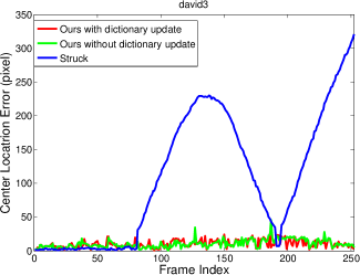
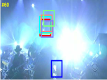
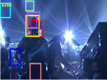
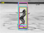
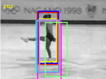
We first compare our tracker with eight state-of-the-art trackers, which are Struck (structured output tracker [2]), SCM (sparsity-based collaborative model [12]), ASLA (adaptive structural local appearance model [11]), L1APG ($L_{1}$ tracker using accelerated proximal gradient approach [1]), DFT (distribution field tracker [14]), MTT (multi-task sparse learning tracker [13]), TLD (bootstrapping binary classifier tracker [17]), IVT (incremental subspace tracker [10]). The publicly available benchmark code of [9] with initial settings are used for evaluating their results. We report the average VORs and CLEs in Table 1 and Table 2 respectively. For our method, due to the randomness introduced by the dictionary learning process, we run 5 times and report the median results. The results of our tracker both with and without dictionary update process are included in the table. From the results, we can see that our tracker with online dictionary update achieves the best overall performance across all the twenty sequences, especially on the david3, box, iceball and bolt, where the other trackers lose the target at different frames. One more notable conclusion is that even without dictionary update, our tracker performs surprisingly well, which may result from the fact that most tracking scenes consist of relatively simple image patterns. We will give more discussions on the dictionary update later.

Sequence	Ours	Ours_U	Struck [2]	SCM [12]	ASLA [11]	L1APG [1]	DFT [14]	MTT [13]	TLD [17]	IVT [10]
david	0.85	0.86	0.79	0.61	0.59	0.40	0.48	0.30	0.59	0.47
girl	0.79	0.81	0.80	0.42	0.63	0.73	0.39	0.62	0.42	0.04
faceocc1	0.80	0.80	0.83	0.92	0.86	0.78	0.51	0.69	0.65	0.78
faceocc2	0.81	0.82	0.74	0.74	0.74	0.75	0.82	0.75	0.48	0.66
david3	0.73	0.73	0.29	0.48	0.49	0.38	0.56	0.10	0.28	0.49
woman	0.71	0.72	0.74	0.32	0.15	0.16	0.76	0.17	0.28	0.14
shaking	0.71	0.71	0.08	0.55	0.64	0.36	0.14	0.55	0.12	0.03
fskater	0.80	0.81	0.81	0.59	0.73	0.67	0.67	0.77	0.51	0.62
bird2	0.78	0.78	0.55	0.75	0.51	0.43	0.74	0.08	0.23	0.48
deer	0.73	0.75	0.74	0.10	0.05	0.60	0.26	0.66	0.25	0.03
dollar	0.82	0.82	0.70	0.85	0.87	0.80	0.86	0.87	0.30	0.87
box	0.81	0.82	0.34	0.17	0.13	0.22	0.34	0.26	0.52	0.55
board	0.81	0.82	0.76	0.36	0.69	0.08	0.34	0.19	0.24	0.15
coke11∗	0.55	0.59	0.55	0.50	0.18	0.10	0.16	0.43	0.41	0.05
tiger1∗	0.74	0.73	0.71	0.12	0.29	0.44	0.36	0.38	0.39	0.09
tiger2∗	0.74	0.73	0.59	0.27	0.13	0.26	0.57	0.30	0.31	0.13
sylvester∗	0.75	0.73	0.69	0.56	0.59	0.41	0.50	0.71	0.66	0.54
trellis∗	0.78	0.77	0.79	0.61	0.75	0.43	0.37	0.44	0.33	0.15
iceball∗	0.70	0.72	0.51	0.48	0.45	0.49	0.08	0.06	0.07	0.06
bolt∗	0.71	0.73	0.01	0.02	0.01	0.01	0.03	0.01	0.16	0.01
average	0.75	0.76	0.60	0.47	0.47	0.43	0.45	0.42	0.36	0.32

Table 1: Compared average VORs on 20 sequences. Ours_U and Ours refer to our tracker with and without dictionary update respectively. The last row are the averaged results on all sequences. The best and second best are shown in red and blue respectively. The sequences marked with star (*) are evaluated by using a patch size of 6 and stride 2 due to small target objects and all the other sequences use a patch size of 8 with stride 4.

Sequence	Ours	Ours_U	Struck [2]	SCM [12]	ASLA [11]	L1APG [1]	DFT [14]	MTT [13]	TLD [17]	IVT [10]
david	5.7	5.2	8.8	5.8	2.9	44.9	55.8	93.8	8.1	3.9
girl	12.1	10.4	10.2	60.5	30.3	13.1	51.2	23.3	31.7	145.5
faceocc1	12.0	11.6	7.5	4.1	7.1	13.0	47.3	20.6	19.0	12.8
faceocc2	9.1	8.7	9.2	8.4	9.3	8.2	8.5	10.1	16.3	7.9
david3	10.3	10.1	106.7	75.6	85.6	90.0	51.0	399.2	135.7	51.6
woman	5.4	5.2	4.1	118.8	157.7	128.7	8.5	138.1	78.9	181.6
shaking	10.6	10.8	123.9	18.1	11.6	84.5	174.8	18.2	65.6	86.7
fskater	10.5	9.2	7.1	26.3	8.1	21.2	22.8	12.3	15.9	19.4
bird2	7.6	7.7	20.7	8.7	22.1	57.6	10.7	145.6	75.1	30.7
deer	8.2	7.9	5.3	108.3	144.2	24.2	98.7	11.9	117.7	179.4
dollar	7.5	6.6	14.7	5.2	4.2	6.9	5.0	5.2	70.0	5.0
box	9.4	8.9	140.0	127.1	165.7	104.1	106.2	100.6	20.7	18.3
board	16.7	15.5	24.0	100.9	34.3	220.0	98.3	142.8	130.8	157.4
coke11∗	8.1	7.4	8.3	10.9	29.5	64.1	30.2	17.9	14.1	44.5
tiger1∗	5.4	5.7	6.0	86.1	32.9	23.2	30.5	26.9	22.4	60.3
tiger2∗	6.4	6.2	9.2	25.9	41.2	35.4	12.5	24.3	17.7	44.7
sylvester∗	6.7	7.1	8.4	19.8	21.0	41.9	36.1	7.1	8.6	36.7
trellis∗	5.2	6.2	5.0	15.0	7.1	41.6	54.6	43.9	41.0	156.7
iceball∗	4.9	4.5	15.6	32.0	18.3	14.4	116.6	137.3	101.5	106.0
bolt∗	6.9	6.6	365.2	374.6	385.3	408.4	367.3	485.6	88.0	379.4
average	8.4	8.1	45.0	61.6	60.9	72.3	69.3	93.2	53.9	86.4

Table 2: Compared average CLEs in pixels on 20 sequences. Ours_U and Ours refer to our tracker with and without dictionary update respectively. The last row are the averaged results on all sequences. The best and second best are shown in red and blue respectively. The sequences marked with star (*) are evaluated by using a patch size of 6 and stride 2 due to small target objects and all the other sequences use a patch size of 8 with stride 4.

4.2 Analysis of feature learning

In this section, we examine several factors that have impact on the performance of the proposed tracker.

Evaluation of different dictionary learning methods

We compare the online dictionary learning algorithm [25] used in this paper with two other typical dictionary learning methods, namely, K-means and K-SVD [23]. We also include results using random sampled (RS) patches as dictionary, and all the methods use the image patches extracted from the first frame. One may suspect using patches obtained from natural images may yield better performance, as they may provide more general patterns. To justify this point, we also run the ODL method by utilizing 100000 image patches randomly selected from a segmentation database and use it through out all the sequences. The dictionary size is fixed at 100 for all the methods. Table 3 shows the average VORs and CLEs on eight sequences. The results indicate that the random sample method performs bad in the case of small dictionary size, and using different dictionary learning methods has little influence in the tracking performance, which is in accordance with the conclusion of [19] in image classification. The reason why we use ODL rather than the other two is that K-SVD is more time consuming and K-means suffers from unstable performance in case of online update. One more conclusion can be made from Table 3 is that using image patches directly from the sequence can better capture the patterns of the tracking object as well as the background, especially when the dictionary size is not large enough.

Sequence	ODL_G		ODL		K-means		K-SVD		RS
	VOR	CLE	VOR	CLE	VOR	CLE	VOR	CLE	VOR	CLE
bird2	0.72	10.8	0.78	7.6	0.74	9.5	0.73	10.0	0.71	11.4
tiger2	0.72	6.2	0.74	6.4	0.72	6.5	0.71	6.3	0.65	11.9
david	0.83	6.6	0.85	5.7	0.85	5.6	0.86	5.3	0.79	8.0
fskater	0.75	14.1	0.80	10.5	0.81	9.4	0.78	10.6	0.70	15.5
faceocc2	0.82	8.7	8.7	9.1	0.80	10.3	0.79	10.9	0.81	9.0
dollar	0.78	9.2	0.82	7.5	0.79	9.3	0.83	6.7	0.67	14.6
board	0.78	19.5	0.81	16.7	0.82	16.0	0.80	17.8	0.47	106.8
trellis	0.77	5.8	0.78	5.2	0.78	5.6	0.78	5.4	0.69	12.8
average	0.77	10.1	0.80	8.5	0.79	9.0	0.79	9.1	0.69	23.8

Table 3: Performance comparison (VORs and CLEs) of different dictionary learning methods. ODL_G and ODL refer to online dictionary learning with general patches extracted from natural images and the first frame of the sequence respectively. RS denotes random sample. K-means, K-SVD and RS all use image patches from the first frame of the sequence. The last row shows the results averaged over all sequences.

Evaluation of different encoding schemes

Besides the soft threshold (ST) and sparse coding (SC), there are several encoding schemes exist in the literature, which include soft assignment (SA), localized soft assignment (LSA) [33] and triangle K-means (TK) [18] etc. Given a learned dictionary ${\bf D}$, the encoding process provides a feature mapping from ${\bf X}$ to ${\bf C}$. We summarize the formulations of the five encoding methods in Table 4. After obtaining the dictionary using online dictionary learning, we compare the tracking results with the five different encoding methods. The threshold $t$ in ST is empirically chose as $0.25\cdot\max{({\bf D}^{\!\top}{\bf X})}$. The smoothing factor $\beta$ in SA and LSA is set to 10 as suggested in [33] and the neighborhood size $k$ in LSA is tuned from $\{5,10,20\}$. The trade-off parameter $\lambda$ in SC is optimally chose from $\{0.25,0.5,1,1.5\}$. Table 5 reports the average VORs and CLEs on eight sequences. As can be observed, the simple soft threshold encoding performs on par with sparse coding, while better than the other three. While sparse coding needs to solve an $L_{1}$-regularized linear least-squares problem every time (with fixed dictionary), soft threshold coding only requires a max operation.

	ST	TK	SA	LSA	SC
$c_{j}$	$\max\{0,{\bf d}_{j}^{\!\top}{\bf x}-s\}$	$\max\{0,{\boldsymbol{\mu}}-\left\|{\bf x}-{\bf d}_{j}\right\|_{\mathrm{2}}\}$	$\frac{\exp(-\beta\left\|{\bf x}-{\bf d}_{j}\right\|_{\mathrm{2}}^{2})}{\sum_{l=1}^{n}\exp{(-\beta\left\|{\bf x}-{\bf d}_{l}\right\|_{\mathrm{2}}^{2})}}$	$\frac{\exp(-\beta\left\|{\bf x}-{\bf d}_{j}\right\|_{\mathrm{2}}^{2})}{\sum_{l=1}^{n}\exp{(-\beta\left\|{\bf x}-{\bf d}_{l}\right\|_{\mathrm{2}}^{2})}}$ if ${\bf d}_{j}\in{\cal N}_{k}({\bf x})$	$\max\{0,{\boldsymbol{\alpha}}\}$
				$0$ otherwise

Table 4: Formulations of five different encoding schemes. $c_{j}$ is the $j$-th encoded features of ${\bf x}$ with respect to the $j$-th basis ${\bf d}_{j}$; ${\boldsymbol{\mu}}$ is the mean of $\left\|{\bf x}-{\bf d}_{j}\right\|_{\mathrm{2}}$ over all $j$; $\beta$ is the smoothing factor; ${\cal N}_{k}({\bf x})$ represents the $k$-nearest neighborhood of ${\bf x}$ defined by the distance $\left\|{\bf x}-{\bf d}_{j}\right\|_{\mathrm{2}})$; ${\boldsymbol{\alpha}}$ is learned by solving (1) for ${\bf x}$ with ${\bf D}$ fixed.

Sequence	ST		TK		SA		LSA		SC
	VOR	CLE	VOR	CLE	VOR	CLE	VOR	CLE	VOR	CLE
bird2	0.78	7.6	0.74	9.3	0.77	8.1	0.75	8.8	0.75	9.8
tiger2	0.74	6.4	0.70	5.7	0.73	6.4	0.76	5.3	0.75	5.9
david	0.85	5.7	0.85	5.9	0.83	6.6	0.85	5.9	0.86	5.3
fskater	0.80	10.5	0.80	8.4	0.77	10.4	0.78	10.7	0.81	9.4
faceocc2	0.81	9.1	0.81	9.2	0.75	12.2	0.79	10.2	0.82	8.4
dollar	0.82	7.5	0.81	8.6	0.83	6.4	0.82	7.0	0.81	7.2
board	0.81	16.7	0.81	15.8	0.76	22.5	0.80	17.4	0.79	18.4
trellis	0.78	5.2	0.72	8.0	0.76	6.2	0.76	6.3	0.77	6.4
average	0.80	8.5	0.78	8.9	0.78	9.9	0.79	9.0	0.80	8.9

Table 5: Performance comparison of different encoding schemes (VORs and CLEs). ST: soft threshold; TK: triangle K-means; SA: soft assignment; LSA: localized soft assignmetn; SC: sparse coding. The last row shows the averaged results over all sequences. The best results are showed in bold.

Evaluation of different dictionary sizes and pooling levels

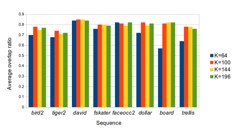
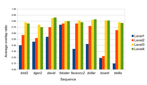
Generally, using larger dictionary and pooling more levels would improve classification accuracy, which however would inevitably lead to higher dimensional features. Thousands of dictionary bases are typically used in the image classification task. In the case of visual tracking, due to the real time limitation, the features can not be too high dimensional. Fortunately, the image patterns appeared in a tracking scene are relatively simple, which means that hundreds of dictionary words would be enough to yield good results. We thus evaluate four dictionary sizes (64, 100, 144, 196) as well as four pooling levels in terms of VOR scores in figure 3. It can be seen that using a dictionary of size 100 greatly promotes the performance on most of the sequences compared to size 64 except the faceocc2. Further enlarging it does not gain any significant improvement or even deteriorate the performance. As for the pooling levels, using more layers improves the tracking accuracy on most of the sequences. However, the difference gets less notable with the increase of the pooling levels except on the board sequence where the tracker with two-level pooling features lost the target. When the pooling level increases to 4, the performance even get worse due to overfitting. Based on these observations, we choose a dictionary size of 100 and 3-level pooling as a compromise for accuracy and efficiency to report the tracking results in Table 1 and 2.

Figure 3: Performance comparison of VOR scores with different dictionary sizes (top) and different pooling levels (bottom).

Comparing with other features in Struck

To further demonstrate the strength of the learned features, we incorporate the feature learning into the Struck framework and compare with three other types of features originally used in [2], which are raw pixel, Haar and histogram features. Linear kernel is used here for evaluation. All the other settings are the same with [2] for all the sequences. Table 6 reports the average VORs and CLEs on eight sequences. As can be can be observed, different hand-crafted features perform well in particular scenarios as they capture different information of the tracking scene, while as the learned feature achieves the overall best performance and outperforms its counterparts significantly. In conclusion, the features learned in a principled fashion is superior than the traditional hand-crafted features in tracking tasks.

Sequence	ST		Raw		Haar		Histogram
	VOR	CLE	VOR	CLE	VOR	CLE	VOR	CLE
david	0.82	7.1	0.38	51.3	0.46	45.5	0.70	14.3
girl	0.78	12.2	0.75	13.8	0.80	10.4	0.28	67.4
faceocc1	0.81	11.4	0.82	11.0	0.84	9.5	0.79	13.1
faceocc2	0.79	6.9	0.75	12.2	0.81	9.4	0.68	16.6
coke11	0.75	4.3	0.66	6.5	0.64	6.5	0.56	9.7
tiger1	0.76	4.9	0.68	7.6	0.32	37.7	0.72	5.6
tiger2	0.71	6.4	0.48	11.6	0.56	13.2	0.61	9.4
sylvester	0.77	7.0	0.69	9.2	0.62	11.7	0.76	6.8
average	0.77	7.5	0.65	15.4	0.63	18.0	0.64	17.9

Table 6: Performance comparison (VORs and CLEs) of different features using Struck with linear kernel. The last row shows the averaged results over all sequences. The best results are bold faced.

4.3 Discussions on dictionary update

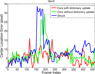
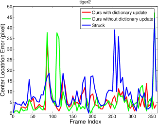
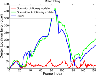
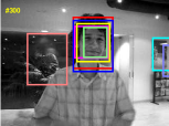
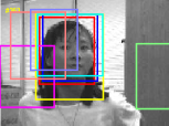
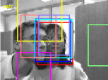
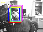
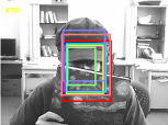
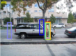
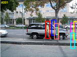
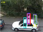
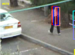
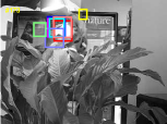
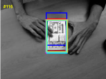
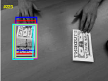
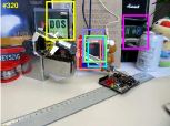
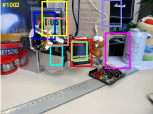
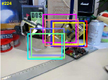
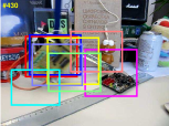
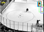
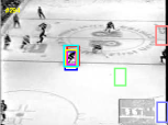
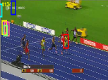
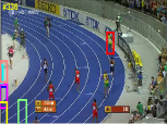
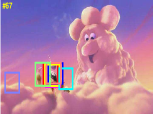
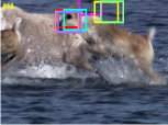
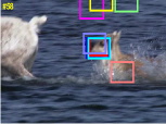
From the reported results, we can see that using the dictionary simply learned from the patches extracted in the first frame yields surprisingly satisfactory results, almost as good as its counterpart with updating scheme. We conjecture that this advantage comes from the fact that most of the tracking sequences consists of relatively simple patterns. Even with various changes, the scenes are similar. To demonstrate the effectiveness of the dictionary update scheme proposed here, we find a sequence with drastic scene changes as well as $360^{\circ}$ in-plane rotation of the object, which is motorRolling. Without update, our tracker lost the target at the frame 38 and yield a final VOR of 0.11 with the CLE 160.3. While equipped with the dictionary updating scheme, it tracks the target during the whole process giving an average VOR of 0.49 with the CLE 24.9, although not accurate enough due to the severe variations of the object appearance. Figure 4 shows the center location error plots of our method both with and without dictionary update compared to Struck on four sequences.

Figure 4: The center location error plots of our tracker with and without dictionary update compared with Struck on four sequences.

Figure 5: Qualitative comparison on sequence david, girl, faceocc2, david3, woman, tiger2, dollar, box, board, shaking, fskater, iceball, bolt, bird, deer.

5 Conclusion

We have presented an online feature learning based tracker in this work. The proposed tracker follows the classical feature learning pipeline, which consists of dictionary learning, feature encoding and spatial pooling. The online dictionary learning method is applied to account for the appearance variations of the tracking target. We also evaluate the roles of several commonly used dictionary learning as well as encoding approaches in the proposed tracking framework, and achieve similar conclusions with previous studies on image classification. When combined with Struck, the learned features help improve the tracking accuracy compared to traditional hand-crafted features. Experimental results on various challenging videos demonstrate that the proposed tracker outperforms the state-of-the-art. Future work may take into consideration incorporating motion models of the target and tracking multiple objects.

References

- [1] C. Bao, Y. Wu, H. Ling, and H. Ji, “Real time robust l1 tracker using accelerated proximal gradient approach,” in Proc. IEEE Conf. Comp. Vis. Patt. Recogn., 2012, pp. 1830–1837.
- [2] S. Hare, A. Saffari, and P. H. S. Torr, “Struck: Structured output tracking with kernels,” in Proc. IEEE Int. Conf. Comp. Vis., 2011.
- [3] L. Zhang and L. van der Maaten, “Structure preserving object tracking,” in Proc. IEEE Conf. Comp. Vis. Patt. Recogn., 2013.
- [4] X. Li, C. Shen, A. Dick, and A. van den Hengel, “Learning compact binary codes for visual tracking,” in Proc. IEEE Conf. Comp. Vis. Patt. Recogn., 2013.
- [5] R. Yao, Q. Shi, C. Shen, Y. Zhang, and A. van den Hengel, “Part-based visual tracking with online latent structural learning,” in Proc. IEEE Conf. Comp. Vis. Patt. Recogn., 2013.
- [6] S. Avidan, “Support vector tracking,” IEEE Trans. Pattern Anal. Mach. Intell., vol. 26, no. 8, pp. 1064–1072, 2004.
- [7] R. Yao, Q. Shi, C. Shen, Y. Zhang, and A. van den Hengel, “Robust tracking with weighted online structured learning,” in European Conf. Comp. Vis., 2012, vol. 7574, pp. 158–172.
- [8] H. Li, C. Shen, and Q. Shi, “Real-time visual tracking using compressive sensing,” in Proc. IEEE Conf. Comp. Vis. Patt. Recogn., June 2011, pp. 1305–1312.
- [9] Y. Wu, J. Lim, and M.-H. Yang, “Online object tracking: A benchmark,” in Proc. IEEE Conf. Comp. Vis. Patt. Recogn., 2013.
- [10] D. A. Ross, J. Lim, R.-S. Lin, and M.-H. Yang, “Incremental learning for robust visual tracking,” Int. J. Comp. Vis., vol. 77, no. 1-3, pp. 125–141, 2008.
- [11] X. Jia, H. Lu, and M.-H. Yang, “Visual tracking via adaptive structural local sparse appearance model,” in Proc. IEEE Conf. Comp. Vis. Patt. Recogn., 2012, pp. 1822–1829.
- [12] W. Zhong, H. Lu, and M.-H. Yang, “Robust object tracking via sparsity-based collaborative model,” in Proc. IEEE Conf. Comp. Vis. Patt. Recogn., 2012, pp. 1838–1845.
- [13] T. Zhang, B. Ghanem, S. Liu, and N. Ahuja, “Robust visual tracking via multi-task sparse learning,” in Proc. IEEE Conf. Comp. Vis. Patt. Recogn., 2012, pp. 2042–2049.
- [14] L. Sevilla-Lara and E. G. Learned-Miller, “Distribution fields for tracking,” in Proc. IEEE Conf. Comp. Vis. Patt. Recogn., 2012, pp. 1910–1917.
- [15] S. Avidan, “Ensemble tracking,” IEEE Trans. Pattern Anal. Mach. Intell., vol. 29, no. 2, pp. 261–271, Feb. 2007.
- [16] B. Babenko, M.-H. Yang, and S. J. Belongie, “Visual tracking with online multiple instance learning,” in Proc. IEEE Conf. Comp. Vis. Patt. Recogn., 2009, pp. 983–990.
- [17] Z. Kalal, J. Matas, and K. Mikolajczyk, “P-N learning: Bootstrapping binary classifiers by structural constraints,” in Proc. IEEE Conf. Comp. Vis. Patt. Recogn., 2010, pp. 49–56.
- [18] A. Coates, A. Y. Ng, and H. Lee, “An analysis of single-layer networks in unsupervised feature learning,” Proc. Int. Conf. Artificial Intell. & Stat., vol. 15, pp. 215–223, 2011.
- [19] A. Coates and A. Y. Ng, “The importance of encoding versus training with sparse coding and vector quantization,” in Proc. Int. Conf. Mach. Learn., 2011, pp. 921–928.
- [20] Y. Jia, C. Huang, and T. Darrell, “Beyond spatial pyramids: Receptive field learning for pooled image features,” in Proc. IEEE Conf. Comp. Vis. Patt. Recogn., 2012, pp. 3370–3377.
- [21] K. Sohn, D. Y. Jung, H. Lee, and A. O. Hero, “Efficient learning of sparse, distributed, convolutional feature representations for object recognition,” in Proc. IEEE Int. Conf. Comp. Vis., 2011, pp. 2643–2650.
- [22] A. Shabou and H. L. Borgne, “Locality-constrained and spatially regularized coding for scene categorization,” in Proc. IEEE Conf. Comp. Vis. Patt. Recogn., 2012, pp. 3618–3625.
- [23] M. Aharon, M. Elad, and A. Bruckstein, “K-SVD: An algorithm for designing overcomplete dictionaries for sparse representation,” IEEE Trans. Signal Process., vol. 54, no. 11, pp. 4311–4322, Nov. 2006.
- [24] J. Wang, J. Yang, K. Yu, F. Lv, T. Huang, and Y. Gong, “Locality-constrained linear coding for image classification,” in Proc. IEEE Conf. Comp. Vis. Patt. Recogn., 2010.
- [25] J. Mairal, F. Bach, J. Ponce, and G. Sapiro, “Online learning for matrix factorization and sparse coding,” J. Mach. Learn. Res., vol. 11, pp. 19–60, 2010.
- [26] F. Tang, S. Brennan, Q. Zhao, and H. Tao, “Co-tracking using semi-supervised support vector machines,” in Proc. IEEE Conf. Comp. Vis. Patt. Recogn., 2007, pp. 1–8.
- [27] X. Mei and H. Ling, “Robust visual tracking and vehicle classification via sparse representation,” IEEE Trans. Pattern Anal. Mach. Intell., vol. 33, no. 11, pp. 2259–2272, Nov. 2011.
- [28] Q. Wang, F. Chen, J. Yang, W. Xu, and M.-H. Yang, “Transferring visual prior for online object tracking,” IEEE Trans. Image Proc., vol. 21, no. 7, pp. 3296–3305, 2012.
- [29] B. Liu, J. Huang, L. Yang, and C. Kulikowsk, “Robust tracking using local sparse appearance model and k-selection,” in Proc. IEEE Conf. Comp. Vis. Patt. Recogn., 2011, pp. 1313–1320.
- [30] Y.-L. Boureau, F. Bach, Y. LeCun, and J. Ponce, “Learning mid-level features for recognition,” in Proc. IEEE Conf. Comp. Vis. Patt. Recogn., 2010, pp. 2559–2566.
- [31] B. Efron, T. Hastie, I. Johnstone, and R. Tibshirani, “Least angle regression,” Annals of Statistics, vol. 32, pp. 407–499, 2004.
- [32] J. Ye and T. Xiong, “SVM versus least squares svm.,” Proc. Int. Conf. Artificial Intell. & Stat., vol. 2, 2007.
- [33] L. Liu, L. Wang, and X. Liu, “In defense of soft-assignment coding,” in Proc. IEEE Int. Conf. Comp. Vis., 2011, pp. 2486–2493.