Transmit Beamforming for MIMO Communication Systems with Low Precision ADC at the Receiver

Abstract

Multiple antenna systems have been extensively used by standards designing multi-gigabit communication systems operating in bandwidth of several GHz. In this paper, we study the use of transmitter (Tx) beamforming techniques to improve the performance of a MIMO system with a low precision ADC. We motivate an approach to use eigenmode transmit beamforming (which imposes a diagonal structure in the complete MIMO system) and use an eigenmode power allocation which minimizes the uncoded BER of the finite precision system. Although we cannot guarantee optimality of this approach, we observe that even low with precision ADC, it performs comparably to full precision system with no eigenmode power allocation. For example, in a high throughput MIMO system with a finite precision ADC at the receiver, simulation results show that for a $\frac{3}{4}$ LDPC coded $2\times 2$ MIMO OFDM 16-QAM system with 3-bit precision ADC at the receiver, a BER of $10^{-4}$ is achieved at an SNR of $26$ dB. This is $1$ dB better than that required for the same system with full precision but equal eigenmode power allocation.

I Introduction

Several standards designing muliGigabit communication systems (for example, IEEE 802.11ad and IEEE 802.15.3c) use multiple antennas at both the transmitter and receiver to boost up the data rates in the range of several Gbps. This gives rise to multiple input multiple output (MIMO) channel configurations. Almost all communication system with MIMO channels implement their receiver operations in the digital domain and thus analog to digital converters (ADC) becomes a critical component for such systems. Most communication system use ADCs with a precision of 6–8 bits per sample. However, high precision ADCs operating at sampling rates of several giga-samples-per second are extremely power hungry and expensive ([1, 2, 3]). Consequently, for designing communication systems requiring such high speed sampling, ADC becomes a bottleneck. We would like to highlight that a similar problem does exist for digital-to-analog (DAC) conversion (DAC) at the transmitter. However, we assume that the transmitter has significantly more power resources compared to the receiver and we focus only on the ADC problem. An example of such a scenario is when a handheld device downloads high definition content from an access point but uploads at normal speeds.

A naive method to reduce the power consumption at the receiver is to use an ADC with a low bit precision (1-4 bits per sample). However, this can lead to serious performance degradation (see Fig. 2). In the remainder of this section, we survey some of the previous works and highlight our contribution to improve the performance of a MIMO communication system when a low bit precision ADC is used at the receiver. We also set down some notational conventions at the end of this section.

I-A Prior Work

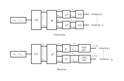
Figure 1: System block diagram for MIMO OFDM with Tx-Rx beamforming.

Recently, there has been significant effort to address the ADC bottleneck and implement receivers for multi-Gbps single input single output (SISO) communication systems using low precision ADC at the receivers. Typically in SISO OFDM systems, equal transmit power subcarrier (ETSP) power is used. However, due to wide channel gain variations across the subcarriers, use of low precision ADC at the receiver results in loss of information from the weak carriers. As a result, the inter-carrier interference is not be canceled and we get an error floor (see Fig. 1 in [4]). In [4], we suggest a transmitter based technique for subcarrier interference management using subcarrier power allocation to ameliorate the error floor. In [5], we further extend this work to find an optimal power allocation to minimize the error at the receiver. Using this optimal scheme, we observe that using a $3$–bit precision ADC at the receiver of $\frac{7}{8}$ LDPC coded $16$–QAM OFDM system, we can achieve a $2$ dB improvement in the performance compared to ETSP based OFDM. In this paper, we extend our earlier work to MIMO OFDM system.

There is considerable literature in the design of transmitter-receiver (Tx-Rx) beamforming (joint or otherwise) techniques which optimizes a certain performance metric like mean square error (MSE), signal-to-interference noise ration (SINR), bit error rate (BER), transmit power etc. (see for example [6, 7, 8, 9] and references therein) for full precision MIMO receivers. However, to the best of our knowledge, there has been no work in the design of Tx-Rx beamformers for MIMO receivers for a finite precision ADC.

In this paper, using ideas similar to the use of sub-carrier power allocation for OFDM systems to improve the performance of a low precision receiver ([4], [5]), we use Tx-beamforming methods to achieve full precision performance for a MIMO receiver with a low precision ADC.

I-B Our Contribution

Exact expressions for BER for finite precision MIMO systems are fairly complicated and not amenable to finding closed form expression or computationally efficient algorithms for optimal Tx-beamformers. Instead, we impose a specific structure on the Tx-beamformer which transmits on the eigenmodes and diagonalizes the overall system. Although the optimality of diagonalization property cannot be proved in general for a BER minimization criteria, we motivate this property from the existence of similar property for MSE minimization criteria. This greatly simplifies the optimization problem and reduces it to a eigenmode power allocation problem.

For such a diagonal structure, we compute exact expression for the uncoded BER of the MIMO-OFDM system with finite precision ADC at the receiver (Proposition 1, part 1). Using this expression of uncoded BER, we obtain a eigenmode power allocation (OEPA) which minimizes it (Proposition 1, part 2). We also propose a useful closed form approximately optimal eigenmode power allocation (27) which can be easily used in practical system without significant increase in computational or storage requirements. We use simulations to illustrate the improvement in the performance using our power allocation stream with a low precision ADC at the receiver. As suggested in [10], we use the Saleh Valenzuela (SV) to model the channel. We find that for a $\frac{3}{4}$ LDPC coded $2\times 2$ MIMO OFDM 16-QAM system with 3-bit precision at the receiver, our method requires $1$ dB less power compared to the traditional full precision system with equal eigenmode power allocation (EEPA) to achieve a BER of $10^{-4}$. On the other hand, a 3-bit system with EEPA has an error floor of $10^{-2}$.

I-C Notation

We use small case bold face letter to represent vectors and small case italics letters to represent scalars. Upper case bold face letter are used to represent matrices. The superscripts $[\cdot]^{\dagger}$ and $[\cdot]^{T}$ are used to denote conjugate transpose and transpose, respectively. We use $\mathbf{X}=\text{diag}\left(\mathbf{X}_{1}\ldots\mathbf{X}_{L}\right)$ to represent a block diagonal matrix where each block is $\mathbf{X}_{i}$, $1\leq i\leq L$. We use $\mathbf{I}$ to denote an identity matrix. The dimension of the identity matrix follows from the context.

II System Description

II-A MIMO Channel model

For each single input single output channel between transmit antenna $i$ and receive antenna $j$, we consider an independent ISI channel in which the resolved multipath components are grouped into $L_{c}$ clusters, each having $L_{b}$ rays. The time domain channel impulse response is given by

$$h(t)=\sum_{c=0}^{H_{c}-1}\sum_{b=0}^{H_{b}-1}g_{c,b}\delta\left(t-T_{c}-\tau_{c,b}\right),$$ (1)

where $g_{c,b}$ is the tap weight of the $b$-th ray of the $c$-th cluster, $T_{c}$ is the delay of $c$-th cluster, $\tau_{c,b}$ is the delay of the $b$-th ray relative to $T_{c}$ and $\delta(\cdot)$ is the dirac delta function. For simplicity of notation, we do not show the dependence on $i$ and $j$. Most standards like IEEE 802.15.3c which design communication system over a wideband channel, the Saleh-Valenzuela (S-V) model is the most popular model which characterizes the statistical properties of the parameters in (1). According to this model,

$$f\left(T_{c}|T_{c-1}\right) =\Lambda\exp\left[-\Lambda\left(T_{c}-T_{c-1}\right)\right],\quad c>0$$ (2)

$$f\left(\tau_{c,b}|\tau_{c,\left(b-1\right)}\right) =\lambda\exp\left[-\lambda\left(\tau_{c,b}-\tau_{c,\left(b-1\right)}\right)\right],\quad b>0$$ (3)

where $\Lambda$ and $\lambda$ are the cluster and ray arrival rate, respectively, and $f(\cdot)$ is the probability density function. Also, the mean square power of the tap weights are

$$\text{E}[|g_{c,b}|^{2}]=\text{E}[|g_{0,0}|^{2}]\exp\left(-\frac{T_{c}}{\Gamma}\right)\exp\left(-\frac{\tau_{c,b}}{\gamma}\right),$$ (4)

where $\Gamma$ and $\gamma$ are the cluster and ray decay rates, respectively. Since we are in the wideband regime, the distribution of the channel taps is modeled by a lognormal distribution [11, 12].

The receiver implements a front end filter of sufficient bandwidth and then samples the received analog signal uniformly. We assume that all the channel response vectors have length $L$

II-B Signal model for a MIMO-OFDM channel with a finite precision receiver

We consider a communications system with $n_{T}$ transmit antennas and $n_{R}$ receiver antennas which gives rise to a MIMO channel. In case of flat faded channels, the MIMO channel is represented by a channel matrix, where any entry $(i,j)$ of the matrix is channel gain between antenna $i$ and antenna $j$. In case of MIMO frequency selective channel, a multicarrier scheme is often used and each transmit antenna has an OFDM modulator and each receiver antenna has an OFDM demodulator (this can be assumed without any loss in capacity as showed in [9, 13]). A detailed explanation of single input single output (SISO) OFDM can be found in [14] and we omit several details details here.

Let $\mathbf{u}_{i}\in\mathbb{C}^{N\times 1}$ be the frequency domain vector to be transmitted at antenna $i$. Define $\mathbf{u}:=\left[\mathbf{u}_{1}\ldots\mathbf{u}_{n_{T}}\right]^{T}$ and $L:=\min(n_{T},n_{R})$. We assume a carrier–cooperative Tx–beamformer $\mathbf{B}\in\mathbb{C}^{n_{T}N\times LN}$ which allows for cooperation between different subcarriers while designing $\mathbf{B}$. The vector $\mathbf{u}$ is given by

$$\mathbf{u}=\mathbf{B}\mathbf{x},$$ (5)

where $\mathbf{x}=\left[\mathbf{x}_{1}^{T}\ldots\mathbf{x}_{L}^{T}\right]^{T}\in\mathbb{C}^{LN}$ is the data vector to be communicated. We assume w.l.o.g. $\text{E}[\mathbf{x}\mathbf{x}^{\dagger}]=\mathbf{I}$. Let $\mathbf{F}$ be a block diagonal matrix of size $Nn_{T}\times Nn_{T}$ where each block is the N-point discrete Fourier matrix $\mathbf{F_{N}}$. The time domain transmitted vector from any antenna $i$ is given by

$$\mathbf{s}_{i}=\mathbf{F}^{\dagger}_{N}\mathbf{u}_{i}.$$ (6)

Thus we can define a vector $\mathbf{s}:=\left[\mathbf{s}_{1}^{T}\ldots\mathbf{s}_{n_{T}}^{T}\right]^{T}=\mathbf{F}^{\dagger}\mathbf{u}$. The total power constraint at transmitter can be expressed as

$$\text{E}\left[||\mathbf{s}||^{2}\right]=Tr\left(\mathbf{B}^{\dagger}\mathbf{B}\right)\leq NL.$$ (7)

At the receiver, the analog samples are down converted and discretized. If the discretization is done at full precision, the received vector $\mathbf{r}_{j}\in\mathbb{C}^{N}$ (after removing the cyclic prefix) is given by

$$\mathbf{r}_{j}=\mathbf{C}_{j}\mathbf{s}+\mathbf{w}_{j},$$ (8)

where $\mathbf{w}_{j}$ is additive zero mean Gaussian noise with covariance matrix $\xi^{2}\mathbf{I}$ and we define $\mathbf{C}_{j}:=[\mathbf{C}_{j,1}\ldots\mathbf{C}_{j,n_{T}}]$ and $\mathbf{C}_{j,i}$ represents the time domain SISO channel between transmit antenna $i$ and receive antenna $j$. The construction of the OFDM symbol forces the matrix $\mathbf{C}_{i,j}$ to be a circulant matrix. However, in practical systems, the discretization is done with finite precision. Let $A(\cdot)$ be the map which represents the analog-to-digital conversion. The ADC is defined by two parameters.

$Resolution$ $b$: If the resolution is $b$ bits, then the real and imaginary parts are each quantized to $2^{b}$ levels.

$Range$: We assume that $A(\cdot)$ has a constant range of $(-1,+1)$. If the sampled signal exceeds this range, then it is clipped. In practice, an AGC block, with gain $G$ is used prior to the quantization to ensure that clipping occurs with low probability. In all our simulations, we use a uniform mid-point quantizer with range $(-1,1)$ and resolution $b$:

$$\begin{split}A(x)&=\text{sign}\left(x\right)\left(\frac{1}{2^{b-1}}\lfloor 2^{b-1}|x|\rfloor+\frac{1}{2^{b}}\right),\quad|x|\leq 1.\\ &=\text{sign}\left(x\right)\left(1-\frac{1}{2^{b}}\right),\quad\text{otherwise}.\end{split}$$ (9)

where $\lfloor z\rfloor$ is the largest integer lesser than $z$. Then the received vector (after removing the cyclic prefix) at antenna $j$ is given by $\mathbf{r}^{q}_{j}=A\left(\mathbf{C}_{j}\mathbf{s}+\mathbf{w}_{j}\right),$where $A(\cdot)$ is applied elementwise. Defining $\mathbf{r}^{q}:=\left[\mathbf{r}^{q^{T}}_{1}\ldots\mathbf{r}^{q^{T}}_{n_{R}}\right]^{T}$, and $\mathbf{w}:=\left[\mathbf{w}^{T}_{1}\ldots\mathbf{w}^{T}_{n_{R}}\right]^{T}$ $\mathbf{C}=\left[\mathbf{C}_{1}\ldots\mathbf{C}_{n_{R}}\right]^{T}$, we can write

$$\mathbf{r}^{q}=A\left(\mathbf{C}\mathbf{s}+\mathbf{w}\right)$$ (10)

Modeling quantization noise: Due to the quantizer nonlinearity, analyzing an OFDM system with finite precision quantization becomes intractable. A simple heuristic is to model the quantization noise as additive and independent (see pseudo quantization noise model in Chapter 4 of [15]). It is shown in [16] that the PQN model is a valid model for quantization of OFDM signal only for a certain range of AGC. A description of the AGC calibration to ensure that the PQN model is valid is explained in [5]. As per this description, if

$$G^{2}=\frac{Nn_{R}\alpha}{\text{E}[||\mathbf{r}||^{2}]},$$ (11)

for a suitably chosen $\alpha$, where $\mathbf{r}=\left[\mathbf{r}_{1}^{T}\ldots\mathbf{r}_{n_{R}N}^{T}\right]^{T}$, the PQN model is a reasonable model for the quantization error.

Using this model for quantization error, we can write

$$\mathbf{r}^{q}_{j}=\mathbf{C}_{j}\mathbf{s}+\mathbf{w}_{j}+\mathbf{q}_{j}.$$ (12)

where $\mathbf{q}_{j}\in\mathbb{C}^{N\times 1}$ is the additive zero mean uniformly distributed quantization noise with covariance matrix $\frac{1}{G^{2}}\frac{2^{-2b}}{6}\mathbf{I}$. The receiver further transforms the received vector into the frequency domain by applying a $N$-point DFT,

$$\mathbf{v}_{j}=\mathbf{F}_{N}\mathbf{r}^{q}_{j}.$$ (13)

Combining (5), (6) and (12) along with the fact that $\mathbf{D}_{ji}:=\mathbf{F}_{N}\mathbf{C}_{ji}\mathbf{F}_{N}^{\dagger}$ is a diagonal matrix, we get

$$\mathbf{v}_{j}=\mathbf{D}_{j}\mathbf{Bx}+\mathbf{F}_{N}\mathbf{w}_{j}+\mathbf{F}_{N}\mathbf{q}_{j},$$ (14)

where $\mathbf{D}_{j}=\left[\mathbf{D}_{j1}\ldots\mathbf{D}_{jn_{T}}\right]$. Concatenating the frequency domain vectors from all $n_{R}$ antennas, we can write

$$\mathbf{v}=\mathbf{DBx}+\mathbf{Fw}+\mathbf{Fq},$$ (15)

where $\mathbf{D}:=\left[\mathbf{D}_{1}\ldots\mathbf{D}_{n_{R}}\right]^{T}$, $\mathbf{v}:=\left[\mathbf{v}^{T}_{1}\ldots\mathbf{v}^{T}_{n_{R}}\right]^{T}$ and $\mathbf{q}:=\left[\mathbf{q}^{T}_{1}\ldots\mathbf{q}^{T}_{n_{R}}\right]^{T}$. Let $\mathbf{A}$ be the Rx-beamformer. Again assuming cooperation among different carriers, the vector $\mathbf{v}$ is linearly transformed as

$$\hat{\mathbf{x}}=\mathbf{A}^{\dagger}\mathbf{v}=\mathbf{A}^{\dagger}\mathbf{DBx}+\mathbf{A}^{\dagger}\mathbf{Fw}+\mathbf{A}^{\dagger}\mathbf{Fq}.$$ (16)

The statistic $\hat{\mathbf{x}}$ is used as a statistic to decode the data vector $\mathbf{x}$.

III Optimal Tx-beamforming for MIMO systems for a specified Rx-beamformer

Often in downlink systems where the receivers have limited resources, it is beneficial to have a pre-specified linear receivers which depend only on the channel and not on the Tx-beamformer. For such systems systems, the goal is to design Tx-beamformers which optimizes a suitable metric. For most communication systems, the ultimate metric which we desire to optimize is the bit error rate. For the MIMO system (16) with $\hat{L}=\min\left(L,\text{rank}\left(D^{\dagger}D\right)\right)$ substreams, the average BER can be defined as

$$\text{BER}=\frac{1}{\hat{L}}\sum_{l=1}^{\hat{L}}\text{BER}_{l}$$ (17)

where $\text{BER}_{l}$ is the bit error rate for the $l$th substream. For a M-QAM constellation, a first order approximation of $\text{BER}_{l}$ can be expressed as a function of the expected signal-to-interference noise ratio (SINR) on the $l$th substream as

$$\text{BER}_{l}\approx\frac{1}{\log_{2}M}\left(1-\frac{1}{\sqrt{M}}\right)Q\left(g_{M}\text{SINR}_{l}\right).$$ (18)

where $g_{M}=\frac{3}{M-1}$ and $Q(\cdot)$ is the tail probability of normal random distribution ([8]). Using (16), we can write

$$\text{SINR}_{l}=\frac{|\mathbf{a}_{l}^{\dagger}\mathbf{Db}_{l}|^{2}}{\mathbf{a}^{\dagger}_{l}\left(\xi^{2}\mathbf{I}+\xi_{q}^{2}\mathbf{I}+\sum_{k\neq l}\mathbf{Db}_{k}\mathbf{b}_{k}^{\dagger}\mathbf{D}^{\dagger}\right)\mathbf{a}_{l}}$$ (19)

where $\xi_{q}^{2}=\frac{1}{G^{2}}\frac{2^{-2b}}{6}$ and $\mathbf{b}_{l}$ and $\mathbf{a}_{l}$ are the $l$th column vectors of $\mathbf{A}$ and $\mathbf{B}$, respectively. Thus a BER minimizing criteria to design the Tx-beamformer can be written as

$$\begin{split}\min_{\hat{\mathbf{B}}\in\mathbb{C}^{LN\times Nn_{T}}}\text{BER},\quad\text{subject to}\\ Tr\left(\hat{\mathbf{B}}^{\dagger}\hat{\mathbf{B}}\right)\leq NL.\end{split}$$ (20)

A standard method to solve such problems is to use the Lagrange multiplier method. However, this method does not provide any closed form solution to compute $\mathbf{B}$. Instead a set of matrix fixed point equations are obtained, the solution of which is difficult to compute over a large search space. In view of the space constraints, we do not write down this equations in this draft. For example, in a $2\times 2$ MIMO OFDM system with $128$ sub-carriers, we have $256\times 256$ variables to be optimized. For full precision systems, several techniques have been used to get around the intractability of BER expressions e.g. using Chernoff bounds for the $Q(\cdot)$ function or maximizing the minimum of the SINR over all substreams. One other popularly used method is to minimize the mean square error (MSE) between $\mathbf{x}$ and $\hat{\mathbf{x}}$. We would like to point out that there exists a explicit analytical relationship between SINR and MSE only when optimal Weiner filters are used as beamformers at the receiver. Therefore, maximizing the SINR is equivalent to minimizing the MSE only for jointly designing Tx-Rx beamformers. Although this techniques do not necessarily guarantee a closed form expression for the optimal Tx-beamformer, it often helps in designing simpler algorithms. As representative example, we explain one such method which minimizes the MSE.

Minimizing the MSE criteria: From (16), the MSE can be expressed as

$$\text{MSE}=\text{E}\left[\|\mathbf{x}-\hat{\mathbf{x}}\|^{2}\right]=\|\mathbf{A}^{\dagger}\mathbf{DB}-\mathbf{I}\|^{2}_{F}+\left(\xi^{2}+\xi_{q}^{2}\right)\|\mathbf{A}\|_{F}^{2},$$ (21)

where $\|\cdot\|_{F}$ denotes the Frobenius norm. For the moment we consider the full precision case i.e. $\xi_{q}^{2}=0$. Then, if the channel is perfectly known at the receiver and the transmitter, the design criteria to find the optimal $\mathbf{B}$ is

$$\begin{split}\min_{\hat{\mathbf{B}}\in\mathbb{C}^{Nn_{T}\times NL}}&\|\mathbf{A}^{\dagger}\mathbf{DB}-\mathbf{I}\|^{2}_{F},\quad\text{subject to}\\ Tr\left(\hat{\mathbf{B}}^{\dagger}\hat{\mathbf{B}}\right)&\leq NL.\end{split}$$ (22)

Lemma 1:

Define $\bar{\mathbf{D}}:=\mathbf{A}^{\dagger}\mathbf{D}$. Let $\mathbf{U}_{\bar{D}}\mathbf{\Delta}_{\bar{D}}\mathbf{V}_{\bar{D}}^{\dagger}$ and $\mathbf{U}_{B}\mathbf{\Delta}_{B}\mathbf{V}_{B}^{\dagger}$ be the singular value decompositions of $\bar{\mathbf{D}}$ and $\mathbf{B}$, respectively. Then optimality (with respect to (23)) is achieved when $\mathbf{U}_{B}=\mathbf{V}_{\bar{D}}$ and $\mathbf{V}_{B}=\mathbf{U}_{\bar{D}}$.

This lemma is proved as a part of Theorem 1 in [17]. Consequently, this proves the optimality of eigen mode transmission and hence the optimality of the diagonal structure of the complete channel described by the matrix $\mathbf{A}^{\dagger}\mathbf{DB}$. This reduces the complicated matrix optimization problem into a scalar power allocation problem, where the diagonal elements of the matrix $\mathbf{\Delta}_{B}$ gives the power allocated on the eigen modes. Using the above proposition, the optimization problem in (23) simplifies to

$$\begin{split}\min_{\Delta_{B,1},\ldots,\Delta_{B,NL}}&\sum_{l=1}^{NL}\left(\Delta_{B,l}\Delta_{\bar{D},l}-1\right)^{2},\quad\text{subject to}\\ \sum_{l=1}^{NL}\Delta_{B,l}^{2}&\leq NL,\end{split}$$ (23)

where $\{\Delta_{B,l}\}$ and $\{\Delta_{\bar{D},l}\}$ are the diagonal elements of $\mathbf{\Delta}_{B}$ and $\mathbf{\Delta}_{\bar{D}}$, respectively.

IV A simpler approach to design Tx-beamformers using the BER critieria

As proved in Lemma 1, the diagonal structure is optimal while using minimum MSE as the criterion for designing TX-beamformers for pre-specified Rx-beamformers. This simplification of the problem makes it more amenable for obtaining closed form approximations or designing faster algorithms. However, there does not exist a general optimality of diagonalization result for the BER or SINR criteria (diagonalization is optimal only when the Rx-beamformer is an optimal Weiner filter). Instead to utilize the useful properties of the diagonal structure, we suggest the following heuristic approach to design Tx-beamformers.

1. For the specified linear Rx-beamformer $\mathbf{A}$, find the Tx-beamformer such that $\mathbf{A}^{\dagger}\mathbf{DB}$ is diagonalized (as suggested in Lemma 1).

2. Use this diagonal structure to obtain an expression of the average BER (which is the average of BER on each parallel sub-channel).

3. Compute the optimal eigen mode power allocation by minimizing the average BER.

As an example of the application of this approach, we consider a MIMO system where $\mathbf{A}=\mathbf{V}_{D}$ and $\mathbf{U}_{D}\mathbf{\Delta}_{D}\mathbf{V}_{D}$ is the singular value decomposition (SVD) of $\mathbf{D}$. According to part 1) of the method described above, we can use Lemma 1 to impose a diagonal structure on the complete MIMO system. This gives $\mathbf{B}=\sqrt{\mathbf{P}}\mathbf{U}_{D}$ where $\sqrt{\mathbf{P}}=\text{diag}\left(\sqrt{P_{1}}\ldots\sqrt{P_{NL}}\right)$ is the eigen power allocation to be determined. Such SVD based systems are often used in very high throughput systems (which is the main motivation of our work) which try to maximize the multiplexing gain. Without loss of generality, we assume all the singular values of $\mathbf{D}$ to be positive (If the matrix $\mathbf{D}$ has singular values to be zero, we remove that parallel channel from the system model). Since $\mathbf{U}_{D}$ is unitary, the power constraint (7) is satisfied if $\text{Tr}\left(\mathbf{P}\right)\leq NL$. Under this structural assumptions, (16) can be written as

$$\hat{\mathbf{x}}=\mathbf{P}\mathbf{\Delta_{D}}\mathbf{x}+\bar{\mathbf{w}}+\bar{\mathbf{q}},$$ (24)

where $\bar{\mathbf{w}}=\mathbf{V}_{D}^{\dagger}\mathbf{Fw}$ and $\bar{\mathbf{q}}=\mathbf{V}_{D}^{\dagger}\mathbf{Fq}$. Since $\mathbf{V}$ and $\mathbf{F}$ are unitary, $\text{E}[\bar{\mathbf{w}}\bar{\mathbf{w}}^{\dagger}]=\xi^{2}\mathbf{I}$. Using the asymptotic normality results in [18], we can model $\bar{\mathbf{q}}$ to be a a zero mean Gaussian vector with covariance matrix $\xi_{q}^{2}\mathbf{I}$ , where $\xi_{q}^{2}=\frac{1}{G^{2}}\frac{2^{-2b}}{6}$. Using the model (24), we have the following proposition

Proposition 1:

Under the preceding assumptions, the following statement holds true

1. The uncoded BER for a $M-$QAM OFDM communication system with a $n_{T}\times n_{R}$ MIMO channel (parallelized into $L=\min(n_{T},n_{R})$ independent channels as described in the preceding discussion) and eigen power allocation $\mathbf{P}$ is given by

   $$BER=\frac{4S-O(S^{2})}{\log_{2}M}$$ (25)

   where

   $$\begin{split}S&=\left(1-\frac{1}{\sqrt{M}}\right)\frac{1}{LN}\\ &\times\sum_{k=1}^{LN}Q\left(\sqrt{g_{M}\frac{P_{k}|\Delta_{D,k}|^{2}}{(c+1)\xi^{2}+\xi_{q}^{2}}}\right),\end{split}$$

   $$\begin{split}g_{M}&=\frac{3}{M-1},c=\frac{2^{-2b}}{6\alpha}\\ \text{and }&\xi_{q}^{2}=c\left(\frac{1}{LN}\sum_{j=0}^{LN}P_{j}|\Delta_{D,j}|^{2}\right).\end{split}$$

   and $\{\Delta_{D,k}\}$ are the singular values of $\mathbf{D}$.

2. An optimal eigenmode power allocation $\mathbf{P}^{(b)}$ (OEPA) which minimizes $S$ defined in Part 1) is

   $$P_{k}^{(b)}=\frac{\left(\xi^{2}+\xi_{q}^{2}\right)W\left(\frac{g_{M}|\Delta_{D,k}|^{4}}{\left((c+1)\xi^{2}+\xi_{q}^{2}\right)^{2}\left(\Omega^{2}+|\Delta_{D,k}|^{2}a^{2}\right)}\right)}{g_{M}|\Delta_{D,k}|^{2}},$$ (26)

   where $W(\cdot)$ is the principal value Lambert function [19],

   $$a=c\sum_{j=1}^{LN}\frac{\sqrt{P^{(b)}_{j}|\Delta_{D,j}|^{2}}\exp\left(-\frac{g_{M}P_{j}^{b}|\xi_{j}|^{2}}{\xi^{2}+\xi_{q}^{2}}\right)}{\left(\xi^{2}+\xi_{q}^{2}\right)^{\frac{3}{2}}}$$

   and $\Omega$ is chosen to satisfy the power constraint (7). The Lambert function $W(\cdot)$ is defined as inverse function of $f(w)=w\exp(w).$

Discussion: The proof of part 1) and part 2) are on similar lines to the proof of part 1) and part 2) of Proposition 1 in [5]. Computing OEPA using (26) is computationally expensive and we propose the following approximate OEPA (AOEPA).

$$\tilde{P}_{k}^{(\infty)}=\frac{\frac{W\left(\frac{g_{M}|\Delta_{D,k}|^{4}}{\xi^{4}}\right)}{|\Delta_{D,k}|^{2}}}{\sum_{j=1}^{LN}\frac{W\left(\frac{g_{M}|\Delta_{D,j}|^{4}}{\xi^{4}}\right)}{|\Delta_{D,j}|^{2}}},\quad\forall k,$$ (27)

The motivation of the approximation follows from the discussion in Section III.C of [5].

Remark: The ultimate goal is to minimize coded BER but for analytical tractability we have worked with uncoded BER. In the next section, we show using simulations that the proposed power allocation also improves coded BER performance.

V Simulation Results

In this section, we present simulation results which highlights the improvement in the performance when using the Tx-Rx beamforming scheme presented in Section IV. For carrying out the simulations, the values of the parameters of the OFDM symbol and the MIMO channel model are summarized in Table I.

TABLE I: Parameter values used in the simulation.

Number of transmit antennas	$n_{T}$	$2$
Number of receive antennas	$n_{R}$	$2$
Name of parameter	Symbol	Value
Number of subcarriers	$N$	$512$
OFDM symbol duration	$T_{s}$	$204.8$ ns
Length of cyclic prefix	$L$	64
Cluster arrival rate	$\Lambda$	$0.037$ $ns^{-1}$
Ray arrival rate	$\lambda$	$0.641$ $ns^{-1}$
Cluster decay rate	$\Gamma$	$21.1$ $ns$
Ray decay rate	$\gamma$	$8.85$ $ns$
Cluster lognormal standard deviation	$\sigma_{c}$	$3.01$ dB
Ray lognormal standard deviation	$\sigma_{r}$	$7.69$ dB
Mean number of clusters	$L_{c}$	$3$
Mean number of rays	$L_{r}$	$5$

We consider a high throughput $2\times 2$ MIMO system communication system which is parallelized using SVD described in previous section We highlight four possible scenarios for such a system: 1) EEPA with full precision ADC, 2) EEPA with a 3-bit precision ADC, 3) MSE minimizing eigenmode power allocation (which we call MMSE-PA) obtained by solving (23) with a 3-bit precision ADC, and 4) AOEPA given by (27) with 3-bit precision ADC. From Fig. 2, we see that for a $\frac{3}{4}$-rate low density parity check code (LDPC) coded $2\times 2$ MIMO OFDM system with 3-bit receiver, AOEPA achieves a BER of $10^{-4}$ at an SNR of $26$ dB compared to $27$ dB required with full precision with EEPA. On the other hand, a 3-bit system with EEPA requires has an error floor of $10^{-2}$. Similarly from Fig. 3, for a $\frac{1}{2}$-rate $2\times 2$ MIMO OFDM system, 3-bit AOEPA requires $1$ dB less power than EEPA full precision system.

The comparison of MSE minimizing eigen mode power allocation (MMSE-PA) with AOEPA provides a justification for our method. Even though the MSE criteria has the optimality of diagonalization property while BER criteria is not guaranteed of such property, optimal eigenmode power allocation which minimizes the MSE performs worse (it requires 30 dB to achieve BER of $10^{-4}$) compared to AOEPA. This justifies our approach to impose a diagonalizing structure on the MIMO system, computing the average BER (which is easier to calculate) and thereafter computing the eigenmode power allocations which minimize the BER.

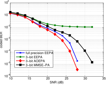
Figure 2: Coded BER performance for a rate $\frac{3}{4}-$rate LDPC coded $2\times 2$ high throughput MIMO OFDM system for EEPA, AOEPA and MMSE-PA.

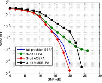
Figure 3: Coded BER performance for a rate $\frac{1}{2}-$rate LDPC coded $2\times 2$ high throughput MIMO OFDM system for EEPA, AOEPA and MMSE-PA.

VI Conclusion

In this paper, we investigate a Tx beamforming approach to improve performance of a MIMO-OFDM system with a low precision ADC at the receiver. We use Lemma 1 as a motivation and impose the structure emerging out of it to find a Tx-beamformer which minimizes the BER criteria. The primary reason for imposing this structure is reduction of the dimensionality of the space we are optimizing over. Due to this structure, the beamformer transmits on the eigenmodes of the channel and power allocation on each eigenmode is the variable to be optimized. For this structure, we compute the uncoded BER and find a eigenmode power allocation which minimizes the BER. We show that this eigenmode power allocation yields good performance compared to traditional systems with EEPA when low precision ADC are used at the receivers. In fact, our scheme achieves a performance which is comparable to that of full precision traditional systems. As a part of future work, we would like to investigate the performance of our method for other commonly used receivers, viz. zero-forcing (ZF), minimum mean square error (MMSE) and matched filters (MF). We would also like to gain further analytical insights into the optimality of diagonalization property for other design criteria.

References

- [1] B. Murmann, “A/d converter trends: Power dissipation, scaling and digitally assisted architectures,” in Custom Integrated Circuits Conference, 2008. CICC 2008. IEEE, 2008, pp. 105–112.
- [2] R. Walden, “Analog-to-digital converter survey and analysis,” IEEE Journal on Selected Areas in Communications, vol. 17, no. 4, pp. 539–550, Apr. 1999.
- [3] B. Murmann, “ADC performance survey 1997-2010,” [Online], http://www.stanford.edu/ murmann/adcsurvey.html.
- [4] T. Shah and O. Dabeer, “Subcarrier power allocation in OFDM with low precision ADC at receiver,” in IEEE Vehicular Technology Conference (VTC Fall), 2012, Sept., pp. 1–5.
- [5] ——, “Optimal subcarrier power allocation for OFDM with low precision ADC at receiver,” IEEE Transcations on Communications, in press.
- [6] A. Scaglione, P. Stoica, S. Barbarossa, G. B. Giannakis, and H. Sampath, “Optimal designs for space-time linear precoders and decoders,” Signal Processing, IEEE Transactions on, vol. 50, no. 5, pp. 1051–1064, 2002.
- [7] Y. Ding, T. N. Davidson, Z.-Q. Luo, and K. M. Wong, “Minimum ber block precoders for zero-forcing equalization,” Signal Processing, IEEE Transactions on, vol. 51, no. 9, pp. 2410–2423, 2003.
- [8] D. P. Palomar, J. M. Cioffi, and M. A. Lagunas, “Joint tx-rx beamforming design for multicarrier mimo channels: A unified framework for convex optimization,” Signal Processing, IEEE Transactions on, vol. 51, no. 9, pp. 2381–2401, 2003.
- [9] Z. Wang and G. B. Giannakis, “Wireless multicarrier communications,” Signal Processing Magazine, IEEE, vol. 17, no. 3, pp. 29–48, 2000.
- [10] IEEE Std 802.15.3c-2009 (Amendment to IEEE Std 802.15.3-2003), pp. c1–187, Oct. 2009.
- [11] S. Yong, “Channel model sub-committee final report,” https://mentor.ieee.org/802.15/file/07/15-07-0584-01-003c-tg3c-channel-modeling-sub-committee-final-report.doc, March 2007.
- [12] ——, 60 GHz Technology for Gbps WLAN and WPAN. John Wiley & Sons, Ltd, 2010, pp. 17–61.
- [13] G. G. Raleigh and J. M. Cioffi, “Spatio-temporal coding for wireless communication,” Communications, IEEE Transactions on, vol. 46, no. 3, pp. 357–366, 1998.
- [14] A. Goldsmith, Wireless communications. Cambridge university press, 2005.
- [15] B. Widrow and I. Kollár, Quantization Noise: Roundoff Error in Digital Computation, Signal Processing, Control, and Communications. Cambridge, UK: Cambridge University Press, 2008.
- [16] D. Dardari, “Joint clip and quantization effects characterization in OFDM receivers,” IEEE Transactions on Circuits and Systems I: Regular Papers, vol. 53, no. 8, pp. 1741–1748, Aug. 2006.
- [17] J. Wang and D. P. Palomar, “Worst-case robust mimo transmission with imperfect channel knowledge,” Signal Processing, IEEE Transactions on, vol. 57, no. 8, pp. 3086–3100, 2009.
- [18] I. Shomorony and A. S. Avestimehr, “Worst-case additive noise in wireless networks,” Computing Research Repository, vol. abs/1202.2687, 2012.
- [19] A. Hoorfar and M. Hassani, “Inequalities of Lambert W function and hyperpower function,” Journal of inequalities in pure and applied mathematics, vol. 9, 2008.