Threshold effects and renormalization group evolution of neutrino parameters in TeV scale seesaw models

Abstract

We consider the threshold effect on the renormalization group (RG) evolution of the neutrino masses and mixing angles in TeV scale seesaw models. We obtain the analytic expressions using the factorization method in presence of threshold effects. We also perform numerical study of RG effects in two specific low scale seesaw models following the bottom-up approach and ascertain the role of seesaw thresholds in altering the values of masses and mixing angles during RG evolution.

I Introduction

Neutrino oscillation experiments have established that this elusive particle has tiny but nonzero mass and different flavor states mix amongst each other. The oscillation experiments can only measure the mass squared differences. For three neutrino flavors these are measured as: $\Delta m_{21}^{2}\simeq 10^{-5}\,{\rm eV}^{2}$, and $|\Delta m_{31}^{2}|\simeq 10^{-3}\,{\rm eV}^{2}$, where $\Delta m_{ij}^{2}=m_{i}^{2}-m_{j}^{2}$, and $m_{i}$ are the mass eigenvalues. On the other hand, cosmological observations provide an upper bound on the sum of masses of the neutrinos as: $\sum m_{i}\leq 0.23\,{\rm eV}$ Ade et al. (2013).

The smallness of the neutrino mass can be explained by type-1 seesaw mechanism Minkowski (1977); Yanagida (1979); Gell-Mann et al. (1979); Glashow (1980); Mohapatra and Senjanovic (1980) in which one adds heavy right handed neutrinos to the Standard Model (SM) for its ultraviolet completion. In canonical type-I seesaw model, the heavy neutrino mass scale is at $\mathcal{O}\left(10^{14}\,\text{GeV}\right)$ in order to generate the small masses of the light neutrinos. Since the Large Hadron Collider (LHC) has started running the subject of TeV scale seesaw which can produce observable signature at the LHC have invoked considerable interest. In the context of standard type-I seesaw, lowering the seesaw scale is only possible for certain specific textures Adhikari and Raychaudhuri (2011); Kersten and Smirnov (2007); Pilaftsis (1992). A more natural way is provided by the mechanisms of inverse Mohapatra and Valle (1986) or linear Gu and Sarkar (2010); Zhang and Zhou (2010); Hirsch et al. (2009) seesaw in which one adds additional singlets to the theory. In these models small neutrino mass is generated by smallness of the lepton number violating coupling of the singlets and the seesaw scale can be at TeV in general.

Within the context of seesaw mechanism the neutrino masses and mixing angles arise from the dimension 5 effective operator term $\kappa ll\phi\phi$, where $l$’s are the lepton doublets, $\phi$ is the SM Higgs field, $\kappa\sim a/M$. $a$ being a dimensionless parameter and $M$ is the mass scale where the additional fields are integrated out Weinberg (1979). This generates a neutrino mass, $m_{\nu}\sim\kappa v^{2}$ once the Higgs field gets Vacuum Expectation Value (VEV), $v$. In general, $\kappa$ is a matrix and upon diagonalization it gives the mass eigenvalues.

Note that the current neutrino oscillation parameters are measured at low energy but the dimension 5 operator emerges at the seesaw scale which is usually high. Thus this is governed by the effects of renormalization group (RG) evolution between the seesaw scale and the low energy scale Babu et al. (1993); Antusch et al. (2001). This induces radiative corrections to the the leptonic mixing angles, phases and masses. Below the seesaw scale the RG evolution of the neutrino mass operator is governed by the effective theory which is same for all seesaw models. But above the seesaw scale one has to consider the full theory. This region can be model dependent.

In this paper we have studied the dynamics of neutrino parameters in low scale seesaw models such that at least one of the heavy particles is present in the theory till the scale is about 1 TeV. This would then introduce threshold corrections to the RG evolution of the neutrino masses and mixing. We obtain analytic expressions for radiative corrections to neutrino masses and mixing angles in presence of seesaw threshold effects. Analytic expressions for modified neutrino masses and mixing angles induced by RG running have also been obtained in Bergstrom et al. (2011, 2010) for single and multiple thresholds. We use the factorization method outlined in Ellis and Lola (1999); Chankowski and Pokorski (2002) and applied in connection to neutrino masses and mixing angles to obtain the RG corrected expressions in Dighe et al. (2007a, b, 2006). This method allows one to relate the low and high scale parameters without actually solving the beta functions. To gauge the impact of the threshold effects we perform a numerical study incorporating these. Such a study requires the knowledge of the neutrino Yukawa matrix ($Y_{\nu}$). We adopt bottom-up running approach and consider two models for which it is easy to reconstruct the neutrino Yukawa matrices from the low scale values of neutrino masses and mixing angles. The first case is the linear seesaw model studied in Gavela et al. (2009). For this, the minimal model needs two right handed singlets which are pseudo-Dirac in nature. This results in a hierarchical spectrum of light neutrino masses with one of the mass eigenvalues as zero. It is well known that RG effects are small for hierarchical neutrinos. We aim to find out how much this conclusion is altered in a seesaw model where the heavy state is connected to the theory up to the TeV scale. The second case that we consider, constitutes of a quasidegenerate mass spectrum of light neutrinos that can come from addition of three right handed heavy neutrinos degenerate in masses. Here we construct the Yukawa coupling using the Casas-Ibarra parameterization Casas and Ibarra (2001).

Oscillation parameters	$\Delta m^{2}_{21}$ $[10^{-5}~{}\text{eV}^{2}]$	$\Delta m^{2}_{31}$ $[10^{-3}~{}\text{eV}^{2}]$	$\sin^{2}\theta_{12}$	$\sin^{2}\theta_{23}$	$\sin^{2}\theta_{13}$	$\delta$
Best fit values	7.62	2.55 2.43	0.320	0.613 0.600	0.0246 0.0250	$0.80\pi$ $-0.03\pi$
$3\sigma$ range	7.12–8.20	$2.31-2.74$ $2.21-2.64$	0.27–0.37	0.36–0.68 0.37–0.67	0.017–0.033	$0-2\pi$

Table 1: Present best fit values and $3\sigma$ ranges of neutrino oscillation parameters. The upper (lower) sub-row corresponds to normal (inverted) hierarchy Forero et al. (2012). Values of $\Delta m^{2}_{21}$ and $\sin^{2}\theta_{12}$ are hierarchy independent.

The plan of the paper is as follows. In the next section we briefly outline the origin of neutrino masses in type-I seesaw mechanism and present the mixing matrix and the mass spectra. In section III, we discuss about the threshold effect in RG evolution of neutrino mass matrix and the matching condition used in the numerical work. In section IV, we perform the analytical study and calculate the order of magnitude of RG effect on various neutrino parameters. In section V, we report our results from the numerical study. Section VI summarizes our conclusions.

II Neutrino Masses and Mixing

The Lagrangian containing the Yukawa couplings of the leptonic fields, $l_{L}$ including the heavy right handed neutrino and Higgs field, $\phi$ is

$$-{\cal{L}}=\tilde{\phi}^{\dagger}\overline{N_{R}}Y_{\nu}l_{L}+\phi^{\dagger}\overline{E_{R}}Y_{l}\,l_{L}+\frac{1}{2}{\overline{N_{R}}}{M_{R}}N_{R}^{c}+\text{h.c.}$$ (1)

where $\tilde{\phi}=i\sigma^{2}\phi^{*}$ , $E_{R}$ is the right handed charged lepton singlet and $N_{R}$ denotes the right handed singlet neutrino state. After integrating out the heavy fields, $N_{R}$ the above Lagrangian gives rise to an effective dimension 5 operator

$${\mathcal{L}_{eff}}=\frac{1}{4}\,\left(\overline{l^{{\cal{C}}}_{L}}\,\epsilon\,\phi\right)\kappa\left(\phi^{T}\epsilon^{T}l_{L}\right)+\text{h.c.}$$ (2)

where

$$\kappa=2Y_{\nu}^{T}{M_{R}}^{-1}Y_{\nu}$$ (3)

The mass matrix, $m_{\nu}$ is related to $\kappa$ as $m_{\nu}=(1/4)\kappa\,v^{2}$ and can be diagonalized as

$$U^{T}m_{\nu}U=m_{\mathrm{d}iag},$$ (4)

where $U$ can be identified as $U_{PMNS}$ in the basis where charged lepton matrices are diagonal.

$$U=\left(\begin{array}[]{ccc}c_{12}\,c_{13}&s_{12}\,c_{13}&s_{13}\,e^{-i\delta}\\ -c_{23}\,s_{12}-s_{23}\,s_{13}\,c_{12}\,e^{i\delta}&c_{23}\,c_{12}-s_{23}\,s_{13}\,s_{12}\,e^{i\delta}&s_{23}\,c_{13}\\ s_{23}\,s_{12}-\,c_{23}\,s_{13}\,c_{12}\,e^{i\delta}&-s_{23}\,c_{12}-c_{23}\,s_{13}\,s_{12}\,e^{i\delta}&c_{23}\,c_{13}\end{array}\right)P\,.$$ (5)

Here $c_{ij}=\cos\theta_{ij}$, $s_{ij}=\sin\theta_{ij}$, $\delta$ is the Dirac-type CP-violating phase and the Majorana phases $\alpha_{1}$ and $\alpha_{2}$ are contained in the matrix, $P={\rm diag}(e^{i\alpha_{1}},e^{i\alpha_{2}},1)$. While all phases are currently unconstrained, the other mixing parameters are determined with increasing precision Schwetz et al. (2008). The current best-fit values and 3$\sigma$ ranges of oscillation parameters are presented in Table 1. Note that oscillation experiments can measure only the mass squared differences. Depending upon the relative ordering of the mass states there can be three possible mass orderings. These are

• Normal Hierarchy (NH): in this case $m_{1}\approx m_{2}<m_{3}$

• Inverted Hierarchy (IH) : this corresponds to $m_{3}<m_{2}\approx m_{1}$.

• Quasidegenerate (QD) : this corresponds to $m_{3}\approx m_{2}\approx m_{1}>>\Delta m^{2}_{31}$

Currently all three possibilities are allowed although the QD regions is being constrained from cosmological observations Ade et al. (2013). In the next section we discuss the beta functions in presence of heavy right-handed neutrinos coupled to the theory including the threshold effects.

III Renormalization group equation including Threshold Effect

Consider adding $q$ number of right handed heavy neutrinos of masses $M_{1}...M_{q-1},M_{q}$ to the SM, where $M_{q}$ is mass of the heaviest neutrino. Above the scale $M_{q}$ the mass of the light neutrino is generated by Type-I seesaw mechanism and is given by Grzadkowski and Lindner (1987); Einhorn and Jones (1992); Antusch et al. (2002); Antusch (2003); Luo and Xiao (2003),

$$m^{q+1}_{\nu}(\mu)=-\frac{v^{2}}{2}{Y^{q+1}_{\nu}}^{T}(\mu)M_{Q}^{-1}(\mu)Y^{q+1}_{\nu}(\mu)$$ (6)

where $\mu$ is the renormalization scale. $y^{(q+1)}$ is a $(q\times 3)$ dimensional matrix. Here $M_{Q}$ is a $(q\times q)$ complex symmetric matrix whose eigenvalues are $M_{1}...M_{q-1},M_{q}$. In this energy regime the neutrino masses and mixing parameters are governed by beta function and is given by,

$$16\pi^{2}\frac{dm^{q+1}_{\nu}}{dt}=-\frac{1}{2}(3Y^{\dagger}_{e}Y_{e}-{Y^{q+1}_{\nu}}^{\dagger}\,Y^{q+1}_{\nu})^{T}m_{\nu}-\frac{1}{2}m_{\nu}(3Y^{\dagger}_{e}Y_{e}-{Y^{q+1}_{\nu}}^{\dagger}\,Y^{q+1}_{\nu})+\alpha_{m}m_{\nu}$$ (7)

where

$$\alpha_{m}=2{\rm Tr}(Y^{\dagger}_{e}Y_{e}+Y^{\dagger}_{\nu}Y_{\nu})+6{\rm Tr}(Y^{\dagger}_{u}Y_{u}+Y^{\dagger}_{d}Y_{d})-\frac{9}{2}g^{2}_{2}-\frac{9}{10}g_{1}^{2}$$

At the energy scale $M_{q}$ the heaviest neutrino gets integrated out and produces dimension five effective operator given as

$$\kappa^{q}_{ij}=2({Y^{q+1}}^{T}_{\nu})_{iq}(M_{q}^{-1})(Y^{q+1}_{\nu})_{qj}\,\,\,({\rm no\,sum\,over\,}q)$$ (8)

The above equation can be interpreted as the continuity of the neutrino mass matrix at the scale $\mu=M_{q}$. Hence, the mixing parameters at the particular energy scale can be extracted using standard procedure Antusch et al. (2003). Now consider the regime where $M_{q-1}<\mu<M_{q}$. Here the neutrino mass gets contributions from two sources, one from the standard seesaw mechanism due to presence of heavy neutrinos and the second from the effective operator $\kappa$ and is given by

$$m^{q}_{\nu}=-\frac{v^{2}}{4}(\kappa^{q}+2{Y^{q}_{\nu}}^{T}M_{Q-1}^{-1}Y^{q}_{\nu})$$ (9)

where $y^{(q)}$ is a $((q-1)\times 3)$ dimensional matrix. $Y^{q}_{\nu}$ is obtained by setting the elements of $q^{\rm th}$ row of $Y_{\nu}$ as zero in the basis where $M_{Q}$ is diagonal. $M_{Q-1}$ is obtained by removing the last row and last column of $M_{Q}$. At this stage the RG effects again come into picture. The beta function for the second term is same as given in Eq.(7) with $Y_{\nu}$ replaced by $Y^{q}_{\nu}$. However the equation for $\kappa$ is given by Antusch et al. (2005)

$$16\pi^{2}\frac{d\kappa^{q}}{dt}=-\frac{1}{2}(h^{2}_{i}\kappa^{q}+\kappa^{q}h^{2}_{j})+2h^{2}_{k}\kappa^{q}+6h^{2}_{l}\kappa^{q}+h^{2}_{m}\kappa^{q}$$ (10)

where

$$h^{2}_{i} = 3(Y^{\dagger}_{e}Y_{e})^{T}-({Y^{q}_{\nu}}^{\dagger}\,Y^{q}_{\nu})^{T}$$

$$h^{2}_{j} = 3(Y^{\dagger}_{e}Y_{e})-({Y^{q}_{\nu}}^{\dagger}\,Y^{q}_{\nu})$$ (11)

$$h^{2}_{k} = {\rm Tr}(Y^{\dagger}_{e}Y_{e})+{\rm Tr}({Y^{q}_{\nu}}^{\dagger}\,Y^{q}_{\nu})$$

$$h^{2}_{l} = {\rm Tr}(Y^{\dagger}_{u}Y_{u})+{\rm Tr}(Y^{\dagger}_{d}Y_{d})$$

$$h^{2}_{m} = \lambda_{5}-3g_{2}^{2}$$ (12)

The beta functions for the Yukawa couplings for leptons and neutrinos are given by

$$16\pi^{2}\frac{dY_{\nu}}{dt} = Y_{\nu}\left\{\frac{3}{2}(Y^{\dagger}_{\nu}Y_{\nu})-\frac{3}{2}(Y^{\dagger}_{e}Y_{e})+{\rm Tr}(Y^{\dagger}_{\nu}Y_{\nu})+{\rm Tr}(Y^{\dagger}_{e}Y_{e})\right\}$$ (13)

$$+Y_{\nu}\left\{3{\rm Tr}(Y^{\dagger}_{u}Y_{u})+3(Y^{\dagger}_{d}Y_{d})-\frac{9}{20}g_{1}^{2}-\frac{9}{4}g_{2}^{2}\right\}$$

$$16\pi^{2}\frac{dY_{e}}{dt} = Y_{e}\left\{\frac{3}{2}(Y^{\dagger}_{e}Y_{e})-\frac{3}{2}(Y^{\dagger}_{\nu}Y_{\nu})+{\rm Tr}(Y^{\dagger}_{\nu}Y_{\nu}+Y^{\dagger}_{e}Y_{e})\right\}$$ (14)

$$+ Y_{e}\left\{3{\rm Tr}(Y^{\dagger}_{u}Y_{u}+Y^{\dagger}_{d}Y_{d})-\frac{9}{4}g_{1}^{2}-\frac{9}{4}g_{2}^{2}\right\}$$

The Majorana mass scale, $M_{R}$ is also governed by beta function,

$$16\pi^{2}\frac{dM_{R}}{dt}=(Y_{\nu}Y^{\dagger}_{\nu})M_{R}+M_{R}(Y^{\dagger}_{\nu}Y_{\nu})^{T}$$ (15)

Proceeding as above, integrating out the heavy Majorana neutrino fields sequentially while taking care of matching conditions at particular decoupling point one reaches the effective theory Bergstrom et al. (2011, 2010); Antusch et al. (2005).

IV Analytical Results

The running of neutrino mass matrix can be obtained using the prescription in Ellis and Lola (1999); Chankowski and Pokorski (2002),

$$M^{\lambda}_{\nu}=I_{S}\cdot I^{T}\cdot M^{\Lambda}_{\nu}\cdot I$$ (16)

where $M^{\Lambda}_{\nu}$ and $M^{\lambda}_{\nu}$ are neutrino mass matrices at high and low scale respectively. $I_{S}$ is a factor that arises due to RG evolution of gauge coupling constants, Higgs self coupling and fermion Yukawa couplings and is given by

$$I_{S}={\rm Exp}\left\{\frac{1}{16\pi^{2}}\int^{t}_{t_{0}}(h^{2}_{k}+h^{2}_{l}+h^{2}_{m})\right\}$$ (17)

The matrix $I$ appearing in Eq.(16) is given by

$$I=\begin{pmatrix}\sqrt{I_{e}}&0&0\\ 0&\sqrt{I_{\mu}}&0\\ 0&0&\sqrt{I_{\tau}}\end{pmatrix}$$ (18)

where for the present case

$$\sqrt{I_{j}} = {\rm Exp}\left\{-\frac{1}{16\pi^{2}}\int(3(Y^{\dagger}_{j}Y_{j})-(Y^{\dagger}_{\nu_{j}}Y_{\nu_{j}}))dt\right\}=e^{-\Delta_{j}},~{}~{}j=e,\mu,\tau$$ (19)

where where $t={\rm ln}(Q/Q_{0})$, $Q$ being the running scale and $Q_{0}$ is the fixed scale. We can calculate the order of magnitude of $\Delta_{j}$; for example, $\Delta_{\tau}$. For $Y_{\tau}\sim 10^{-2},Y_{\nu_{\tau}}\sim 0.2$, $\Lambda=10^{12}$ GeV and $\lambda=10^{2}$ GeV, $\Lambda$ ($\lambda$) being the high (low) scales respectively, we get

$$|\Delta_{\tau}|\sim 5.2\times 10^{-3}$$ (20)

For the sake of comparison the value of $\Delta_{\tau}$ can be calculated where threshold effect due to neutrinos are absent i.e. there are no $Y_{\nu}$ terms in the beta functions. In this case

$$|\Delta_{\tau}|_{{\rm without}\,Y_{\nu}}\sim 3.9\times 10^{-5}$$ (21)

For this case the order of magnitude for $\Delta_{e}$ and $\Delta_{\mu}$ can be calculated to be $\sim 10^{-11}$ and $\sim 10^{-7}$ respectively which are negligible in comparison to $\Delta_{\tau}$. But in the case where we include threshold effects $\Delta_{e}$ and $\Delta_{\mu}$ can be comparable to $\Delta_{\tau}$. Thus including threshold corrections the running is expected to be more. However $\Delta_{i}$ is still small to allow for a linear approximation and the mass matrix at a lower scale $\lambda$ can be written as,

$$M^{\lambda}_{\nu}=I_{S}\begin{pmatrix}1-\Delta_{e}&0&0\\ 0&1-\Delta_{\mu}&0\\ 0&0&1-\Delta_{\tau}\end{pmatrix}\,M^{\Lambda}_{\nu}\,\begin{pmatrix}1-\Delta_{e}&0&0\\ 0&1-\Delta_{\mu}&0\\ 0&0&1-\Delta_{\tau}\end{pmatrix}$$ (22)

Since the neutrino mass matrices at low scale as well as at high scale are complex symmetric, they can be diagonalized as

$$(U^{\lambda})^{T}M^{\lambda}_{\nu}U^{\lambda} = {\rm Diag}(|m^{\lambda}_{1}|,|m^{\lambda}_{2}|,|m^{\lambda}_{2}|)$$

$$(U^{\Lambda})^{T}M^{\Lambda}_{\nu}U^{\Lambda} = {\rm Diag}(|m^{\Lambda}_{1}|,|m^{\Lambda}_{2}|,|m^{\Lambda}_{3}|)$$ (23)

$U^{\Lambda}$ and $U^{\lambda}$ are diagonalizing matrices containing the unphysical leptonic phases, $\Phi_{i}$. The mixing angles and phases at low scale are related to that at high scale up to first order in $\Delta_{e}\,,\Delta_{\mu}\,\text{and}\,\Delta_{\tau}$ as

$$\theta^{\lambda}_{ij}=\theta^{\Lambda}_{ij}+K_{e_{ij}}\Delta_{e}+K_{\mu_{ij}}\Delta_{\mu}+K_{\tau_{ij}}\Delta_{\tau};\,i,j=1,2,3$$ (24)

$$\delta^{\lambda} = \delta^{\Lambda}+d_{e}\Delta_{e}+d_{\mu}\Delta_{\mu}+d_{\tau}\Delta_{\tau}$$

$$\alpha^{\lambda}_{i} = \alpha^{\Lambda}_{i}+a_{e_{i}}\Delta_{e}+a_{\mu_{i}}\Delta_{\mu}+a_{\tau_{i}}\Delta_{\tau};\,i=1,2$$ (25)

$$\Phi_{j}^{\lambda}=\Phi_{j}^{\Lambda}+p_{e_{j}}\Delta_{e}+p_{\mu_{j}}\Delta_{\mu}+p_{\tau_{j}}\Delta_{\tau};\,j=1,2,3$$ (26)

It is possible to obtain analytic expressions for the $K_{ij}$’s, $a_{i}$’s, $d$’s and $p_{i}$’s in the limit of small $\theta_{13}$ keeping $\sin\theta_{13}$ up to second order. The expressions involved are quite long and are given in Bergstrom et al. (2010) for the masses, mixing angles and the Dirac CP phase. These match with what we obtain using the method outlined in this paper. Thus we do not give these expressions again in this paper. However in the appendix we give the coefficients involved in the running of the Majorana as well as the leptonic phases, which were not given in Bergstrom et al. (2010). To gain some analytic understanding of the running, below we give the expressions for the coefficients in the limit $\theta_{13}=0$ as,

$$K_{e_{12}} = -\frac{1}{2}{\rm sin}\,2\theta^{\Lambda}_{12}\,\frac{|m^{\Lambda}_{1}+m^{\Lambda}_{2}|^{2}}{|m^{\Lambda}_{2}|^{2}-|m^{\Lambda}_{1}|^{2}}$$

$$K_{\mu_{12}} = -{\rm cos}^{2}\theta^{\Lambda}_{23}K_{e_{12}}$$

$$K_{\tau_{12}} = -{\rm sin}^{2}\theta^{\Lambda}_{23}K_{e_{12}}$$

$$K_{e_{13}} = 0$$ (27)

$$K_{\mu_{13}} = -\frac{1}{4}{\rm sin}\,2\theta^{\Lambda}_{12}\,{\rm sin}\,2\theta^{\Lambda}_{23}\,\left(\frac{|m^{\Lambda}_{2}+m^{\Lambda}_{3}|^{2}}{|m^{\Lambda}_{3}|^{2}-|m^{\Lambda}_{2}|^{2}}-\frac{|m^{\Lambda}_{3}+m^{\Lambda}_{1}|^{2}}{|m^{\Lambda}_{3}|^{2}-|m^{\Lambda}_{1}|^{2}}\right)$$

$$K_{\tau_{13}} = -K_{\mu_{13}}$$ (28)

$$K_{e_{23}} = 0$$

$$K_{\mu_{23}} = -\frac{1}{2}{\rm sin}\,2\theta^{\Lambda}_{23}\,\left(\frac{|m^{\Lambda}_{2}+m^{\Lambda}_{3}|^{2}}{|m^{\Lambda}_{3}|^{2}-|m^{\Lambda}_{2}|^{2}}{\rm cos}^{2}\theta^{\Lambda}_{12}+\frac{|m^{\Lambda}_{3}+m^{\Lambda}_{1}|^{2}}{|m^{\Lambda}_{3}|^{2}-|m^{\Lambda}_{1}|^{2}}{\rm sin}^{2}\theta^{\Lambda}_{12}\right)$$

$$K_{\tau_{23}} = -K_{\mu_{23}}$$ (29)

where

$$m_{1}^{\Lambda}=|m_{1}^{\Lambda}|e^{i\alpha_{1}^{\Lambda}},m_{2}^{\Lambda}=|m_{2}^{\Lambda}|e^{i\alpha_{2}^{\Lambda}},m_{3}^{\Lambda}=|m_{3}^{\Lambda}|$$ (30)

In the limit $\theta^{\Lambda}_{13}=0$ the $a_{i}$’s can be written as

$$a_{e1} = \frac{4|m^{\Lambda}_{1}||m^{\Lambda}_{2}|}{|m^{\Lambda}_{2}|^{2}-|m^{\Lambda}_{1}|^{2}}\sin(\alpha^{\Lambda}_{1}-\alpha^{\Lambda}_{2})\cos^{2}\theta^{\Lambda}_{12}$$

$$a_{e2} = a_{e1}\tan^{2}\theta^{\Lambda}_{12}$$

$$a_{\mu 1} = -a_{e1}\cos^{2}\theta^{\Lambda}_{23}$$

$$a_{\mu 2} = -a_{e2}\cos^{2}\theta^{\Lambda}_{23}$$

$$a_{\tau 1} = -a_{e1}\sin^{2}\theta^{\Lambda}_{23}$$

$$a_{\tau 2} = -a_{e2}\sin^{2}\theta^{\Lambda}_{23}$$ (31)

The analytic expressions encoding the evolution of Dirac CP phase is given in Appendix(A) in terms of $d_{e},d_{\mu}$ and $d_{\tau}$. We can write a generalize expression for the later as

$$d_{i}=\frac{A_{i}}{\sin\theta^{\Lambda}_{13}}+B_{i}+C_{i}\sin\theta^{\Lambda}_{13}+O(\sin^{2}\theta^{\Lambda}_{13})$$ (32)

where $i=e,\mu,\tau$. It is easy to see from the expressions given in the appendix that $A_{e}=0$ whereas $A_{\mu}$ and $A_{\tau}$ are exactly equal and opposite to each other. At the first place it appears that first term in Eq.(32) will diverge for vanishing $\theta^{\Lambda}_{13}$ resulting in the discontinuity in the running of Dirac CP phase $\delta$. Such a behavior is anomalous since all the neutrino parameters evolve continuously with renormalization scale. In order to ensure the continuity of running of $\delta$, one imposes the condition $A_{\mu}=A_{\tau}=0$ which fixes the CP phase $\delta$ as

$$\cot\delta=\frac{m^{\Lambda}_{1}\cos\alpha^{\Lambda}_{1}-m^{\Lambda}_{2}(1+r)\cos\alpha^{\Lambda}_{2}-rm^{\Lambda}_{3}}{m^{\Lambda}_{1}\sin\alpha^{\Lambda}_{1}-m^{\Lambda}_{2}(1+r)\sin\alpha^{\Lambda}_{2}}$$ (33)

Note that even after including the threshold effects this condition remains same as in Antusch et al. (2003) since $A_{\mu}=-A_{\tau}$. A more general discussion can be found in Dighe et al. (2009).

The masses at low scale to that at high scale are related as

$$|m_{1}^{\lambda}| = I_{S}\,|m_{1}^{\Lambda}|(1-2\Delta_{e}{\rm cos}^{2}\theta^{\Lambda}_{12}-2\Delta_{\mu}{\rm sin}^{2}\theta^{\Lambda}_{12}{\rm cos}^{2}\theta^{\Lambda}_{23}-2\Delta_{\tau}{\rm sin}^{2}\theta^{\Lambda}_{12}{\rm sin}^{2}\theta^{\Lambda}_{23})$$

$$|m_{2}^{\lambda}| = I_{S}\,|m_{2}^{\Lambda}|(1-2\Delta_{e}{\rm cos}^{2}\theta^{\Lambda}_{12}-2\Delta_{\mu}{\rm cos}^{2}\theta^{\Lambda}_{12}{\rm cos}^{2}\theta^{\Lambda}_{23}-2\Delta_{\tau}{\rm cos}^{2}\theta^{\Lambda}_{12}{\rm sin}^{2}\theta^{\Lambda}_{23})$$

$$|m_{3}^{\lambda}| = I_{S}\,|m_{3}^{\Lambda}|(1-2\Delta_{\mu}{\rm sin}^{2}\theta^{\Lambda}_{23}-2\Delta_{\tau}{\rm cos}^{2}\theta^{\Lambda}_{23})$$ (34)

For non zero value of $\theta_{13}^{\Lambda}$, the $K_{ij}$’s have an error of $\mathcal{O}\left(\theta_{13}^{\Lambda}\right)$ and the mixing angles and phases will have error $\mathcal{O}\left(\theta_{13}^{\Lambda}\,\Delta_{e}\right)$. Also in order that $\mathcal{O}\left(\Delta_{e}^{2}\right)$ terms do not dominate over $\mathcal{O}\left(\Delta_{e}\right)$ terms, one needs

$$m^{2}_{0}\left(1+\cos(\alpha^{\Lambda}_{1}-\alpha^{\Lambda}_{2})\right)\Delta_{e}<|{m^{\Lambda}_{2}}^{2}|-|{m^{\Lambda}_{1}}^{2}|$$ (35)

Similarly the validity of $a_{i}$’s and $d$’s requires

$$m^{2}_{0}\sin(\alpha^{\Lambda}_{1}-\alpha^{\Lambda}_{2})\Delta_{e}<|{m^{\Lambda}_{2}}^{2}|-|{m^{\Lambda}_{1}}^{2}|$$ (36)

From Eq.(24) it can be stated as

$$\sin^{2}\theta^{\lambda}_{12}-\sin^{2}\theta^{\Lambda}_{12} \simeq K_{e_{12}}\left(\Delta_{e}-\cos^{2}\theta^{\Lambda}_{23}\Delta_{\mu}-\sin^{2}\theta^{\Lambda}_{23}\Delta_{\tau}\right)$$

$$\sin^{2}\theta^{\lambda}_{23}-\sin^{2}\theta^{\Lambda}_{23} \simeq K_{\mu_{23}}\left(\Delta_{\mu}-\Delta_{\tau}\right)$$

$$\sin^{2}\theta^{\lambda}_{13}-\sin^{2}\theta^{\Lambda}_{13} \simeq K_{\mu_{13}}\left(\Delta_{\mu}-\Delta_{\tau}\right)$$ (37)

The expressions for the $K_{ij}$’s given in Eqs. (29) can be further simplified depending on the mass spectrum. Below we give the expressions for NH, IH and QD cases. The dependence on the Majorana phases become apparent from these expressions.

• Normal hierarchy

  For NH one can use the approximation, $m_{1}\approx 0,m_{2}\simeq\sqrt{\Delta m^{2}_{21}}$ and $m_{3}\simeq\sqrt{\Delta m^{2}_{32}(1+r)}$, where $r=\Delta m^{2}_{21}/\Delta m^{2}_{32}$ Using the above one can express the $K_{ij}$’s for NH as,

  $$K_{e_{12}} \approx -\frac{1}{2}\sin 2\theta_{12}^{\Lambda}$$

  $$K_{\mu_{13}} \approx -\frac{1}{2}\sin 2\theta_{12}^{\Lambda}\sin 2\theta_{23}^{\Lambda}[r+\sqrt{r}\cos(\alpha^{\Lambda}_{2})]$$

  $$K_{\mu_{23}} \approx -\frac{1}{2}\sin 2\theta_{23}^{\Lambda}[1+2\cos^{2}\theta^{\Lambda}_{12}(r+\sqrt{r}\cos(\alpha^{\Lambda}_{2}))]$$ (38)

• Inverted hierarchy

  For IH one can make the simplification, $r=\Delta m^{2}_{21}/\Delta m^{2}_{13}$, $m_{3}\approx 0$,$m_{1}\approx\sqrt{\Delta m^{2}_{13}+m_{3}^{2}}$, $m_{2}\approx\sqrt{\Delta m^{2}_{13}(1+r)+m_{3}^{2}}$. Then one can write,

  $$K_{e_{12}} \approx -\sin 2\theta_{12}^{\Lambda}\left(\frac{1+\cos(\alpha^{\Lambda}_{1}-\alpha^{\Lambda}_{2})}{r}\right)$$

  $$K_{\mu_{13}} \approx \frac{1}{4}\sin 2\theta_{12}^{\Lambda}\sin 2\theta_{23}^{\Lambda}\frac{m_{3}}{\sqrt{\Delta m^{2}_{13}}}[\cos\alpha^{\Lambda}_{2}-\cos\alpha^{\Lambda}_{1}]$$

  $$K_{\mu_{23}} \approx \frac{1}{2}\sin 2\theta_{23}^{\Lambda}[1+\frac{2m_{3}}{\sqrt{\Delta m^{2}_{13}}}(\cos\alpha^{\Lambda}_{2}\cos^{2}\theta^{\Lambda}_{12}+\cos\alpha^{\Lambda}_{1}\sin^{2}\theta^{\Lambda}_{12})]$$ (39)

• Quasidegenerate

  In this case the expressions for the $K_{ij}$’s simplifies to

  $$K_{e_{12}} \approx -\sin 2\theta_{12}^{\Lambda}\frac{{m_{0}}^{2}}{\Delta m^{2}_{21}}[1+\cos(\alpha^{\Lambda}_{1}-\alpha^{\Lambda}_{2})]$$

  $$K_{\mu_{13}} \approx -\frac{1}{2}\sin 2\theta_{12}^{\Lambda}\sin 2\theta_{23}^{\Lambda}\frac{m_{0}^{2}}{\Delta m^{2}_{32}}[\cos\alpha^{\Lambda}_{2}-\cos\alpha^{\Lambda}_{1}]$$

  $$K_{\mu_{23}} \approx -\frac{m_{0}^{2}}{\Delta m^{2}_{32}}\sin 2\theta^{\Lambda}_{23}[1+\cos\alpha^{\Lambda}_{2}\cos^{2}\theta^{\Lambda}_{12}+\cos\alpha^{\Lambda}_{1}\sin^{2}\theta^{\Lambda}_{12}]$$ (40)

From the above expressions we see that in case of NH the running of the angle $\theta_{12}$ does not depend on the Majorana phases. On the other hand the running of the mixing angle $\theta_{13}$ and $\theta_{23}$ is maximum when $\alpha_{2}=0$. For the IH and QD case running of all the angles depend on the Majorana phases.

To get an order of magnitude estimate of running of angles consider the case of Tri-bimaximal (TBM) mixing at the high scale such that $\theta^{\Lambda}_{12}={\rm sin}^{-1}\sqrt{1/3}$, $\theta^{\Lambda}_{23}=\pi/4$, and $\theta^{\Lambda}_{13}=0$.

In that case from Eq.(37) one gets for NH,

$$|\sin^{2}\theta^{\lambda}_{12}-\frac{1}{3}|\simeq 1.5\times 10^{-4}$$ (41)

$$|\sin^{2}\theta^{\lambda}_{23}-\frac{1}{2}|\simeq 3.1\times 10^{-3}$$ (42)

$$|\sin^{2}\theta^{\lambda}_{13}|\simeq 5.0\times 10^{-4}$$ (43)

For IH one gets,

$$|\sin^{2}\theta^{\lambda}_{12}-\frac{1}{3}|\simeq 0.3$$ (44)

$$|\sin^{2}\theta^{\lambda}_{23}-\frac{1}{2}|\simeq 2.5\times 10^{-3}$$ (45)

$$|\sin^{2}\theta^{\lambda}_{13}|\simeq 4.7\times 10^{-5}$$ (46)

whereas for the QD case.

$$|\sin^{2}\theta^{\lambda}_{12}-\frac{1}{3}|\simeq 0.6$$ (47)

$$|\sin^{2}\theta^{\lambda}_{23}-\frac{1}{2}|\simeq 0.13$$ (48)

$$|\sin^{2}\theta^{\lambda}_{13}|\simeq 0.07$$ (49)

The estimates are obtained choosing values of phases so as to obtain maximal running and using Eq.(20) for $\Delta_{\tau}$ and setting $\Delta_{e}$ and $\Delta_{\mu}$ to zero. The running is seen to be maximum for the mixing angle $\theta_{12}$. Also, for the same value of $\Delta_{\tau}$ the running is maximum for the QD case. However the realistic running would require the knowledge of the matrix $Y_{\nu}$. In the next section we present the numerical analysis using two models for which $Y_{\nu}$ can be easily reconstructed.

V Numerical Analysis

In this section we present the results obtained by solving the set of beta functions numerically to study the evolution of neutrino mass parameters; the mass eigenvalues, mixing angles and the phases. We perform the running from low to high scale, thus making use of all the experimental results available at low energy. We vary the renormalization scale from $M_{Z}$ (mass of Z boson) scale to the high scale $10^{12}$ GeV. We have taken the value of the Higgs mass $m_{h}=126.6$ GeV. The threshold correction for top quark mass contribution is taken care of. We consider the specific case of the Minimal Linear Seesaw Model (MLSM) for which the Yukawa coupling matrices are reconstructible from low energy oscillation parameters apart from an overall constant Gavela et al. (2009); Khan et al. (2012). In this model one of the mass eigenvalues is zero and thus this gives hierarchical neutrinos. We also consider the case of quasidegenerate neutrinos and use the Casas-Ibarra parametrization to determine the Yukawa texture. We have used the experimental values available for the mass eigenvalues and mixing angles, hence exploiting all the low energy data available so far. The phases have been varied randomly covering their full range.

To solve the beta functions we start with the effective theory, which is the SM in our case. For a specific value of the lowest mass ( $m_{1}$ for NH or $m_{3}$ for IH) the other two masses are fixed in terms of the mass squared differences measured in oscillation experiments. We first compute $\kappa$ using the low scale masses and mixing angles and then run it up to the TeV scale. At TeV scale we impose the matching condition given in Eq.(8) and extract the Yukawa matrices $Y_{\nu}$. We adopt the procedure of running and diagonalizing at each step of the iteration. It should be kept in mind that while running the neutrino mass matrix elements they are liable to mix, hence it is required to diagonalize them at each step. The neutrino parameters are extracted by using the standard procedure given in in Antusch et al. (2003). At the coupling/decoupling scale we use the matching condition given in Eq.(8). Then we consider the running of the parameters of the full theory.

V.1 Hierarchical Neutrinos

We have considered a specific model for Yukawa matrices that gives hierarchical neutrinos. The unique feature of this model is that it is a minimal scheme which can give TeV scale seesaw naturally. In this model one adds two singlets to SM; one heavy right handed fermion, $N_{R}$ and one gauge singlet, $S$ having opposite lepton numbers. The most general Lagrangian including leptons, Higgs and extra heavy fields can be written as

$$-{\mathcal{L}}=\bar{N_{R}}Y_{\nu}\tilde{\phi^{\dagger}}l_{L}+\bar{S}Y_{S}\tilde{\phi^{\dagger}}l_{L}+\bar{S}M_{R}N_{R}^{c}+\frac{1}{2}\bar{S}\mu S^{c}+\frac{1}{2}\bar{N_{R}}M_{N}N_{R}^{c}+{\rm h.c.}$$ (50)

After electroweak symmetry breaking, the Higgs field $\phi$ develops a vacuum expectation value $v/\sqrt{2}$. This results in Dirac mass terms for the neutrinos; $m_{D}=Y_{\nu}\,v/\sqrt{2}$ and $m_{S}=Y_{S}\,v/\sqrt{2}$. The terms with coefficients $Y_{S},\mu$ and $M_{N}$ are lepton number violating terms. The absence of these terms results in an enhanced symmetry of the Lagrangian. Here we choose to work in a basis where $\mu=M_{N}=0$. In the basis $(\nu_{L},N_{R}^{c},S^{c})$ the neutrino mass matrix can be written as,

$$\begin{pmatrix}0&m_{D}^{T}&m_{S}^{T}\\ m_{D}&0&M_{R}\\ m_{s}&M_{R}^{T}&0\end{pmatrix}$$ (51)

Diagonalizing the above mass matrix and assuming $M_{R}>>m_{D},m_{S}$ the light neutrino mass matrix in the leading order can be written as

$$m_{\rm light}=m_{D}^{T}M_{R}^{-1}m_{S}+m_{S}^{T}M_{R}^{-1}m_{D}$$ (52)

The above equation for light neutrino mass matrix appears to be linear in Dirac mass matrix ,$m_{D}$. Hence this particular form of seesaw is termed as Linear seesaw. One can make an order of magnitude calculation to see the extent of lepton number violation in the Lagrangian which comes from the term having coefficient $Y_{S}$. Requiring $m_{\nu}=0.1$eV and assuming $m_{D}=100$ GeV, $M_{R}=1$ TeV one gets $y_{s}=10^{-11}$.

In light neutrino sector it can be shown that one of the states is massless whereas the other two remain massive. This gives us the advantage in specifying the massive states in terms of mass squared differences measured in oscillation experiments. The Yukawa couplings $Y_{\nu}$ and $Y_{S}$ can be reconstructed from the oscillation parameters as Gavela et al. (2009)

• Normal Hierarchy : $(m_{1}<m_{2}<m_{3})$

  $$Y_{\nu} = \frac{y_{\nu}}{\sqrt{2}}\,(\sqrt{1+\rho}\,U^{\dagger}_{3}+\,\sqrt{1-\rho}\,U^{\dagger}_{2})$$

  $$Y_{S} = \frac{y_{s}}{\sqrt{2}}\,(\sqrt{1+\rho}\,U^{\dagger}_{3}-\,\sqrt{1-\rho}\,U^{\dagger}_{2})$$ (53)

• Inverted Hierarchy : $(m_{3}<m_{2}\sim m_{1})$

  $$Y_{\nu} = \frac{y_{\nu}}{\sqrt{2}}\,(\sqrt{1+\rho}\,U^{\dagger}_{2}+\,\sqrt{1-\rho}\,U^{\dagger}_{1})$$

  $$Y_{S} = \frac{y_{s}}{\sqrt{2}}\,(\sqrt{1+\rho}\,U^{\dagger}_{3}-\,\sqrt{1-\rho}\,U^{\dagger}_{2})$$ (54)

where $y_{\nu}$ and $y_{s}$ are the norms of the Yukawa matrices $Y_{\nu}$ and $Y_{S}$ respectively. Also

$$\rho=\frac{\sqrt{1+r}-\sqrt{r}}{\sqrt{1+r}+\sqrt{r}}\,({\rm NH}),\,\,\,\rho=\frac{\sqrt{1+r}-1}{\sqrt{1+r}+1}\,({\rm IH})$$ (55)

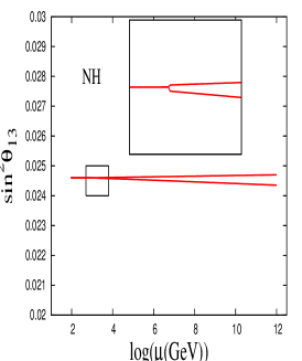
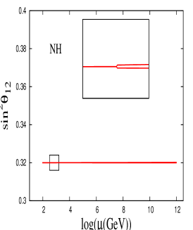
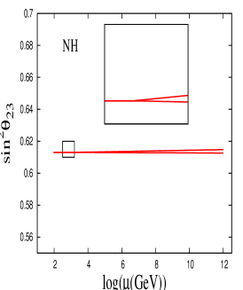
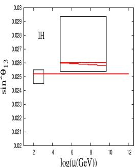
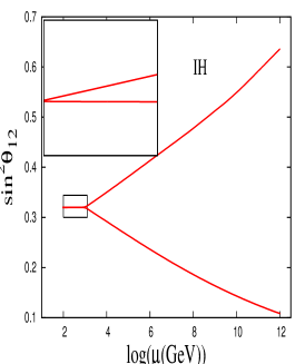
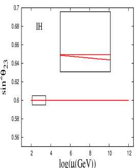
Figs (1) and (2) depict the running of the mixing angles for NH and IH respectively. At low scale we start with best fit values for angles given in Table(1) for the respective hierarchies. All phases except leptonic phases are varied randomly. The numerical value for $y_{\nu}$ in this case is taken to be $0.24$. It should be noted that in this model the magnitude of $y_{s}$ is very small, ${\mathcal{O}}(10^{-11})$. Additionally in the running of the neutrino parameters the factor that plays the crucial role is $Y_{\nu}^{\dagger}Y_{\nu}$. In this case the contribution $Y_{S}^{\dagger}Y_{S}$ appears as an additive factor to $Y_{\nu}^{\dagger}Y_{\nu}$. Hence, the contribution is negligible. In hierarchical case it appears angles do not run considerably, except the angle, $\theta_{12}$ for IH case. While going from low to high scale they retain their low scale values. The effect of threshold correction is more prominent in IH case than in NH case as shown in Fig.(1) and Fig.(2). For $\theta_{13}$ since the running is proportional to $m_{3}$ this angle is not not expected to run in this model since it has $m_{3}=0$. However the small amount running as seen in the figure can be interpreted from the ${\mathcal{O}}(\sin\theta^{\Lambda}_{13})$ terms in the analytical expression.

In general it is seen that the running of angles due to RG evolution is unidirectional i.e. either they increase or decrease while going from low to high scale Antusch et al. (2003). But as seen from our results the angles are running in both directions; for example in fig.(2) the angle, $\theta_{12}$ is running in both directions. This feature comes into picture because of interplay between different $\Delta_{i}$’s that appear in Eq.(37). The maximum running comes when the magnitude of $\Delta_{e}$ is dominant as compared to $\Delta_{\mu}$ and $\Delta_{\tau}$ e.g. for a particular choice of phases, $\delta=0$ and $\alpha=0$, $\Delta_{e}\simeq 0.94$, $\Delta_{\mu}\simeq 5.7\times 10^{-4}$ and $\Delta_{\tau}\simeq 5.8\times 10^{-2}$. Whereas the minimum running comes when the combined $\Delta_{\mu}$ and $\Delta_{\tau}$ are dominant in magnitude as compared to $\Delta_{e}$. This happens for another choice of phases, $\delta=0$ and $\alpha=\pi/2$ resulting $\Delta_{e}\simeq 3.1\times 10^{-2}$, $\Delta_{\mu}\simeq 0.42$ and $\Delta_{\tau}\simeq 0.55$. Thus this feature is unique to RG evolution including threshold effect. Also from Eq.(39) it is easy to check that the running of $\theta_{12}$ is proportional to $1/r$ which enhances the effect.

Figure 1: Running of angles for normal hierarchy from low to high scale. At low energy we have taken the best fit values given in Table (1) for normal hierarchy. The Dirac CP phase and Majorana phases are varied randomly. The respective figures show the maxima and mainima of the running of the angles which appear at the threshold point as shown in the insets.

Figure 2: Running of angles for inverted hierarchy. At low energy we have taken the best fit values given in Table (1) for inverted hierarchy. the Dirac CP phase and Majorana phases are varied randomly. The respective figures show the maxima and minima of the running of the angles which appear at the threshold point as shown in the insets.

Figure 3: Running masses, $m_{2}(\mu)$ and $m_{3}(\mu)$ for normal hierarchy from low scale to high scale. For this case we have taken $m_{1}=0$ and the other two masses are reconstructed from experimental values at low energy.

Figure 4: Running of masses $m_{1}(\mu)$ and $m_{2}(\mu)$ for inverted hierarchy from low scale to high scale.For this case we have taken $m_{3}=0$ and the other two masses are reconstructed from experimental values at low energy.

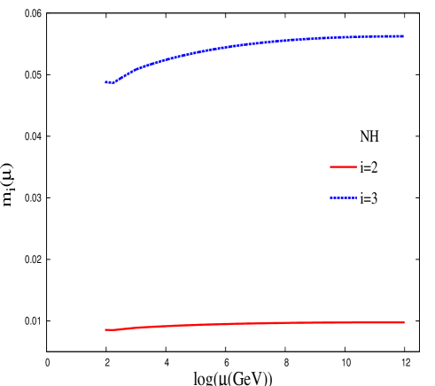
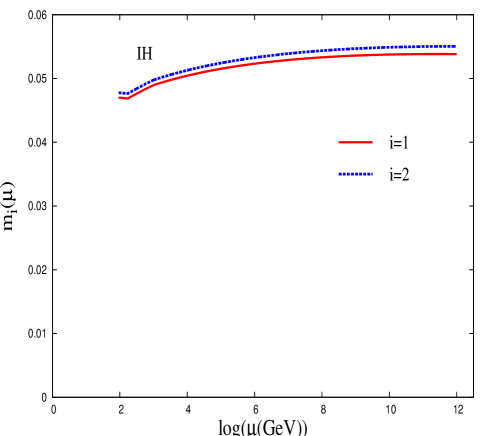
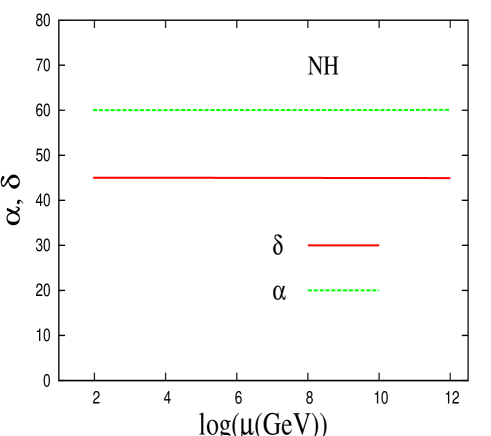
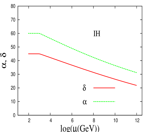
The Figs.(3) and (4) show the running of the masses. It appears that the masses do not run much. Form the analytical expressions for masses given in Eq.(34), one can see the running of masses is proportional to the respective masses themselves at leading order. For NH the masses, $m_{1}$ and $m_{2}$ are plotted with renormalization scale as $m_{3}=0$ in this case. Since for IH case $m_{3}=0$, the masses $m_{1}$ and $m_{2}$ are plotted. In Figs. 5 and 6 we show the running of the phases. In this case since one of the mass eigenvalues is zero there is only one independent Majorana phase. The figures demonstrate that for NH the phases do not run. This feature can be understood from the analytical expressions given in Eq.(31). One can see the running of the Majorana phases is proportional to $m_{1}$ which is vanishing for normal hierarchy in this model. However for IH there is considerable running of the phases. For inverted hierarchy the phases run considerably because of the enhancement coming from the solar mass squared difference that appears in the denominator of $a_{i}$’s in Eq.(31).

Figure 5: Running phases for normal hierarchy from low scale to high scale. Since in this case one of the masses, $m_{1}=0$ there is one independent Majorana phase.

Figure 6: Running phases for inverted hierarchy from low scale to high scale. In this case one of the masses, $m_{3}=0$ and hence there is one independent Majorana phase.

V.2 Quasidegenrate Neutrinos

In this section we consider adding three heavy right handed neutrinos, $N_{R}$ degenerate in mass to the SM. The Lagrangian is given in Eq.(1).Here $Y_{\nu}$ is a $3\times 3$ matrix.Using the parametrization in Casas and Ibarra (2001) $Y_{\nu}$ can be reconstructed from Eq. (3) as

$$Y_{\nu}=\frac{2}{v^{2}}\sqrt{M^{d}_{R}}R\sqrt{m^{d}_{\nu}}U^{\dagger}{}$$ (56)

where $M^{d}_{R}$ and $m^{d}_{\nu}$ are the diagonalized mass matrix for heavy and light neutrinos respectively. $U$ is the standard $U_{\rm PMNS}$ matrix diagonalizing the mass matrix $Um_{\nu}U^{\dagger}=m^{d}_{\nu}$. $R$ is a complex orthogonal matrix, $RR^{T}=I$. The $R$ matrix can be parametrized as

$$R=Oe^{iA}$$ (57)

where $O$ and $A$ are real matrices. The condition of orthogonality implies that $O$ is orthogonal and $A$ is antisymmetric.

$$\begin{pmatrix}0&a&b\\ -a&0&c\\ -b&-c&0\end{pmatrix}$$ (58)

with real $a,b,c$. In particular

$$e^{iA}=I-\frac{\cosh\omega-1}{\omega^{2}}A^{2}+i\frac{\sinh\omega}{\omega}A$$ (59)

where $\omega=\sqrt{a^{2}+b^{2}+c^{2}}$. Using Eq.(58) and Eq.(59) in Eq.(56) we can get $Y_{\nu}$ for our numerical work. It can be observed that the parameter $\omega$ plays an important role in determining the magnitude of $Y_{\nu}$. For our numerical work we have taken $\omega=11.6$ and $a=b=c$. Similar kind of assumption can be found in Rodejohann and Zhang (2012); Pascoli et al. (2003). For this particular choice of $\omega$ and with $M_{R}$ at $1$ TeV, the order of ${\rm Tr}(Y^{\dagger}_{\nu}Y_{\nu})\simeq 0.06$.

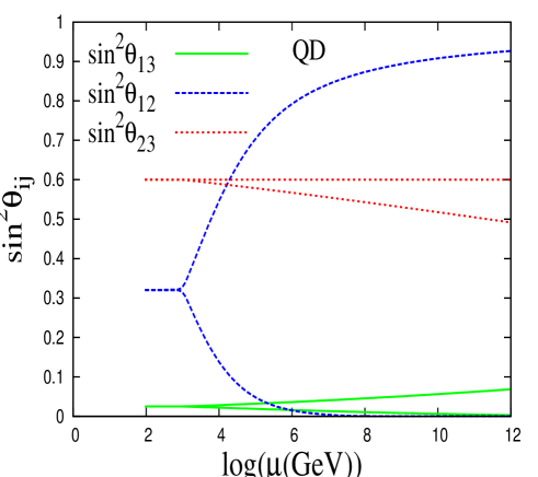
The Fig. (7) shows the running of the mixing angles for QD neutrinos. The angles seem to run considerably covering a wide range of values at high scale. In particular at high scale $\sin^{2}\theta_{12}$ can accommodate the range from zero to $\simeq 0.92$. Both the angles; $\theta_{12}$ and $\theta_{13}$ exhibit bidirectional running whereas the running of $\theta_{23}$ is unidirectional. This behavior of running of angles can be understood from the analytical expressions given in Eqs.(37) and (40) and with specific numerical values of $\Delta_{e}\,,\Delta_{\mu}\,\text{and}\,\Delta_{\tau}$. For example we find for a particular choice of phase, the magnitude of $\Delta_{e}\simeq 3.08\times 10^{-2}$, $\Delta_{\mu}\simeq 1.9\times 10^{-2}$ and $\Delta_{\tau}\simeq 6.13\times 10^{-3}$. For some other choice of phases, the magnitude of $\Delta_{e}\simeq 3.3\times 10^{-3}$, $\Delta_{\mu}\simeq 5.5\times 10^{-2}$ and $\Delta_{\tau}\simeq 4.8\times 10^{-3}$. Also in our numerical study, $\Delta_{\mu}$ is always greater than that of $\Delta_{\tau}$ whereas the magnitude of $\Delta_{e}$ can be more or less than that of $\Delta_{\mu}$. For the case of angle $\theta_{13}$, though $\Delta_{\mu}$ is always greater than $\Delta_{\tau}$ the relative sign difference between $\cos\alpha_{1}$ and $\cos\alpha_{2}$ appearing in the expression of $K_{\mu 13}$ results in bidirectional running of the same. So even if at high scale the angle $\theta_{13}$ can be of zero value the threshold effect can result in nonzero value at low scale.

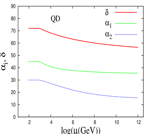
In general the running for the QD case is more than that of hierarchical case, in presence of threshold effects. This is highly dependent on the magnitude and form of $Y_{\nu}$. And using Casas-Ibarra parametrization the magnitude of $Y_{\nu}$ can be magnified even for a low seesaw scale. Fig.(8) shows the running of the phases. One can see the effect of threshold correction on the running of phases at $1$ TeV. This also depends on the form and magnitude of $Y_{\nu}$ chosen.

Figure 7: Running of angles for quasidegenerate neutrinos. At low energy we have taken the common mass $m_{0}=0.2$eV. The Dirac CP phase and Majorana phases are varied randomly. The respective figures show the maxima and minima of the running of the angles which appear at the threshold point.

Figure 8: Running of phases for quasidegenerate neutrinos from low scale to high scale.

VI Conclusion

We consider the threshold effect in renormalization group (RG) evolution of the neutrino masses and mixing arising in TeV scale seesaw models. In such models the heavy states stay coupled to the theory once their mass threshold is crossed and can give rise to additional terms in the beta functions. We obtain the analytical expressions for the coefficients governing the running of masses, mixing angles and phases using the factorization technique including these additional terms. The threshold corrections can give rise to an enhanced running effect with the coefficient $\Delta_{\tau}\simeq 10^{-3}$ as compared to $\Delta_{\tau}\simeq 10^{-5}$ where corrections due to threshold effect are absent. The actual running depends on the form of the Yukawa coupling matrix $Y_{\nu}$. We perform a numerical analysis of this in the bottom up approach using two specific models where the matrix $Y_{\nu}$ can be reconstructed easily. The first case considered by us is the minimal linear seesaw model with hierarchical light neutrinos having one of the mass eigenvalues as zero. The heavy neutrinos are pseudo-Dirac in nature and both have mass $\sim$ TeV. Thus the model contains a single threshold at the TeV scale. In this case for NH we do not obtain appreciable running for the mixing angles, masses and phases. For IH, the mixing angle $\theta_{12}$ and the phases show considerable running effect. The unique feature of threshold effect is that the mixing angle $\theta_{12}$ can increase or decrease from low to high scale depending on initial choice of phases i.e the running is not unidirectional. The second example that we consider is a model with quasidegenerate light neutrinos. For this case we reconstruct the Yukawa matrix in terms of the low scale parameters using the Casas-Ibarra parametrization where the three heavy neutrinos are taken to be degenerate in mass. For this case we obtain considerable running effect for the mixing angle and the phases. In this case two out of the three mixing angles ($\theta_{12}\,,\theta_{13}$) run in both directions. Also the running effect is more than that of minimal linear seesaw model. To conclude, in presence of threshold effects the running of the neutrino parameters depend on the form of the Yukawa matrix apart from the mass spectrum and the phases.

Acknowledgment

The authors would like to thank Amol Dighe for useful discussions.

Appendix A Analytical results for Majorana and leptonic phases

In this section we give the analytic expressions of the coefficients that appear in the perturbation of Dirac, Majorana and leptonic phases (the analytic expressions of the coefficients of the mixing angles for non zero $\theta_{13}$ can be found in Bergstrom et al. (2010)).

$$\delta^{\lambda} = \delta^{\Lambda}+d_{e}\Delta_{e}+d_{\mu}\Delta_{\mu}+d_{\tau}\Delta_{\tau}$$

$$\alpha^{\lambda}_{i} = \alpha^{\Lambda}_{i}+a_{e_{i}}\Delta_{e}+a_{\mu_{i}}\Delta_{\mu}+a_{\tau_{i}}\Delta_{\tau}$$ (60)

$$\Phi_{i}^{\lambda}=\Phi_{i}^{\Lambda}+p_{e_{i}}\Delta_{e}+p_{\mu_{i}}\Delta_{\mu}+p_{\tau_{i}}\Delta_{\tau}$$ (61)

We define a quantity $\xi$ such that

$$\xi_{ij}=\frac{m_{i}-m_{j}}{m_{i}+m_{j}}$$ (62)

The expressions are given by

$$d_{e} = -\,\frac{1}{2}\left(\frac{1}{\xi_{12}}-\xi_{12}\right)\sin\left(\alpha_{1}^{\Lambda}-\alpha_{2}^{\Lambda}\right)+\frac{1}{2}\left[\left(\frac{1}{\xi_{13}}-\xi_{13}\right)\cos^{2}\theta_{12}^{\Lambda}\sin\left(\alpha_{1}^{\Lambda}-2\delta^{\Lambda}\right)\right.$$

$$-\,\left(\frac{1}{\xi_{32}}-\xi_{32}\right)\sin^{2}\theta_{12}^{\Lambda}\sin\left(\alpha_{2}^{\Lambda}-2\,\delta^{\Lambda}\right)\bigg{]}$$

$$+\,2\cot 2\,\theta_{23}^{\Lambda}\left[\frac{1}{4}\left(\frac{1}{\xi_{13}}-\xi_{13}\right)\sin\left(\alpha_{1}^{\Lambda}-\delta^{\Lambda}\right)+\frac{1}{4}\left(\frac{1}{\xi_{32}}-\xi_{32}\right)\sin\left(\alpha_{2}^{\Lambda}-\delta^{\Lambda}\right)\right.$$

$$\left.+\,\frac{1}{4}\left(\frac{m_{3}^{\Lambda}}{m_{2}^{\Lambda}}\left(\frac{1}{\xi_{32}}-\xi_{32}\right)+\frac{m_{3}^{\Lambda}}{m_{1}^{\Lambda}}\left(\frac{1}{\xi_{13}}-\xi_{13}\right)\right)\sin\delta^{\Lambda}\right]\sin 2\theta_{12}^{\Lambda}\sin\theta_{13}^{\Lambda}$$

$$-\,\text{cosec}\,\delta^{\Lambda}\text{cosec}\,\theta_{12}^{\Lambda}\,\text{cosec}\,\theta_{23}^{\Lambda}\,\sec\theta_{12}^{\Lambda}\,\sec\theta_{23}^{\Lambda}\left[\frac{1}{2}\left\{-\frac{1}{2}\left(\frac{1}{\xi_{13}}-\xi_{13}\right)\times\right.\right.$$

$$\left.\left.\cos\left(\alpha_{1}^{\Lambda}-\delta^{\Lambda}\right)+\left(-\frac{1}{2}\left(\frac{1}{\xi_{32}}-\xi_{32}\right)\cos\left(\alpha_{2}^{\Lambda}-\delta^{\Lambda}\right)+\frac{1}{4}\left(\frac{1}{\xi_{12}}-\xi_{12}\right)\right.\right.\right.$$

$$\left.\left.\left(\left(\frac{m_{1}^{\Lambda}}{m_{2}^{\Lambda}}+\frac{m_{2}^{\Lambda}}{m_{1}^{\Lambda}}\right)\cos\delta^{\Lambda}+2\cos\left(\alpha_{1}^{\Lambda}-\alpha_{2}^{\Lambda}+\delta^{\Lambda}\right)\right)\right)\right\}\cos\theta_{12}^{\Lambda}\sin^{3}\theta_{12}^{\Lambda}$$

$$+\,2\cos\delta^{\Lambda}\left\{\left(-1-\frac{1}{4}\frac{m_{1}^{\Lambda}}{m_{3}^{\Lambda}}\left(\frac{1}{\xi_{13}}-\xi_{13}\right)-\frac{3}{4}\frac{m_{2}^{\Lambda}}{m_{3}^{\Lambda}}\left(\frac{1}{\xi_{32}}-\xi_{32}\right)\right)\right.$$

$$+\,\left(\frac{1}{2}\left(\left(\frac{m_{1}^{\Lambda}}{m_{2}^{\Lambda}}+\frac{m_{2}^{\Lambda}}{m_{1}^{\Lambda}}\right)\left(\frac{1}{\xi_{12}}-\xi_{12}\right)-\frac{1}{2}\frac{m_{2}^{\Lambda}}{m_{3}^{\Lambda}}\left(\frac{1}{\xi_{32}}-\xi_{32}\right)-\frac{1}{2}\frac{m_{1}^{\Lambda}}{m_{3}^{\Lambda}}\left(\frac{1}{\xi_{13}}-\xi_{13}\right)\right)\right.$$

$$\left.+\,\left(\frac{1}{\xi_{12}}-\xi_{12}\right)\cos\left(\alpha_{1}^{\Lambda}-\alpha_{2}^{\Lambda}\right)\right)\cos 2\theta_{12}^{\Lambda}-\frac{1}{4}\left(\frac{1}{\xi_{13}}-\xi_{13}\right)\cos\left(\alpha_{1}^{\Lambda}-2\delta^{\Lambda}\right)\times$$

$$\left.\left(-1+3\cos 2\theta_{12}^{\Lambda}\right)-\frac{1}{4}\left(\frac{1}{\xi_{32}}-\xi_{32}\right)\cos\left(\alpha_{2}^{\Lambda}-2\delta^{\Lambda}\right)\left(1+3\cos 2\theta_{12}^{\Lambda}\right)\right\}\times$$

$$\sin 2\theta_{12}^{\Lambda}\bigg{]}\sin^{2}\theta_{13}^{\Lambda}\sin 2\theta_{23}^{\Lambda}$$ (63)

$$d_{\mu} = \frac{1}{8}\left[\left(\frac{1}{\xi_{13}}-\xi_{13}\right)\left(\frac{m_{3}^{\Lambda}}{m_{1}^{\Lambda}}\sin\delta^{\Lambda}-\sin\left(\alpha_{1}^{\Lambda}-\delta^{\Lambda}\right)\right)+\left(\frac{1}{\xi_{32}}-\xi_{32}\right)\left(\frac{m_{3}^{\Lambda}}{m_{2}^{\Lambda}}\,\sin\delta^{\Lambda}\right.\right.$$

$$-\,\sin\left(\alpha_{2}^{\Lambda}-\delta^{\Lambda}\right)\bigg{)}\bigg{]}\frac{\sin 2\theta_{12}^{\Lambda}\sin 2\theta_{23}^{\Lambda}}{\sin\theta_{13}^{\Lambda}}$$

$$+ \frac{1}{2}\left[\left(\frac{1}{\xi_{12}}-\xi_{12}\right)\cos^{2}\theta_{23}^{\Lambda}\sin\left(\alpha_{1}^{\Lambda}-\alpha_{2}^{\Lambda}\right)+\left(\frac{1}{\xi_{32}}-\xi_{32}\right)\Big{(}\cos^{2}\theta_{12}^{\Lambda}\cos 2\theta_{23}^{\Lambda}\sin\alpha_{2}^{\Lambda}\right.$$

$$+\,\sin^{2}\theta_{12}^{\Lambda}\sin^{2}\theta_{23}^{\Lambda}\sin\left(\alpha_{2}^{\Lambda}-2\delta^{\Lambda}\right)\Big{)}-\left(\frac{1}{\xi_{13}}-\xi_{13}\right)\Big{(}\sin^{2}\theta_{12}^{\Lambda}\cos 2\theta_{23}^{\Lambda}\sin\alpha_{1}^{\Lambda}$$

$$+\,\cos^{2}\theta_{12}^{\Lambda}\sin^{2}\theta_{23}^{\Lambda}\sin\left(\alpha_{1}^{\Lambda}-2\delta^{\Lambda}\right)\Big{)}\bigg{]}$$

$$+ \left[\text{cosec}2\theta_{12}^{\Lambda}\left\{\cos^{2}\theta_{12}^{\Lambda}\left(\frac{1}{2}\left(\frac{1}{\xi_{12}}-\xi_{12}\right)\sin\left(\alpha_{1}^{\Lambda}-\alpha_{2}^{\Lambda}-\delta^{\Lambda}\right)+\frac{1}{4}\left(\frac{1}{\xi_{32}}-\xi_{32}\right)\times\right.\right.\right.$$

$$\left(-1+3\cos 2\theta_{12}^{\Lambda}\right)\sin\left(\alpha_{2}^{\Lambda}-\delta^{\Lambda}\right)\bigg{)}+\left(\frac{1}{16}\left(4\left(\frac{m_{1}^{\Lambda}}{m_{2}^{\Lambda}}+\frac{m_{2}^{\Lambda}}{m_{1}^{\Lambda}}\right)\left(\xi_{12}-\frac{1}{\xi_{12}}\right)\right.\right.$$

$$\left.-\,5\,\frac{m_{2}^{\Lambda}}{m_{3}^{\Lambda}}\left(\frac{1}{\xi_{32}}-\xi_{32}\right)-5\,\frac{m_{1}^{\Lambda}}{m_{3}^{\Lambda}}\left(\frac{1}{\xi_{13}}-\xi_{13}\right)\right)+\left(\frac{1}{4}\left(\frac{m_{1}^{\Lambda}}{m_{3}^{\Lambda}}\left(\frac{1}{\xi_{13}}-\xi_{13}\right)\right.\right.$$

$$\left.-\,\frac{m_{3}^{\Lambda}}{m_{2}^{\Lambda}}\left(\frac{1}{\xi_{32}}-\xi_{32}\right)\right)\cos 2\theta_{12}^{\Lambda}+\frac{1}{16}\left(\frac{m_{3}^{\Lambda}}{m_{2}^{\Lambda}}\left(\frac{1}{\xi_{32}}-\xi_{32}\right)+\frac{m_{3}^{\Lambda}}{m_{1}^{\Lambda}}\left(\frac{1}{\xi_{13}}-\xi_{13}\right)\right)\times$$

$$\cos 4\theta_{12}^{\Lambda}\bigg{)}\bigg{)}\sin\,\delta^{\Lambda}-\left(\frac{1}{4}\left(\frac{1}{\xi_{13}}-\xi_{13}\right)\left(1+3\cos 2\theta_{12}^{\Lambda}\right)\sin\left(\alpha_{1}^{\Lambda}-\delta^{\Lambda}\right)\right.$$

$$\left.+\,\frac{1}{2}\left(\frac{1}{\xi_{12}}-\xi_{12}\right)\sin\left(\alpha_{1}^{\Lambda}-\alpha_{2}^{\Lambda}+\delta^{\Lambda}\right)\right)\sin^{2}\theta_{12}^{\Lambda}\bigg{\}}\sin 2\theta_{23}^{\Lambda}+\left\{\frac{1}{4}\left(\frac{1}{\xi_{13}}-\xi_{13}\right)\times\right.$$

$$\sin\left(\alpha_{1}^{\Lambda}-\delta^{\Lambda}\right)+\frac{1}{4}\left(\frac{1}{\xi_{32}}-\xi_{32}\right)\sin\left(\alpha_{2}^{\Lambda}-\delta^{\Lambda}\right)+\frac{1}{4}\left(\frac{m_{3}^{\Lambda}}{m_{2}^{\Lambda}}\left(\frac{1}{\xi_{32}}-\xi_{32}\right)\right.$$

$$\left.\left.+\,\frac{m_{3}^{\Lambda}}{m_{1}^{\Lambda}}\left(\frac{1}{\xi_{13}}-\xi_{13}\right)\right)\sin\delta^{\Lambda}\right\}\sin 2\theta_{12}^{\Lambda}\tan\theta_{23}^{\Lambda}\bigg{]}\sin\theta_{13}^{\Lambda}$$

$$+ \left[-\frac{3}{16}\left(\frac{1}{\xi_{13}}-\xi_{13}\right)\cos\left(\alpha_{1}^{\Lambda}-\delta^{\Lambda}\right)-\frac{5}{16}\left(\frac{1}{\xi_{32}}-\xi_{32}\right)\cos\left(\alpha_{2}^{\Lambda}-\delta^{\Lambda}\right)\right.$$

$$+\,\frac{1}{8}\left\{-\frac{m_{1}^{\Lambda}}{m_{3}^{\Lambda}}\left(\frac{1}{\xi_{13}}-\xi_{13}\right)+2\frac{m_{2}^{\Lambda}}{m_{1}^{\Lambda}}\left(\frac{1}{\xi_{12}}-\xi_{12}\right)-3\frac{m_{2}^{\Lambda}}{m_{3}^{\Lambda}}\left(\frac{1}{\xi_{32}}-\xi_{32}\right)\right\}\cos\,\delta^{\Lambda}$$

$$+\,\frac{1}{4}\left(\frac{1}{\xi_{32}}-\xi_{32}\right)\cos\left(\alpha_{1}^{\Lambda}-\alpha_{2}^{\Lambda}+\delta^{\Lambda}\right)-\frac{1}{16}\left(\frac{1}{\xi_{13}}-\xi_{13}\right)\cos\left(\alpha_{1}^{\Lambda}-3\delta^{\Lambda}\right)\times$$

$$\left(-1+3\cos 2\theta_{12}^{\Lambda}\right)-\frac{1}{16}\left(\frac{1}{\xi_{32}}-\xi_{32}\right)\cos\left(\alpha_{2}^{\Lambda}-3\delta^{\Lambda}\right)\left(1+3\cos 2\theta_{12}^{\Lambda}\right)$$

$$+\,\cos 2\theta_{12}^{\Lambda}\left\{\left(\frac{1}{16}\left(\frac{1}{\xi_{13}}-\xi_{13}\right)+\frac{1}{4}\left(\frac{1}{\xi_{32}}-\xi_{32}\right)\cos\alpha_{2}^{\Lambda}\right)\cos\left(\alpha_{1}^{\Lambda}-\delta^{\Lambda}\right)\right.$$

$$+\frac{1}{16}\left(\frac{1}{\xi_{32}}-\xi_{32}\right)\cos\left(\alpha_{2}^{\Lambda}-\delta^{\Lambda}\right)+\frac{1}{8}\left(\left(\frac{m_{1}^{\Lambda}}{m_{2}^{\Lambda}}+\frac{m_{2}^{\Lambda}}{m_{1}^{\Lambda}}\right)\left(\frac{1}{\xi_{12}}-\xi_{12}\right)\right.$$

$$\left.-\frac{m_{2}^{\Lambda}}{m_{3}^{\Lambda}}\left(\frac{1}{\xi_{32}}-\xi_{32}\right)-\frac{m_{1}^{\Lambda}}{m_{3}^{\Lambda}}\left(\frac{1}{\xi_{13}}-\xi_{13}\right)\right)\cos\delta^{\Lambda}$$

$$\left.\left.+\,\frac{1}{4}\left(\frac{1}{\xi_{32}}-\xi_{32}\right)\sin\alpha_{2}^{\Lambda}\sin\left(\alpha_{1}^{\Lambda}-\delta^{\Lambda}\right)\right\}\right]\text{cosec}\,\delta^{\Lambda}\sin^{2}\theta_{23}^{\Lambda}\sin^{2}\theta_{13}^{\Lambda}$$ (64)

$$d_{\tau} = \frac{1}{8}\left[\left(\frac{1}{\xi_{13}}-\xi_{13}\right)\sin\left(\alpha_{1}^{\Lambda}-\delta^{\Lambda}\right)+\left(\frac{1}{\xi_{32}}-\xi_{32}\right)\sin\left(\alpha_{2}^{\Lambda}-\delta^{\Lambda}\right)-\left\{\frac{m_{3}^{\Lambda}}{m_{2}^{\Lambda}}\left(\frac{1}{\xi_{32}}-\xi_{32}\right)\right.\right.$$

$$\left.\left.+\,\frac{m_{3}^{\Lambda}}{m_{1}^{\Lambda}}\left(\frac{1}{\xi_{13}}-\xi_{13}\right)\right\}\sin\,\delta^{\Lambda}\right]\frac{\sin 2\theta_{12}^{\Lambda}\sin 2\theta_{23}^{\Lambda}}{\sin\theta_{13}^{\Lambda}}$$

$$+ \frac{1}{2}\left[\left\{\cos^{2}\theta_{12}^{\Lambda}\left(-\left(\frac{1}{\xi_{32}}-\xi_{32}\right)\cos 2\theta_{23}^{\Lambda}\sin\alpha_{2}^{\Lambda}-\left(\frac{1}{\xi_{13}}-\xi_{13}\right)\cos^{2}\theta_{23}^{\Lambda}\times\right.\right.\right.$$

$$\sin\left(\alpha_{1}^{\Lambda}-2\,\delta^{\Lambda}\right)\bigg{)}+\left(\left(\frac{1}{\xi_{13}}-\xi_{13}\right)\cos 2\theta_{23}^{\Lambda}\sin\alpha_{1}^{\Lambda}+\left(\frac{1}{\xi_{32}}-\xi_{32}\right)\cos^{2}\theta_{23}^{\Lambda}\times\right.$$

$$\left.\sin\left(\alpha_{2}^{\Lambda}-2\,\delta^{\Lambda}\right)\bigg{)}\sin^{2}\theta_{12}^{\Lambda}\bigg{\}}+\left(\frac{1}{\xi_{12}}-\xi_{12}\right)\sin\left(\alpha_{1}^{\Lambda}-\alpha_{2}^{\Lambda}\right)\sin^{2}\theta_{23}^{\Lambda}\right]$$

$$+ \left[\frac{1}{4}\left(\frac{1}{\xi_{12}}-\xi_{12}\right)\cos\left(\alpha_{1}^{\Lambda}-\delta^{\Lambda}\right)\sin\alpha_{2}^{\Lambda}-\frac{1}{8}\left(\frac{1}{\xi_{12}}-\xi_{12}\right)\left(1+2\cos 2\theta_{12}^{\Lambda}\right)\times\right.$$

$$\sin\left(\alpha_{1}^{\Lambda}-\alpha_{2}^{\Lambda}-\delta^{\Lambda}\right)-\frac{3}{16}\left(\frac{1}{\xi_{32}}-\xi_{32}\right)\sin\left(\alpha_{2}^{\Lambda}-\delta^{\Lambda}\right)-\frac{1}{4}\left(\frac{1}{\xi_{32}}-\xi_{32}\right)\times$$

$$\sin\left(\alpha_{2}^{\Lambda}-\delta^{\Lambda}\right)\cos 2\theta_{12}^{\Lambda}-\frac{1}{16}\left(\frac{1}{\xi_{32}}-\xi_{32}\right)\sin\left(\alpha_{2}^{\Lambda}-\delta^{\Lambda}\right)\cos 4\theta_{12}^{\Lambda}-\frac{1}{8}\left(\frac{1}{\xi_{12}}-\xi_{12}\right)\times$$

$$\sin\left(\alpha_{1}^{\Lambda}+\alpha_{2}^{\Lambda}-\delta^{\Lambda}\right)+\frac{1}{8}\left\{-2\left(\frac{m_{1}^{\Lambda}}{m_{2}^{\Lambda}}+\frac{m_{2}^{\Lambda}}{m_{1}^{\Lambda}}\right)\left(\frac{1}{\xi_{12}}-\xi_{12}\right)+\frac{3}{2}\frac{m_{1}^{\Lambda}}{m_{3}^{\Lambda}}\left(\frac{1}{\xi_{13}}-\xi_{13}\right)\right.$$

$$\left.+\,\frac{3}{2}\frac{m_{2}^{\Lambda}}{m_{3}^{\Lambda}}\left(\frac{1}{\xi_{32}}-\xi_{32}\right)\right\}\sin\,\delta^{\Lambda}+\frac{1}{4}\left\{-\frac{1}{4}\frac{m_{1}^{\Lambda}}{m_{3}^{\Lambda}}\left(\frac{1}{\xi_{13}}-\xi_{13}\right)+\frac{1}{4}\frac{m_{3}^{\Lambda}}{m_{2}^{\Lambda}}\left(\frac{1}{\xi_{32}}-\xi_{32}\right)\right\}\times$$

$$\cos 2\theta_{12}^{\lambda}\sin\,\delta^{\Lambda}+\frac{1}{16}\left\{\frac{m_{3}^{\Lambda}}{m_{2}^{\Lambda}}\left(\frac{1}{\xi_{32}}-\xi_{32}\right)+\frac{1}{4}\frac{m_{3}^{\Lambda}}{m_{1}^{\Lambda}}\left(\frac{1}{\xi_{13}}-\xi_{13}\right)\right\}\cos 4\theta_{12}^{\Lambda}\sin\,\delta^{\Lambda}$$

$$+\frac{1}{2}\left(\frac{1}{\xi_{12}}-\xi_{12}\right)\sin\left(\alpha_{1}^{\Lambda}-\alpha_{2}^{\Lambda}+\delta^{\Lambda}\right)\sin^{2}\theta_{12}^{\Lambda}-\frac{1}{2}\left(\frac{1}{\xi_{13}}-\xi_{13}\right)\sin\left(\alpha_{1}^{\Lambda}-\delta^{\Lambda}\right)\times$$

$$\sin^{4}\theta_{12}^{\Lambda}+\cos 2\theta_{23}^{\Lambda}\left\{\cos^{2}\theta_{23}^{\Lambda}\left(\frac{1}{2}\left(\frac{1}{\xi_{12}}-\xi_{12}\right)\sin\left(\alpha_{1}^{\Lambda}-\alpha_{2}^{\Lambda}+\delta^{\Lambda}\right)+\frac{1}{4}\left(\frac{1}{\xi_{32}}-\xi_{32}\right)\times\right.\right.$$

$$\left(-1+3\cos 2\theta_{12}^{\Lambda}\right)\sin\left(\alpha_{2}^{\Lambda}-\delta^{\Lambda}\right)\bigg{)}+\left(\frac{1}{8}\left(2\left(\frac{m_{1}^{\Lambda}}{m_{2}^{\Lambda}}+\frac{m_{2}^{\Lambda}}{m_{1}^{\Lambda}}\right)\left(\frac{1}{\xi_{12}}-\xi_{12}\right)-\frac{5}{2}\frac{m_{2}^{\Lambda}}{m_{3}^{\Lambda}}\times\right.\right.$$

$$\left.\left(\frac{1}{\xi_{32}}-\xi_{32}\right)-\frac{5}{2}\frac{m_{1}^{\Lambda}}{m_{3}^{\Lambda}}\left(\frac{1}{\xi_{13}}-\xi_{13}\right)\right)+\left(\left(\frac{1}{4}\frac{m_{1}^{\Lambda}}{m_{3}^{\Lambda}}\left(\frac{1}{\xi_{13}}-\xi_{13}\right)-\frac{1}{4}\frac{m_{3}^{\Lambda}}{m_{2}^{\Lambda}}\left(\frac{1}{\xi_{32}}-\xi_{32}\right)\right)\times\right.$$ (65)

$$\left.\left.\cos 2\theta_{12}^{\Lambda}+\frac{1}{16}\left(\frac{m_{3}^{\Lambda}}{m_{2}^{\Lambda}}\left(\frac{1}{\xi_{32}}-\xi_{32}\right)+\frac{m_{3}^{\Lambda}}{m_{1}^{\Lambda}}\left(\frac{1}{\xi_{13}}-\xi_{13}\right)\right)\cos 4\theta_{12}^{\Lambda}\right)\right)\sin\,\delta^{\Lambda}$$

$$-\,\left(\frac{1}{4}\left(\frac{1}{\xi_{13}}-\xi_{13}\right)\left(1+3\cos 2\theta_{12}^{\lambda}\right)\sin\left(\alpha_{1}^{\Lambda}-\delta^{\Lambda}\right)+\frac{1}{2}\left(\frac{1}{\xi_{12}}-\xi_{12}\right)\times\right.$$

$$\left.\left.\sin\left(\alpha_{1}^{\Lambda}-\alpha_{2}^{\Lambda}+\delta^{\Lambda}\right)\bigg{)}\sin^{2}\theta_{12}^{\Lambda}\right\}\right]\text{cot}\theta_{23}^{\Lambda}\text{cosec}2\theta_{12}^{\Lambda}\sin\theta_{13}^{\Lambda}$$

$$+ \left[-\frac{3}{16}\left(\frac{1}{\xi_{13}}-\xi_{13}\right)\cos\left(\alpha_{1}^{\Lambda}-\delta^{\Lambda}\right)-\frac{5}{16}\left(\frac{1}{\xi_{32}}-\xi_{32}\right)\cos\left(\alpha_{2}^{\Lambda}-\delta^{\Lambda}\right)+\frac{1}{8}\left\{-\frac{m_{1}^{\Lambda}}{m_{3}^{\Lambda}}\times\right.\right.$$

$$\left.\left(\frac{1}{\xi_{13}}-\xi_{13}\right)+\left(2\,\frac{m_{2}^{\Lambda}}{m_{1}^{\Lambda}}\left(\frac{1}{\xi_{12}}-\xi_{12}\right)-3\,\frac{m_{2}^{\Lambda}}{m_{3}^{\Lambda}}\left(\frac{1}{\xi_{32}}-\xi_{32}\right)\right)\right\}\cos\,\delta^{\Lambda}$$

$$+\,\frac{1}{4}\left(\frac{1}{\xi_{12}}-\xi_{12}\right)\cos\left(\alpha_{1}^{\Lambda}-\alpha_{2}^{\Lambda}+\delta^{\Lambda}\right)-\frac{1}{16}\left(\frac{1}{\xi_{13}}-\xi_{13}\right)\cos\left(\alpha_{1}^{\Lambda}-3\,\delta^{\Lambda}\right)\times$$

$$\left(-1+3\cos 2\theta_{12}^{\Lambda}\right)-\frac{1}{16}\left(\frac{1}{\xi_{32}}-\xi_{32}\right)\cos\left(\alpha_{2}^{\Lambda}-3\,\delta^{\Lambda}\right)\left(1+3\cos 2\theta_{12}^{\Lambda}\right)+\cos 2\theta_{12}^{\Lambda}\times$$

$$\left\{\left(\frac{1}{16}\left(\frac{1}{\xi_{13}}-\xi_{13}\right)+\frac{1}{4}\left(\frac{1}{\xi_{12}}-\xi_{12}\right)\cos\alpha_{2}^{\Lambda}\right)\cos\left(\alpha_{1}^{\Lambda}-\delta^{\Lambda}\right)+\frac{1}{16}\left(\frac{1}{\xi_{32}}-\xi_{32}\right)\times\right.$$

$$\cos\left(\alpha_{2}^{\Lambda}-\delta^{\Lambda}\right)+\frac{1}{8}\left(\left(\frac{m_{1}^{\Lambda}}{m_{2}^{\Lambda}}+\frac{m_{2}^{\Lambda}}{m_{1}^{\Lambda}}\right)\left(\frac{1}{\xi_{12}}-\xi_{12}\right)-\frac{m_{2}^{\Lambda}}{m_{3}^{\Lambda}}\left(\frac{1}{\xi_{32}}-\xi_{32}\right)-\frac{m_{1}^{\Lambda}}{m_{3}^{\Lambda}}\times\right.$$

$$\left.\left.\left.\left(\frac{1}{\xi_{13}}-\xi_{13}\right)\right)\cos\,\delta^{\Lambda}+\frac{1}{4}\left(\frac{1}{\xi_{12}}-\xi_{12}\right)\sin\alpha_{2}^{\Lambda}\sin\left(\alpha_{1}^{\Lambda}-\delta^{\Lambda}\right)\right\}\right]\times$$

$$\cos^{2}\theta_{23}^{\Lambda}\text{cosec}\,\delta^{\Lambda}\sin^{2}\theta_{13}^{\Lambda}$$

$$p_{e1}=d_{e}+\frac{1}{2}\left[-\left(\frac{1}{\xi_{13}}-\xi_{13}\right)\cos^{2}\theta^{\Lambda}_{12}\sin(\alpha^{\Lambda}_{1}-2\delta^{\Lambda})+\left(\frac{1}{\xi_{32}}-\xi_{32}\right)\sin(\alpha^{\Lambda}_{2}-2\delta^{\Lambda})\sin^{2}\theta^{\Lambda}_{12}\right]$$ (66)

$$a_{e1} = 2p_{e1}+\left(\frac{1}{\xi_{12}}-\xi_{12}\right)\sin(\alpha^{\Lambda}_{1}-\alpha^{\Lambda}_{2})\sin^{2}\theta^{\Lambda}_{12}$$ (67)

$$+ \left[\left(\frac{1}{\xi_{13}}-\xi_{13}\right)\sin(\alpha^{\Lambda}_{2}-2\delta^{\Lambda})-\left(\frac{1}{\xi_{12}}-\xi_{12}\right)\sin(\alpha^{\Lambda}_{1}-\alpha^{\Lambda}_{2})\sin^{2}\theta^{\Lambda}_{12}\right]\sin^{2}\theta^{\Lambda}_{13}$$

$$a_{e2} = 2p_{e1}+\left(\frac{1}{\xi_{12}}-\xi_{12}\right)\cos^{2}\theta^{\Lambda}_{12}\sin(\alpha^{\Lambda}_{1}-\alpha^{\Lambda}_{2})$$ (68)

$$- \left[\left(\frac{1}{\xi_{12}}-\xi_{12}\right)\cos^{2}\theta^{\Lambda}_{12}\sin(\alpha^{\Lambda}_{1}-\alpha^{\Lambda}_{2})+\left(\frac{1}{\xi_{32}}-\xi_{32}\right)\sin(\alpha^{\Lambda}_{2}-2\delta^{\Lambda})\right]\sin^{2}\theta^{\Lambda}_{13}$$

$$p_{\mu 1} = d^{\prime}_{\mu}-\frac{1}{2}\left[-\left(\frac{1}{\xi_{13}}-\xi_{13}\right)\cos^{2}\theta^{\Lambda}_{12}\sin(\alpha^{\Lambda}_{2}-2\delta^{\Lambda})+\left(\frac{1}{\xi_{32}}-\xi_{32}\right)\sin(\alpha^{\Lambda}_{2}-2\delta^{\Lambda})\sin^{2}\theta^{\Lambda}_{12}\right]\sin^{2}\theta^{\Lambda}_{23}$$ (69)

$$+\frac{1}{8}\left[-\left(\frac{1}{\xi_{13}}-\xi_{13}\right)\sin(\alpha^{\Lambda}_{1}-\delta^{\Lambda})-\left(\frac{1}{\xi_{32}}-\xi_{32}\right)\sin(\alpha^{\Lambda}_{2}-\delta^{\Lambda})\right.$$

$$+\left.\left[\frac{m_{3}}{m_{2}}\left(\frac{1}{\xi_{32}}-\xi_{32}\right)+\frac{m_{3}}{m_{1}}\left(\frac{1}{\xi_{13}}-\xi_{13}\right)\right]\sin\delta^{\Lambda}\right]\sin 2\theta^{\Lambda}_{12}\sin 2\theta^{\Lambda}_{23}\sin\theta^{\Lambda}_{13}$$

where $d^{\prime}_{\mu}$ is the terms appearing in $d_{\mu}$ with coefficent of $1/\sin\theta^{\Lambda}_{13}$ term set to zero.

$$a_{\mu 1} = 2p_{\mu 1}-\left(\frac{1}{\xi_{12}}-\xi_{12}\right)\cos^{2}\theta^{\Lambda}_{23}\sin(\alpha^{\Lambda}_{1}-\alpha^{\Lambda}_{2})\sin^{2}\theta^{\Lambda}_{12}$$

$$-\frac{1}{2}\Bigg{[}\cos\delta^{\Lambda}\Big{[}\left(\frac{1}{\xi_{13}}-\xi_{13}\right)\sin\alpha^{\Lambda}_{1}+\left(\frac{1}{\xi_{12}}-\xi_{12}\right)\cos 2\theta^{\Lambda}_{12}\sin(\alpha^{\Lambda}_{1}-\alpha^{\Lambda}_{2})\Big{]}$$

$$+\Big{[}-\frac{m_{1}}{m_{3}}\left(\frac{1}{\xi_{13}}-\xi_{13}\right)+\frac{m_{1}}{m_{2}}\left(\frac{1}{\xi_{12}}-\xi_{12}\right)-\left(\frac{1}{\xi_{13}}-\xi_{13}\right)\cos\alpha^{\Lambda}_{1}-$$

$$\left(\frac{1}{\xi_{12}}-\xi_{12}\right)\cos(\alpha^{\Lambda}_{1}-\alpha^{\Lambda}_{2})\Big{]}\sin\delta^{\Lambda}\Bigg{]}\sin\theta^{\Lambda}_{13}\sin 2\theta^{\Lambda}_{23}\tan\theta^{\Lambda}_{12}$$ (70)

$$+\Big{[}-\left(\frac{1}{\xi_{13}}-\xi_{13}\right)\sin(\alpha^{\Lambda}_{1}-2\delta^{\Lambda})+\left(\frac{1}{\xi_{12}}-\xi_{12}\right)\sin(\alpha^{\Lambda}_{1}-\alpha^{\Lambda}_{2})\sin^{2}\theta^{\Lambda}_{12}\Big{]}\sin^{2}\theta^{\Lambda}_{13}\sin^{2}\theta^{\Lambda}_{23}$$

$$a_{\mu 2} = 2p_{\mu 1}-\left(\frac{1}{\xi_{12}}-\xi_{12}\right)\cos^{2}\theta^{\Lambda}_{23}\sin(\alpha^{\Lambda}_{1}-\alpha^{\Lambda}_{2})\cos^{2}\theta^{\Lambda}_{12}$$

$$-\frac{1}{2}\Bigg{[}\cos\delta^{\Lambda}\Big{[}\left(\frac{1}{\xi_{32}}-\xi_{32}\right)\sin\alpha^{\Lambda}_{2}+\left(\frac{1}{\xi_{12}}-\xi_{12}\right)\cos 2\theta^{\Lambda}_{12}\sin(\alpha^{\Lambda}_{1}-\alpha^{\Lambda}_{2})\Big{]}$$

$$+\Big{[}-\frac{m_{2}}{m_{3}}\left(\frac{1}{\xi_{32}}-\xi_{32}\right)-\frac{m_{2}}{m_{1}}\left(\frac{1}{\xi_{12}}-\xi_{12}\right)+\left(\frac{1}{\xi_{32}}-\xi_{32}\right)\cos\alpha^{\Lambda}_{2}-$$

$$\left(\frac{1}{\xi_{12}}-\xi_{12}\right)\cos(\alpha^{\Lambda}_{1}-\alpha^{\Lambda}_{2})\Big{]}\sin\delta^{\Lambda}\Bigg{]}\sin\theta^{\Lambda}_{13}\sin 2\theta^{\Lambda}_{23}\cot\theta^{\Lambda}_{12}$$

$$+\Big{[}\left(\frac{1}{\xi_{32}}-\xi_{32}\right)\sin(\alpha^{\Lambda}_{2}-2\delta^{\Lambda})+\left(\frac{1}{\xi_{12}}-\xi_{12}\right)\sin(\alpha^{\Lambda}_{1}-\alpha^{\Lambda}_{2})\cos^{2}\theta^{\Lambda}_{12}\Big{]}\sin^{2}\theta^{\Lambda}_{13}\sin^{2}\theta^{\Lambda}_{23}$$

$$p_{\tau 1} = d^{\prime}_{\tau}-\frac{1}{2}\left[-\left(\frac{1}{\xi_{13}}-\xi_{13}\right)\cos^{2}\theta^{\Lambda}_{12}\sin(\alpha^{\Lambda}_{2}-2\delta^{\Lambda})+\left(\frac{1}{\xi_{32}}-\xi_{32}\right)\sin(\alpha^{\Lambda}_{2}-2\delta^{\Lambda})\sin^{2}\theta^{\Lambda}_{12}\right]\cos^{2}\theta^{\Lambda}_{23}$$ (72)

$$-\frac{1}{8}\left[-\left(\frac{1}{\xi_{13}}-\xi_{13}\right)\sin(\alpha^{\Lambda}_{1}-\delta^{\Lambda})-\left(\frac{1}{\xi_{32}}-\xi_{32}\right)\sin(\alpha^{\Lambda}_{2}-\delta^{\Lambda})\right.$$

$$+\left.\left[\frac{m_{3}}{m_{2}}\left(\frac{1}{\xi_{32}}-\xi_{32}\right)+\frac{m_{3}}{m_{1}}\left(\frac{1}{\xi_{13}}-\xi_{13}\right)\right]\sin\delta^{\Lambda}\right]\sin 2\theta^{\Lambda}_{12}\sin 2\theta^{\Lambda}_{23}\sin\theta^{\Lambda}_{13}$$

where $d^{\prime}_{\tau}$ is the terms appearing in $d_{\tau}$ with coefficient of $1/\sin\theta^{\Lambda}_{13}$ term set to zero.

$$a_{\tau 1} = 2p_{\tau 1}-\left(\frac{1}{\xi_{12}}-\xi_{12}\right)\sin^{2}\theta^{\Lambda}_{23}\sin(\alpha^{\Lambda}_{1}-\alpha^{\Lambda}_{2})\sin^{2}\theta^{\Lambda}_{12}$$

$$+\frac{1}{2}\Bigg{[}\cos\delta^{\Lambda}\Big{[}\left(\frac{1}{\xi_{13}}-\xi_{13}\right)\sin\alpha^{\Lambda}_{1}+\left(\frac{1}{\xi_{12}}-\xi_{12}\right)\cos 2\theta^{\Lambda}_{12}\sin(\alpha^{\Lambda}_{1}-\alpha^{\Lambda}_{2})\Big{]}$$

$$+\Big{[}-\frac{m_{1}}{m_{3}}\left(\frac{1}{\xi_{13}}-\xi_{13}\right)+\frac{m_{1}}{m_{2}}\left(\frac{1}{\xi_{12}}-\xi_{12}\right)-\left(\frac{1}{\xi_{13}}-\xi_{13}\right)\cos\alpha^{\Lambda}_{1}-$$

$$\left(\frac{1}{\xi_{12}}-\xi_{12}\right)\cos(\alpha^{\Lambda}_{1}-\alpha^{\Lambda}_{2})\Big{]}\sin\delta^{\Lambda}\Bigg{]}\sin\theta^{\Lambda}_{13}\sin 2\theta^{\Lambda}_{23}\tan\theta^{\Lambda}_{12}$$

$$+\Big{[}-\left(\frac{1}{\xi_{13}}-\xi_{13}\right)\sin(\alpha^{\Lambda}_{1}-2\delta^{\Lambda})+\left(\frac{1}{\xi_{12}}-\xi_{12}\right)\sin(\alpha^{\Lambda}_{1}-\alpha^{\Lambda}_{2})\sin^{2}\theta^{\Lambda}_{12}\Big{]}\sin^{2}\theta^{\Lambda}_{13}\cos^{2}\theta^{\Lambda}_{23}$$

$$a_{\tau 2} = 2p_{\tau 1}-\left(\frac{1}{\xi_{12}}-\xi_{12}\right)\sin^{2}\theta^{\Lambda}_{23}\sin(\alpha^{\Lambda}_{1}-\alpha^{\Lambda}_{2})\cos^{2}\theta^{\Lambda}_{12}$$

$$-\frac{1}{2}\Bigg{[}\cos\delta^{\Lambda}\Big{[}-\left(\frac{1}{\xi_{32}}-\xi_{32}\right)\sin\alpha^{\Lambda}_{2}-\left(\frac{1}{\xi_{12}}-\xi_{12}\right)\cos 2\theta^{\Lambda}_{12}\sin(\alpha^{\Lambda}_{1}-\alpha^{\Lambda}_{2})\Big{]}$$

$$+\Big{[}\frac{m_{2}}{m_{3}}\left(\frac{1}{\xi_{32}}-\xi_{32}\right)-\frac{m_{2}}{m_{1}}\left(\frac{1}{\xi_{12}}-\xi_{12}\right)+\left(\frac{1}{\xi_{32}}-\xi_{32}\right)\cos\alpha^{\Lambda}_{2}+$$

$$\left(\frac{1}{\xi_{12}}-\xi_{12}\right)\cos(\alpha^{\Lambda}_{1}-\alpha^{\Lambda}_{2})\Big{]}\sin\delta^{\Lambda}\Bigg{]}\sin\theta^{\Lambda}_{13}\sin 2\theta^{\Lambda}_{23}\cot\theta^{\Lambda}_{12}$$

$$-\Big{[}\left(\frac{1}{\xi_{32}}-\xi_{32}\right)\sin(\alpha^{\Lambda}_{2}-2\delta^{\Lambda})-\left(\frac{1}{\xi_{12}}-\xi_{12}\right)\sin(\alpha^{\Lambda}_{1}-\alpha^{\Lambda}_{2})\cos^{2}\theta^{\Lambda}_{12}\Big{]}\sin^{2}\theta^{\Lambda}_{13}\cos^{2}\theta^{\Lambda}_{23}$$

$$p_{e2} = \Bigg{[}\frac{1}{4}\left(\frac{1}{\xi_{13}}-\xi_{13}\right)\sin(\alpha^{\Lambda}_{1}-\delta^{\Lambda})+\frac{1}{4}\left(\frac{1}{\xi_{32}}-\xi_{32}\right)\sin(\alpha^{\Lambda}_{2}-\delta^{\Lambda})$$

$$+\Big{[}\frac{1}{4}\frac{m_{3}}{m_{2}}\left(\frac{1}{\xi_{32}}-\xi_{32}\right)+\frac{1}{4}\frac{m_{3}}{m_{1}}\left(\frac{1}{\xi_{13}}-\xi_{13}\right)\Big{]}\sin\delta^{\Lambda}\Bigg{]}\sin\theta^{\Lambda}_{13}\sin 2\theta^{\Lambda}_{12}\cot\theta^{\Lambda}_{23}$$

$$-2\Bigg{[}-\frac{1}{4}\left(\frac{1}{\xi_{13}}-\xi_{13}\right)\cos^{2}\theta^{\Lambda}_{12}\sin(\alpha^{\Lambda}_{1}-2\delta^{\Lambda})+\frac{1}{4}\left(\frac{1}{\xi_{32}}-\xi_{32}\right)\sin^{2}\theta^{\Lambda}_{12}\sin(\alpha^{\Lambda}_{2}-2\delta^{\Lambda})+\Bigg{]}\sin^{2}\theta^{\Lambda}_{13}$$

$$p_{e3} = -\Bigg{[}\frac{1}{4}\left(\frac{1}{\xi_{13}}-\xi_{13}\right)\sin(\alpha^{\Lambda}_{1}-\delta^{\Lambda})+\frac{1}{4}\left(\frac{1}{\xi_{32}}-\xi_{32}\right)\sin(\alpha^{\Lambda}_{2}-\delta^{\Lambda})$$

$$+\Big{[}\frac{1}{4}\frac{m_{3}}{m_{2}}\left(\frac{1}{\xi_{32}}-\xi_{32}\right)+\frac{1}{4}\frac{m_{3}}{m_{1}}\left(\frac{1}{\xi_{13}}-\xi_{13}\right)\Big{]}\sin\delta^{\Lambda}\Bigg{]}\sin\theta^{\Lambda}_{13}\sin 2\theta^{\Lambda}_{12}\tan\theta^{\Lambda}_{23}$$

$$-2\Bigg{[}-\frac{1}{4}\left(\frac{1}{\xi_{13}}-\xi_{13}\right)\cos^{2}\theta^{\Lambda}_{12}\sin(\alpha^{\Lambda}_{1}-2\delta^{\Lambda})+\frac{1}{4}\left(\frac{1}{\xi_{32}}-\xi_{32}\right)\sin^{2}\theta^{\Lambda}_{12}\sin(\alpha^{\Lambda}_{2}-2\delta^{\Lambda})\Bigg{]}\sin^{2}\theta^{\Lambda}_{13}$$

$$p_{\mu 2} = \frac{1}{2}\cos^{2}\theta^{\Lambda}_{23}\Bigg{[}\left(\frac{1}{\xi_{32}}-\xi_{32}\right)\cos^{2}\theta^{\Lambda}_{12}\sin\alpha^{\Lambda}_{2}-\left(\frac{1}{\xi_{13}}-\xi_{13}\right)\sin\alpha^{\Lambda}_{1}\sin^{2}\theta^{\Lambda}_{12}\Bigg{]}$$ (77)

$$+\frac{1}{4}\Bigg{[}-\left(\frac{1}{\xi_{13}}-\xi_{13}\right)\sin(\alpha^{\Lambda}_{1}-\delta^{\Lambda})-\left(\frac{1}{\xi_{32}}-\xi_{32}\right)\sin(\alpha^{\Lambda}_{2}-\delta^{\Lambda})\Bigg{]}\sin 2\theta^{\Lambda}_{12}\sin 2\theta^{\Lambda}_{23}\sin\theta^{\Lambda}_{13}$$

$$+\frac{1}{2}\Bigg{[}-\left(\frac{1}{\xi_{13}}-\xi_{13}\right)\cos^{2}\theta^{\Lambda}_{12}\sin(\alpha^{\Lambda}_{1}-\delta^{\Lambda})+$$

$$\left(\frac{1}{\xi_{32}}-\xi_{32}\right)\sin(\alpha^{\Lambda}_{2}-\delta^{\Lambda})\sin^{2}\theta^{\Lambda}_{12}\Bigg{]}\sin^{2}\theta^{\Lambda}_{23}\sin^{2}\theta^{\Lambda}_{13}$$

$$p_{\tau 2} = -\frac{1}{4}\Bigg{[}\left(\frac{1}{\xi_{32}}-\xi_{32}\right)\cos^{2}\theta^{\Lambda}_{12}\sin\alpha^{\Lambda}_{2}-\left(\frac{1}{\xi_{13}}-\xi_{13}\right)\sin\alpha^{\Lambda}_{1}\sin^{2}\theta^{\Lambda}_{12}\Bigg{]}\sin 2\theta^{\Lambda}_{23}\cot\theta^{\Lambda}_{23}$$

$$+\frac{1}{4}\Bigg{[}\Big{[}-\left(\frac{1}{\xi_{13}}-\xi_{13}\right)\sin(\alpha^{\Lambda}_{1}-\delta^{\Lambda})-\left(\frac{1}{\xi_{32}}-\xi_{32}\right)\sin(\alpha^{\Lambda}_{2}-\delta^{\Lambda})\Big{]}\cos 2\theta^{\Lambda}_{23}$$

$$-\Big{[}\frac{m_{3}}{m_{2}}\left(\frac{1}{\xi_{32}}-\xi_{32}\right)+\frac{m_{3}}{m_{1}}\left(\frac{1}{\xi_{13}}-\xi_{13}\right)\Big{]}\sin\delta^{\Lambda}\Bigg{]}\sin 2\theta^{\Lambda}_{12}\cot\theta^{\Lambda}_{23}\sin\theta^{\Lambda}_{13}$$

$$-\frac{1}{4}\Bigg{[}\left(\frac{1}{\xi_{13}}-\xi_{13}\right)\cos^{2}\theta^{\Lambda}_{12}\sin(\alpha^{\Lambda}_{1}-2\delta^{\Lambda})+$$

$$\left(\frac{1}{\xi_{32}}-\xi_{32}\right)\sin^{2}\theta^{\Lambda}_{12}\sin(\alpha^{\Lambda}_{2}-2\delta^{\Lambda})\Bigg{]}\cot\theta^{\Lambda}_{23}\sin 2\theta^{\Lambda}_{23}\sin^{2}\theta^{\Lambda}_{13}$$

$$p_{\tau 3} = \frac{1}{2}\Bigg{[}\left(\frac{1}{\xi_{32}}-\xi_{32}\right)\cos^{2}\theta^{\Lambda}_{12}\sin\alpha^{\Lambda}_{2}-\left(\frac{1}{\xi_{13}}-\xi_{13}\right)\sin\alpha^{\Lambda}_{1}\sin^{2}\theta^{\Lambda}_{12}\Bigg{]}\sin^{2}\theta^{\Lambda}_{23}$$

$$+\frac{1}{4}\Bigg{[}\left(\frac{1}{\xi_{13}}-\xi_{13}\right)\sin(\alpha^{\Lambda}_{1}-\delta^{\Lambda})+\left(\frac{1}{\xi_{32}}-\xi_{32}\right)\sin(\alpha^{\Lambda}_{2}-\delta^{\Lambda})\Bigg{]}\sin 2\theta^{\Lambda}_{12}\sin 2\theta^{\Lambda}_{23}\sin\theta^{\Lambda}_{13}$$

$$\frac{1}{2}\Bigg{[}\Big{[}\left(\frac{1}{\xi_{13}}-\xi_{13}\right)\cos\alpha^{\Lambda}_{1}\cos^{2}\theta^{\Lambda}_{12}-\left(\frac{1}{\xi_{32}}-\xi_{32}\right)\cos\alpha^{\Lambda}_{2}\sin^{2}\theta^{\Lambda}_{12}\Big{]}\sin 2\delta^{\Lambda}$$

$$-\Big{[}\left(\frac{1}{\xi_{13}}-\xi_{13}\right)\sin\alpha^{\Lambda}_{1}\cos^{2}\theta^{\Lambda}_{12}-\left(\frac{1}{\xi_{32}}-\xi_{32}\right)\sin\alpha^{\Lambda}_{2}\sin^{2}\theta^{\Lambda}_{12}\Big{]}\cos 2\delta^{\Lambda}\Bigg{]}\cos^{2}\theta^{\Lambda}_{23}\sin^{2}\theta^{\Lambda}_{13}$$

References

- Ade et al. (2013) P. Ade et al. (Planck Collaboration) (2013), eprint 1303.5062.
- Minkowski (1977) P. Minkowski, Phys. Lett. B67, 421 (1977).
- Yanagida (1979) T. Yanagida, Conf.Proc. C7902131, 95 (1979).
- Gell-Mann et al. (1979) M. Gell-Mann, P. Ramond, and R. Slansky, Conf.Proc. C790927, 315 (1979), eprint 1306.4669.
- Glashow (1980) S. L. Glashow, in Proceedings of the 1979 Cargèse Summer Institute on Quarks and Leptons, edited by M. Lévy, J.-L. Basdevant, D. Speiser, J. Weyers, R. Gastmans, and M. Jacob (Plenum Press, New York, 1980), p. 687.
- Mohapatra and Senjanovic (1980) R. N. Mohapatra and G. Senjanovic, Phys.Rev.Lett. 44, 912 (1980).
- Adhikari and Raychaudhuri (2011) R. Adhikari and A. Raychaudhuri, Phys.Rev. D84, 033002 (2011), eprint 1004.5111.
- Kersten and Smirnov (2007) J. Kersten and A. Y. Smirnov, Phys.Rev. D76, 073005 (2007), eprint 0705.3221.
- Pilaftsis (1992) A. Pilaftsis, Z.Phys. C55, 275 (1992), eprint hep-ph/9901206.
- Mohapatra and Valle (1986) R. Mohapatra and J. Valle, Phys.Rev. D34, 1642 (1986).
- Gu and Sarkar (2010) P.-H. Gu and U. Sarkar, Phys.Lett. B694, 226 (2010), eprint 1007.2323.
- Zhang and Zhou (2010) H. Zhang and S. Zhou, Phys.Lett. B685, 297 (2010), eprint 0912.2661.
- Hirsch et al. (2009) M. Hirsch, S. Morisi, and J. Valle, Phys.Lett. B679, 454 (2009), eprint 0905.3056.
- Weinberg (1979) S. Weinberg, Phys.Rev.Lett. 43, 1566 (1979).
- Babu et al. (1993) K. Babu, C. N. Leung, and J. T. Pantaleone, Phys.Lett. B319, 191 (1993), eprint hep-ph/9309223.
- Antusch et al. (2001) S. Antusch, M. Drees, J. Kersten, M. Lindner, and M. Ratz, Phys. Lett. B519, 238 (2001), eprint hep-ph/0108005.
- Bergstrom et al. (2011) J. Bergstrom, T. Ohlsson, and H. Zhang, Phys.Lett. B698, 297 (2011), eprint 1009.2762.
- Bergstrom et al. (2010) J. Bergstrom, M. Malinsky, T. Ohlsson, and H. Zhang, Phys.Rev. D81, 116006 (2010), eprint 1004.4628.
- Ellis and Lola (1999) J. R. Ellis and S. Lola, Phys.Lett. B458, 310 (1999), eprint hep-ph/9904279.
- Chankowski and Pokorski (2002) P. H. Chankowski and S. Pokorski, Int. J. Mod. Phys. A17, 575 (2002), eprint hep-ph/0110249.
- Dighe et al. (2007a) A. Dighe, S. Goswami, and P. Roy, Phys. Rev. D76, 096005 (2007a), eprint 0704.3735.
- Dighe et al. (2007b) A. Dighe, S. Goswami, and W. Rodejohann, Phys.Rev. D75, 073023 (2007b), eprint hep-ph/0612328.
- Dighe et al. (2006) A. Dighe, S. Goswami, and P. Roy, Phys.Rev. D73, 071301 (2006), eprint hep-ph/0602062.
- Gavela et al. (2009) M. Gavela, T. Hambye, D. Hernandez, and P. Hernandez, JHEP 0909, 038 (2009), eprint 0906.1461.
- Casas and Ibarra (2001) J. Casas and A. Ibarra, Nucl.Phys. B618, 171 (2001), eprint hep-ph/0103065.
- Forero et al. (2012) D. Forero, M. Tortola, and J. Valle, Phys.Rev. D86, 073012 (2012), eprint 1205.4018.
- Schwetz et al. (2008) T. Schwetz, M. Tortola, and J. W. Valle, New J.Phys. 10, 113011 (2008), eprint 0808.2016.
- Grzadkowski and Lindner (1987) B. Grzadkowski and M. Lindner, Phys.Lett. B193, 71 (1987).
- Einhorn and Jones (1992) M. Einhorn and D. Jones, Phys.Rev. D46, 5206 (1992).
- Antusch et al. (2002) S. Antusch, J. Kersten, M. Lindner, and M. Ratz, Phys.Lett. B538, 87 (2002), eprint hep-ph/0203233.
- Antusch (2003) S. Antusch, The Running of Neutrino Masses, Lepton Mixings and CP Phases (PhD thesis, 2003).
- Luo and Xiao (2003) M.-x. Luo and Y. Xiao, Phys.Rev.Lett. 90, 011601 (2003), eprint hep-ph/0207271.
- Antusch et al. (2003) S. Antusch, J. Kersten, M. Lindner, and M. Ratz, Nucl.Phys. B674, 401 (2003), eprint hep-ph/0305273.
- Antusch et al. (2005) S. Antusch, J. Kersten, M. Lindner, M. Ratz, and M. A. Schmidt, JHEP 0503, 024 (2005), eprint hep-ph/0501272.
- Dighe et al. (2009) A. Dighe, S. Goswami, and S. Ray, Phys.Rev. D79, 076006 (2009), eprint 0810.5680.
- Khan et al. (2012) S. Khan, S. Goswami, and S. Roy (2012), eprint 1212.3694.
- Rodejohann and Zhang (2012) W. Rodejohann and H. Zhang, JHEP 1206, 022 (2012), eprint 1203.3825.
- Pascoli et al. (2003) S. Pascoli, S. Petcov, and C. Yaguna, Phys.Lett. B564, 241 (2003), eprint hep-ph/0301095.