Testing large-scale vortex formation against viscous layers in three-dimensional discs

Abstract

Vortex formation through the Rossby wave instability (RWI) in protoplanetary discs has been invoked to play a role in planet formation theory, and suggested to explain the observation of large dust asymmetries in several transitional discs. However, whether or not vortex formation operates in layered accretion discs, i.e. models of protoplanetary discs including dead zones near the disc midplane — regions that are magnetically inactive and the effective viscosity greatly reduced — has not been verified. As a first step toward testing the robustness of vortex formation in layered discs, we present non-linear hydrodynamical simulations of global 3D protoplanetary discs with an imposed kinematic viscosity that increases away from the disc midplane. Two sets of numerical experiments are performed: (i) non-axisymmetric instability of artificial radial density bumps in viscous discs; (ii) vortex-formation at planetary gap edges in layered discs.   Experiment (i) shows that the linear instability is largely unaffected by viscosity and remains dynamical. The disc-planet simulations also show the initial development of vortices at gap edges, but in layered discs the vortices are transient structures which disappear well into the non-linear regime. We suggest that the long term survival of columnar vortices, such as those formed via the RWI, requires low effective viscosity throughout the vertical extent of the disc, so such vortices do not persist in layered discs.

1 Introduction

Recent observations have revealed a class of transition discs — circumstellar discs which are dust poor in its inner regions — with non-axisymmetric dust distributions in its outer regions (Brown et al., 2009; Mayama et al., 2012; van der Marel et al., 2013; Isella et al., 2013). One interpretation of such a non-axisymmetric structure is the presence of a large-scale disc vortex, which is known to act as a dust trap (Barge & Sommeria, 1995; Inaba & Barge, 2006; Birnstiel et al., 2013; Ataiee et al., 2013; Lyra & Lin, 2013). Because of its occurrence adjacent to the inner dust hole, i.e. a cavity edge, it has been suggested that such a vortex is a result of the Rossby wave instability (RWI): a hydrodynamical instability that can develop in radially structured discs.

Modern work on the RWI began with two-dimensional (2D) linear stability analysis (Lovelace et al., 1999; Li et al., 2000). These studies show that a disc with radially localized structure, such as a surface density enhancement of $\;\raisebox{-3.44444pt}{$\buildrel\textstyle>\over{\sim}$}\;10\%$ over a radial length scale of order the local disc scale-height, is unstable to non-axisymmetric perturbations, which grow on dynamical (orbital) timescales. Early 2D non-linear hydrodynamic simulations showed that the RWI leads to multi-vortex formation, followed by vortex merging into a single large vortex in quasi-steady state (Li et al., 2001; Inaba & Barge, 2006).

While these studies consider disc models with artificial radial structure, it has recently been established that a natural site for the RWI is the edge of gaps induced by disc-planet interaction (Koller et al., 2003; Li et al., 2005; de Val-Borro et al., 2007; Li et al., 2009; Lyra et al., 2009; Lin & Papaloizou, 2010, 2011). Indeed, this has been the proposed explanation for the lopsided dust distribution observed in the Oph IRS 48 transition disc system (van der Marel et al., 2013).

An important extension to the aforementioned studies is the generalization of the RWI to three-dimensional (3D) discs. Both non-linear 3D hydrodynamic simulations (Meheut et al., 2010, 2012a; Lin, 2012b; Lyra & Mac Low, 2012; Richard et al., 2013) and 3D linear stability calculations (Umurhan, 2010; Meheut et al., 2012b; Lin, 2012a, 2013b) have been carried out. These studies reveal that the RWI is a 2D instability, in that there is negligible difference between growth rates obtained from 2D and 3D linear calculations. The associated density and horizontal velocity perturbations have weak vertical dependence; and vertical velocities are small. In non-linear hydrodynamic simulations, the vortices are columnar and extend throughout the vertical extent of the disc (Richard et al., 2013).

The RWI therefore appears to be a global instability in the direction perpendicular to the disc midplane: the vortical perturbation involves the entire fluid column. Thus conditions away from the disc midplane may have important effects on vortex formation via the RWI. For example, Lin (2013a) only found linear instability for certain upper disc boundary conditions. This issue is relevant to protoplanetary disc models including ‘dead zones’.

It is believed that mass accretion in protoplanetary discs is driven by magneto-hydrodynamic (MHD) turbulence as a result of the magneto-rotational instability (MRI, Balbus & Hawley, 1991, 1998). However, it is not clear if the MRI operates throughout the vertical extent of the disc, because the midplane of protoplanetary disc is dense and cold (Armitage, 2011). As a result, Gammie (1996) proposed the layered disc model: accretion due to MHD turbulence is small near the midplane (the dead zone), while MHD turbulence-driven accretion operates near the disc surface (the active zone). The layered accretion disc model has been subject to numerous studies (e.g., Fleming & Stone, 2003; Terquem, 2008; Oishi & Mac Low, 2009; Dzyurkevich et al., 2010; Kretke & Lin, 2010; Okuzumi & Hirose, 2011; Flaig et al., 2012; Landry et al., 2013). If MRI-driven accretion can be modeled through an effective viscosity (Balbus & Papaloizou, 1999), this corresponds to a low viscosity midplane and high viscosity atmosphere. It is therefore valid to ask how such a vertical disc structure would affect large-scale vortex formation via the RWI.

This problem is partly motivated by viscous disc-planet simulations which show that gap-edge vortex formation only occurs when the viscosity is sufficiently small (de Val-Borro et al., 2006, 2007; Edgar & Quillen, 2008). What happens if the effective viscosity near the midplane is sufficiently low for the development of Rossby vortices, but is too high away from the midplane?

In this work we examine vortex formation through the RWI in layered discs. As a first study, we take an experimental approach through customized numerical hydrodynamic simulations. We simulate global 3D protoplanetary discs with an imposed kinematic viscosity that varies with height above the disc midplane. The central question is whether or not applying a viscosity only in the upper layers of the disc damps the RWI and subsequent vortex formation. The purpose of this paper is to demonstrate, through selected simulations, the potential importance of layered disc structures on vortex formation. We defer a detailed parameter survey to a future study.

This paper is organised as follows. The accretion disc model is set up in §2 and the numerical simulation method described in §3. Results are presented in §4 for viscous discs initialised with a density bump. These simulations employ a special setup such that the density bump is not subject to axisymmetric viscous diffusion. This allows one to focus on the effect of layered viscosity on the linear non-axisymmetric instability. §5 revisits vortex formation at planetary gap edges, but in 3D layered discs, where it will be seen that vortex formation can be suppressed by viscous layers. §6 concludes this work with a discussion of important caveats of the present disc models.

2 Disc model and Governing equations

We consider a three-dimensional, locally isothermal, non-self-gravitating fluid disc orbiting a central star of mass $M_{*}$. We adopt a non-rotating frame centred on the star. Our computer simulations employ spherical co-ordinates $\bm{r}=(r,\theta,\phi)$, but for model description and results analysis we will also use cylindrical co-ordinates $\bm{r}=(R,\phi,z)$. We also define $\psi\equiv\pi/2-\theta$ as the angular displacement from the disc midplane. For convenience, we will sometimes refer to $\psi$ as the vertical direction. The governing equations are:

$$\frac{\partial\rho}{\partial t}+\nabla\cdot\left(\rho\bm{v}\right)=0,$$ (1)

$$\frac{\partial\bm{v}}{\partial t}+\bm{v}\cdot\nabla\bm{v}=-\frac{1}{\rho}\nabla p-\nabla{\left(\Phi_{*}+\Phi_{p}\right)}+\bm{f}_{\nu}+\bm{f}_{d},$$ (2)

where $\rho$ is the mass density, $\bm{v}$ is the velocity field (the azimuthal angular velocity being $\Omega\equiv v_{\phi}/R$) and $p=c_{s}^{2}\rho$ is the pressure. The sound speed $c_{s}$ is prescribed as

$$c_{s}=hr_{0}\Omega_{k}(r_{0})\times\left(\frac{r_{0}}{R}\right)^{q/2},$$ (3)

where $h$ is the aspect-ratio at the reference radius $r_{0}$, $\Omega_{k}(R)=\sqrt{GM_{*}/R^{3}}$ is the Keplerian frequency and $G$ is the gravitational constant. The power-law index $q$ specifies the radial temperature profile: $q=0$ corresponds to a strictly isothermal disc, while $q=1$ is a locally isothermal disc with constant aspect ratio. In Eq. 2, $\Phi_{*}(r)=-GM_{*}/r$ is the stellar potential and $\Phi_{p}$ is a planetary potential (see §2.3 for details).

Two dissipative terms are included in the momentum, equations: viscous damping $\bm{f}_{\nu}$ and frictional damping $\bm{f}_{d}$. The viscous force is

$$\bm{f}_{\nu}=\frac{1}{\rho}\nabla\cdot\bm{T},$$ (4)

where

$$\bm{T}=\rho\nu\left[\nabla\bm{v}+\left(\nabla\bm{v}\right)^{\dagger}-\frac{2}{3}\left(\nabla\cdot\bm{v}\right)\bm{1}\right]$$ (5)

is the viscous stress tensor and $\nu$ is the kinematic viscosity (^† denotes the transpose). The frictional force is

$$\bm{f}_{d}=-\gamma\left(\bm{v}-\bm{v}_{\mathrm{ref}}\right),$$ (6)

where $\gamma$ is the damping coefficient and $\bm{v}_{\mathrm{ref}}$ is a reference velocity field. $\nu$ and $\gamma$ are prescribed functions of position only (see below).

2.1 Disc model and initial conditions

The numerical disc model occupies $r\in[r_{\mathrm{in}},r_{\mathrm{out}}]$, $\theta\in[\theta_{\mathrm{min}},\pi/2]$ and $\phi\in[0,2\pi]$ in spherical co-ordinates. Only the upper disc is simulated explicitly ($\psi>0$), by assuming symmetry across the midplane. The maximum angular height is $\psi_{\mathrm{max}}\equiv\pi/2-\theta_{\mathrm{min}}$. The extent of the vertical domain is parametrized by $n_{h}\equiv\tan{\psi_{\mathrm{max}}}/h$, i.e. the number of scale-heights at the reference radius.

The disc is initially axisymmetric with zero cylindrical vertical velocity: $\rho(t=0)\equiv\rho_{i}(R,z)$ and $\bm{v}(t=0)\equiv(v_{Ri}\,,R\Omega_{i}\,,0)$ in cylindrical co-ordinates. The initial density field is set by assuming vertical hydrostatic balance between gas pressure and stellar gravity:

$$0=\frac{1}{\rho_{i}}\frac{\partial p_{i}}{\partial z}+\frac{\partial\Phi_{*}}{\partial z},$$ (7)

where $p_{i}=c_{s}^{2}\rho_{i}$ is the initial pressure field. We write

$$\rho_{i}=\frac{\Sigma_{i}(R)}{\sqrt{2\pi}H(R)}\exp{\left\{\frac{1}{c_{s}^{2}}\left[\Phi_{*}(R)-\Phi_{*}(r)\right]\right\}},$$ (8)

where $H=c_{s}/\Omega_{k}$ is the pressure scale-height. The initial surface density $\Sigma_{i}(R)$ is chosen as

$$\Sigma_{i}(R)=\Sigma_{0}\left(\frac{R}{r_{0}}\right)^{-\sigma}\times B(R),$$ (9)

where $\sigma$ is the power-law index, and the surface density scale $\Sigma_{0}$ is arbitrary for a non-self-gravitating disc. The bump function $B(R)$ is

$$B(R)=1+\left(A-1\right)\exp{\left[-\frac{(R-r_{0})^{2}}{2\Delta R^{2}}\right]},$$ (10)

where $A$ is the bump amplitude and $\Delta R$ is the bump width. The initial surface density has bump if $A>1$ and is smooth if $A=1$.

The initial angular velocity is chosen to satisfy centrifugal balance with pressure and stellar gravity:

$$R\Omega^{2}_{i}=\frac{1}{\rho_{i}}\frac{\partial p_{i}}{\partial R}+\frac{\partial\Phi_{*}}{\partial R},$$ (11)

so $\Omega_{i}=\Omega_{i}(R)$ for a strictly isothermal equation of state ($q=0$).

The initial cylindrical radial velocity $v_{Ri}$ and the viscosity profile $\nu$ depends on the numerical experiment, and will be described along with simulation results. Note that $v_{Ri}$ and $\nu$ are not independent if one additionally requires a steady-state (see §4).

2.2 Damping

We apply frictional damping in the radial direction to reduce reflections from boundaries (e.g. Bate et al., 2002; de Val-Borro et al., 2007). The damping coefficient $\gamma$ is only non-zero within the ‘damping zones’, here taken to be $r\leq r_{\mathrm{d,in}},\,r\geq r_{\mathrm{d,out}}$,

$$\gamma=\hat{\gamma}\Omega_{i}\times\begin{cases}\xi_{\mathrm{in}}(r)&r\leq r_{\mathrm{d,in}}\\ \xi_{\mathrm{out}}(r)&r\geq r_{\mathrm{d,out}}\\ \end{cases},$$ (12)

where $\hat{\gamma}$ is the dimensionless damping rate. We choose

$$\xi_{\mathrm{in}}(r)=\left(\frac{r_{\mathrm{d,in}}-r}{r_{\mathrm{d,in}}-r_{\mathrm{in}}}\right)^{2}\text{ and }\quad\xi_{\mathrm{out}}(r)=\left(\frac{r-r_{\mathrm{d,out}}}{r_{\mathrm{out}}-r_{\mathrm{d,out}}}\right)^{2}$$ (13)

for the inner and outer radial zones, respectively.

2.3 Planet potential

Our disc model has the option to include a planet potential $\Phi_{p}$,

$$\Phi_{p}(\bm{r},t)=-\frac{GM_{p}}{\sqrt{|\bm{r}-\bm{r}_{p}(t)|^{2}+\epsilon^{2}_{p}}}+\frac{GM_{p}}{|\bm{r}_{p}|^{3}}\bm{r}\cdot\bm{r}_{p},$$ (14)

where $M_{p}$ is the planet mass, $\bm{r}_{p}(t)~{}=~{}(r_{0},\,\pi/2,\,\Omega_{k}(r_{0})t+\pi)$ its position in spherical co-ordinates, $\epsilon_{p}=\epsilon_{p0}r_{h}$ is a softening length, and $r_{h}=(M_{p}/3M_{*})^{1/3}r_{0}$ is the Hill radius. For the purpose of our study $\Phi_{p}$ is considered as a fixed external potential. That is, orbital migration is neglected.

3 Numerical experiments

The necessary condition for the RWI — a potential vorticity extremum (Li et al., 2000) — is either set as an initial condition via a density bump, or obtained from a smooth disc by evolving it under disc-planet interaction. The setup of each experiment is detailed in subsequent sections.

We adopt units such that $G=M_{*}=1$, and the reference radius $r_{0}=1$. We set $\sigma=0.5$ for the initial surface density profile and apply frictional damping within the shells $r<r_{\mathrm{d,in}}=1.25r_{\mathrm{in}}$ and $r>r_{\mathrm{d,out}}=0.84r_{\mathrm{out}}$.

The fluid equations are evolved using the PLUTO code (Mignone et al., 2007) with the FARGO algorithm enabled (Masset, 2000; Mignone et al., 2012). We employ a static spherical grid with $(N_{r},N_{\theta},N_{\phi})$ zones uniformly spaced in all directions. For the present simulations the code was configured with piece-wise linear reconstruction, a Roe solver and second order Runge-Kutta time integration.

Boundary conditions are imposed through ghost zones. Let the flow velocity parallel and normal to a boundary be $v_{\parallel}$ and $v_{\perp}$, respectively. Two types of numerical conditions are considered for the $(r,\theta)$ boundaries: (a) reflective: $\rho$ and $v_{\parallel}$ are symmetric with respect to the boundary while $v_{\perp}$ is anti-symmetric; (b) unperturbed: ghost zones retain their initial values . The boundary conditions adopted for all simulations is unperturbed in $r$, reflective in $\theta$ and periodic in $\phi$.

3.1 Diagnostics

We list several quantities calculated from simulation data for use in results visualization and analysis.

3.1.1 Density perturbations

The relative density perturbation $\delta\rho$ and the non-axisymmetric density fluctuation $\Delta\rho$ are defined as

$$\delta\rho(\bm{r},t)\equiv\frac{\rho-\rho_{i}}{\rho_{i}},\quad\Delta\rho(\bm{r},t)\equiv\frac{\rho-\langle\rho\rangle_{\phi}}{\langle\rho\rangle_{\phi}},$$ (15)

where $\langle\cdot\rangle_{\phi}$ denotes an azimuthal average. In general $\Delta\rho$ accounts for the time evolution of the axisymmetric part of the density field, but if $\partial_{t}\langle\rho\rangle_{\phi}=0$ then $\Delta\rho$ is identical to $\delta\rho-\langle\delta\rho\rangle_{\phi}$.

3.1.2 Vortical structures

The Rossby number

$$Ro\equiv\frac{\hat{\bm{z}}\cdot\nabla\times\bm{v}-\langle\hat{\bm{z}}\cdot\nabla\times\bm{v}\rangle_{\phi}}{2\langle\Omega\rangle_{\phi}},$$ (16)

can be used to quantify the strength of vortical structures and to visualize it. $Ro<0$ signifies anti-cyclonic motion with respect to the background rotation. Note that while for thin discs the rotation profile is Keplerian, the shear is non-Keplerian for radially structured discs (i.e. $\Omega\simeq\Omega_{k}$ but the epicycle frequency $\kappa\neq\Omega$).

3.1.3 Potential vorticity

The potential vorticity (PV, or vortensity) is $\bm{\eta}_{\mathrm{3D}}=\nabla\times~{}\bm{v}/\rho$. However, it will be convenient to work with vertically averaged quantities. We define

$$\eta_{z}=\frac{1}{\Sigma}\int\hat{\bm{z}}\cdot\nabla\times\bm{v}dz$$ (17)

as the PV in this paper, where $\Sigma=\int\rho dz$ and the integrals are confined to the computational domain. We recall for a 2D disc the vortensity is defined as $\eta_{\mathrm{2D}}\equiv\hat{\bm{z}}\cdot\nabla\times\bm{v}/\Sigma$, and extrema in $\eta_{\mathrm{2D}}$ is necessary for the RWI in 2D (Lovelace et al., 1999; Lin & Papaloizou, 2010). If the velocity field is independent of $z$ then $\eta_{z}$ is proportional to $\eta_{\mathrm{2D}}$ (at fixed cylindrical radius).

3.1.4 Perturbed kinetic energy density

We define the perturbed kinetic energy as $W\equiv\rho|\bm{v}|^{2}/[\rho_{i}|\bm{v}(t~{}=0)|^{2}]-1$, and its Fourier transform $W_{m}\equiv\int_{0}^{2\phi}W\exp{(-\mathrm{i}m\phi)}d\phi$. We will examine $|W_{m}(r,\theta)|$ averaged over sub-portions of the $(r,\theta)$ plane.

4 Non-axisymmetric instability of artificial radial density bumps in layered discs

We first consider strictly isothermal discs ($q=0$) initialised with a density bump ($A>1$). Our aim here is to examine the effect of (layered) viscosity on the RWI through the linear perturbation. In general a density bump in a viscous disc will undergo viscous spreading (Lynden-Bell & Pringle, 1974), but we can circumvent this by choosing the viscosity profile $\nu$ and initial cylindrical radial velocity $v_{Ri}$ appropriately. Although artificial, this setup avoids the simultaneous evolution of the density bump subject to axisymmetric viscous spreading and growth of non-axisymmetric disturbances; only the latter of which is our focus.

4.1 Viscous equilibria for a radially structured disc

In choosing $\rho_{i}$ and $\Omega_{i}$, we neglected radial velocities and viscous forces in the steady-state vertical and cylindrical radial momentum equations (Eq. 7 and Eq. 11, respectively). This is standard practice for accretion disc modeling (e.g. Takeuchi & Lin, 2002).

However, $v_{R}$ and $\nu$ cannot be ignored in the azimuthal momentum equation. Indeed, if a steady-state is desired, then the conservation of angular momentum in a viscous disc implies special relations between the viscosity, cylindrical radial velocity and density field.

4.1.1 Initial cylindrical radial velocity

For axisymmetric flow with $\Omega=\Omega(R)$, the azimuthal momentum equation reads

$$R\rho v_{R}\frac{\partial}{\partial R}\left(R^{2}\Omega\right)=\frac{\partial}{\partial R}\left(R^{3}\rho\nu\frac{\partial\Omega}{\partial R}\right).$$ (18)

Note that the viscous term due to vertical shear ($\partial_{z}\Omega$) is absent because in this experiment we are considering barotropic discs. Assuming a steady state with $v_{z}=0$, mass conservation (Eq. 1) implies that the mass flux $\dot{M}\equiv R\rho v_{R}$ is independent of $R$. In this case, Eq. 18 can be integrated once to yield

$$\dot{M}R^{2}\Omega=R^{3}\rho\nu\Omega^{\prime}+C(z)\quad\text{if $\partial_{R}\dot{M}$}=0,$$ (19)

where ^′ denotes $d/dR$ and $C(z)$ is an arbitrary function of $z$. Eq. 19 motivates the simple choice

$$v_{Ri}=\frac{\nu}{R}\frac{d\ln{\Omega_{i}}}{d\ln{R}}$$ (20)

for the initial cylindrical radial velocity. Next, we choose the viscosity profile $\nu$ to make $\dot{M}$ independent of $R$.

4.1.2 Viscosity profile for a steady state

If the initial conditions corresponds to a steady state, then $R\rho_{i}v_{Ri}$ can only be a function of $z$. With $v_{Ri}$ chosen by Eq. 20, this implies $R\rho_{i}\nu\Omega_{i}^{\prime}/\Omega_{i}$ is only a function of $z$. We are therefore free to choose the vertical dependence of viscosity.

Let $\nu=\hat{\nu}r_{0}^{2}\Omega_{k}(r_{0})$, where $\hat{\nu}=\hat{\nu}(R,z)$ is a dimensionless function describing the magnitude and spatial distribution of the axisymmetric kinematic viscosity. We choose $\hat{\nu}$ such that

$$\hat{\nu}\rho_{i}(R,z)\frac{d\ln{\Omega_{i}}}{d\ln{R}}=\hat{\nu}_{0}\left[1+Q(z/H_{0})\right]\rho_{i}(r_{0},z)\left.\frac{d\ln{\Omega_{i}}}{d\ln{R}}\right|_{r_{0}},$$ (21)

where $\nu_{0}$ is a constant dimensionless floor viscosity and

$$Q(\zeta)=\frac{\left(A_{\nu}-1\right)}{2}\left[2+\tanh{\left(\frac{\zeta-\zeta_{\nu}}{\Delta\zeta_{\nu}}\right)}-\tanh{\left(\frac{\zeta+\zeta_{\nu}}{\Delta\zeta_{\nu}}\right)}\right]$$ (22)

is a generic function describing a step of magnitude $A_{\nu}-1$. The position and width of the step is described by $\zeta_{\nu}$ and $\Delta\zeta_{\nu}$, respectively, with $\Delta\zeta_{\nu}\ll\zeta_{\nu}$. In Eq. 21 we have set the dimensionless co-ordinate $\zeta=z/H_{0}$ where $H_{0}=H(r_{0})$. We can translate $\hat{\nu}$ to an alpha viscosity using $\nu=\alpha c_{s}H$ (Shakura & Sunyaev, 1973) so that $\alpha=\hat{\nu}/h^{2}$ at $R=r_{0}$. This gives $\alpha\sim 10^{-2}$ for $h=0.1$ and $\hat{\nu}=10^{-4}$.

Eq. 21 implies that at the fixed cylindrical radius $R=r_{0}$, the dimensionless viscosity increases from $\hat{\nu}=\hat{\nu}_{0}$ at the midplane to $\hat{\nu}=A_{\nu}\hat{\nu}_{0}$ for $z>\zeta_{\nu}H_{0}$. An example of such a layered viscosity profile profile is depicted in Fig. 1.

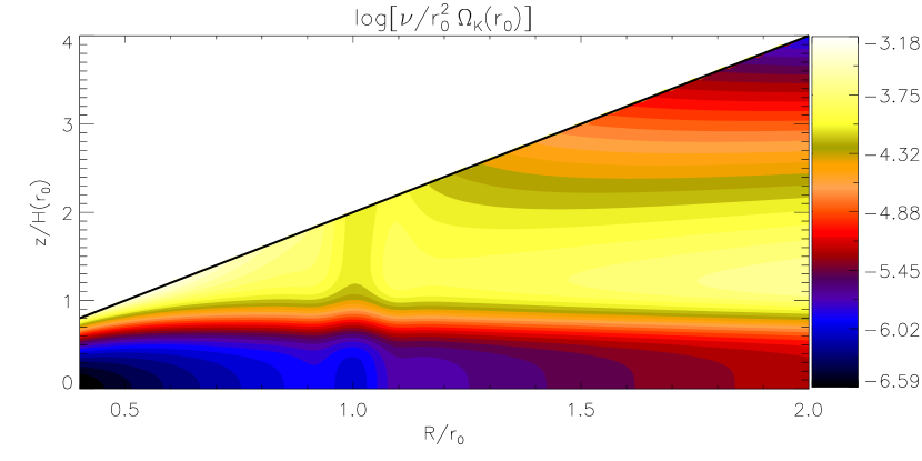
Figure 1: Example of a two-layered kinematic viscosity profile resulting from Eq. 21. This specific plot corresponds to case V2. The solid line delineates the upper boundary of the computational domain.

4.2 Simulations

We consider discs with radial extent $[r_{\mathrm{in}},r_{\mathrm{out}}]=[0.4,2.0]r_{0}$, vertical extent $n_{h}=2$ scale-heights and aspect-ratio $h=0.1$ at $R=r_{0}$. We use $(N_{r},N_{\theta},N_{\phi})=(256,64,512)$ grid points. The resolution at the reference radius is then $16,\,32,\,8$ cells per scale-height in $(r,\theta,\phi)$ directions, respectively. The planet potential is disabled for these runs ($M_{p}\equiv 0$). We apply a damping rate $\hat{\gamma}=1$ with the reference velocity $\bm{v}_{\mathrm{ref}}=\bm{v}(t=0)$.

The bump parameters are set to $A=1.25$ and $\Delta R=0.05r_{0}$ for all runs in this section. The corresponding PV profile is shown in Fig. 2. The spherical radial velocity is subject to random perturbations of magnitude $10^{-4}c_{s}$ a few time-steps after initialization.

Figure 2: Potential vorticity profile for simulations initialised with a surface density bump, as described by Eq. 10. The RWI is associated with the local PV minima at unit radius.

4.2.1 Linear growth rates and frequencies

The present setup allows us to define a linear instability in the usual way: exponential growth of perturbations measured with respect to an axisymmetric steady equilibrium. A proper linear stability analysis, including the full viscous stress tensor, is beyond the scope of this paper, but we can nevertheless extract linear mode frequencies from the non-linear simulations.

The $m^{\mathrm{th}}$ Fourier component of the density field is

$$\hat{\rho}_{m}(r,\theta,t)\equiv\int_{0}^{2\pi}\rho(\bm{r},t)\exp{(-\mathrm{i}m\phi)}d\phi.$$ (23)

The magnitude of a Fourier mode is measured by

$$a_{m}(t)\equiv\frac{b_{m}(t)}{b_{0}(0)},\quad b_{m}(t)\equiv\langle|\hat{\rho}_{m}|\rangle_{r},$$ (24)

where $\langle\cdot\rangle_{r}$ denotes averaging over a spherical shell (to be chosen later). The complex frequency $\sigma_{m}$ associated with the $m^{\mathrm{th}}$ component is defined through

$$\frac{\partial\hat{\rho}_{m}}{\partial t}\equiv-\mathrm{i}\sigma_{m}\hat{\rho}_{m}.$$ (25)

The time derivative in Eq. 25 can be computed implicitly by Fourier-transforming the continuity equation (as done in Lin, 2013b).

In a linear stability problem $\sigma_{m}$ is a constant eigenvalue. However, when extracted numerically from a non-linear simulation, we will generally obtain $\sigma_{m}=\sigma_{m}(r,\theta,t)$. Thus, we compute $\langle\sigma_{m}\rangle_{r}=m\omega_{m}+\mathrm{i}q_{m}$ where $\omega_{m}$ is the mode frequency and $q_{m}$ is the growth rate. We normalize the linear frequencies by $\Omega_{0}\equiv\Omega_{i}(r_{0})\simeq\Omega_{k}(r_{0})$.

4.3 Results

Table 1 summarizes the simulations presented in this section. For reference we simulate an effectively inviscid disc, case B0, with the viscosity parameters $\hat{\nu}_{0}=10^{-9}$ and $A_{\nu}=1$. Thus viscosity is independent of $z$ at $R=r_{0}$. Inviscid setups similar to case B0 have previously been simulated both in the linear and non-linear regimes (Meheut et al., 2012b; Lin, 2013b).

We then simulate discs with floor viscosity $\hat{\nu}_{0}=10^{-6}$. The control run case V0 has $A_{\nu}=1$. Thus, case V0 is the viscous version of case B0. We then consider models where the kinematic viscosity increases by a factor $A_{\nu}=100$ for $z>\zeta_{\nu}H_{0}$ at the bump radius. We choose $\zeta_{\nu}=1.5,\,1.0$ for cases V1 and V2, respectively. This gives a upper viscous layer of thickness $0.5H$ and $H$ at $R=r_{0}$. (See Fig. 1 for a plot of the kinematic viscosity profile for case V2.) For case V1 and V2 the transition thickness is fixed to $\Delta\zeta_{\nu}=0.2$. Finally, we consider a high viscosity run, case V3, with $\hat{\nu}_{0}=10^{-4}$ and $A_{\nu}=1$. This is equivalent to extending the viscous layer in case V1/V2 to the entire vertical domain.

Table 1: Summary of hydrodynamic simulations initialized with a density bump. Linear mode frequencies and the non-linear mode amplitudes $a_{m}$ are averaged over $r\in[0.8,1.2]r_{0}$.

				$t=10P_{0}$ (linear phase)			$t=100P_{0}$
Case	$\log{\hat{\nu}_{0}}$	$A_{\nu}$	$\zeta_{\nu}$	$m$	$\omega_{m}/\Omega_{0}$	$q_{m}/\Omega_{0}$	$m$	$10^{2}a_{m}$	$\mathrm{min}[Ro(z=0)]$
B0	-9	1	n/a	4	0.985	0.199	1	8.5	-0.15
V0	-6	1	n/a	4	0.985	0.199	1	6.8	-0.11
V1	-6	100	1.5	4	0.986	0.191	1	7.8	-0.19
V2	-6	100	1.0	4	0.986	0.182	1	4.9	-0.21
V3	-4	1	n/a	4	0.986	0.131	3	3.7	-0.25

4.3.1 Inviscid reference case

Fig. 3 shows the density fluctuation and Rossby number for case B0. The dominant linear mode is $m=4$ with a growth rate $0.2\Omega_{0}$, consistent with recent 3D linear calculations (Meheut et al., 2012b; Lin, 2013b). The non-linear outcome of the RWI is vortex formation (Li et al., 2000). Four vortices develop initially, then merge on a dynamical timescale into a single vortex. Case B0 evolves similarly to previous simulations of the RWI in an inviscid disc (e.g. Meheut et al., 2010, 2012a, where more detailed analyses are given). This, together with the agreement with linear calculations, demonstrates the ability of the PLUTO code to capture the RWI.

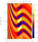
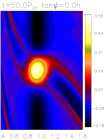
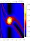
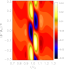
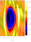
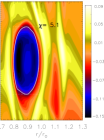
Figure 3: Evolution of the inviscid case B0. Top: midplane density fluctuation, $\Delta\rho(z=0)$. Bottom: midplane Rossby number (note the different axis range from the top panel). Here, $\chi$ is an empirical measure of the final vortex aspect-ratio. $\phi_{0}$ is the azimuth of $\mathrm{max}\left[|\Delta\rho(z=0)|\right]$.

4.3.2 The effect of a viscous layer

We now examine viscous cases V0 — V3. Recall from Table 1 that the viscous layer (with $\hat{\nu}\sim 10^{-4}$) occupies the uppermost $0\%,\,25\%,\,50\%$ and $100\%$ of the vertical domain at $R=r_{0}$ for cases V0, V1, V2 and V3, respectively.

We first compare the viscous case V0 to the inviscid case B0. Table 1 shows that despite increasing the viscosity by a factor of $10^{3}$, the change to the linear mode frequencies are negligible. The value of $a_{m}$ and minimum Rossby number indicate that the final vortex in V0 is only slightly weaker than that in B0. This is also reflected in Fig. 3 (case B0) and the leftmost column in Fig. 4 (case V0). Case V0 develops a more elongated vortex with smaller $|\Delta\rho|$ than that in B0.

As we introduce and thicken the viscous layer from case V0 to V3, the dominant linear mode remains at $m=4$ (Table 1), but linear growth rate does appreciably decrease (by $\sim 34\%$ from case V0 to V3). However, these linear growth timescales are still $\sim P_{0}$. We thus have the important result that viscosity (layered or not) does not significantly affect the linear instability because the RWI grows dynamically even in the high viscosity disc.

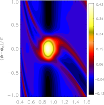
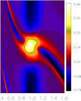
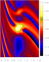
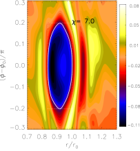
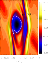
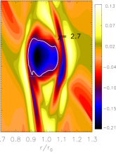
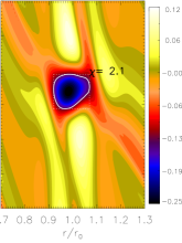
Figure 4: Vortex formation in viscous discs initialised with a density bump at unit radius. Snapshots are taken at $t=100P_{0}$. The thickness of the viscous layer increases from left to right: case V0, V1, V2 and V3. Top: non-axisymmetric density field at the midplane $\Delta\rho(z=0)$. Bottom: midplane Rossby number $Ro(z=0)$. Here, $\phi_{0}$ is the azimuth of $\max[\Delta\rho(z=0)]$.

The effect of layered viscosity in the non-linear regime is more complicated. The bottom row of Fig. 4 compares the Rossby number associated with the over-densities. Thickening the viscous layer decreases the vortex aspect ratio. Since their widths remain at $\sim 2H_{0}$, the vortices become smaller with increasing viscosity. This is partly attributed to fewer vortex merging events having occurred as viscosity is increased, which usually results in larger but weaker vortices (smaller $|Ro|$). If merging is resisted then each vortex can grow individually. Strangely, vortices become stronger (more negative $Ro$) as viscosity is increased.

Fig. 5 compares the perturbed kinetic energy for cases B0, V0 and V1; which are all dominated by a single vortex in quasi-steady state. We compute $W_{1}$ and compare its average over the disc atmosphere and over the disc bulk. There is only a minor difference between the perturbed kinetic energy densities between the disc bulk and atmosphere, even in case V1 where the kinematic viscosity in the two regions differ by a factor $\sim 10^{2}$. This suggests that the vortex evolves two-dimensionally.

The energy perturbation in case B0 and V0 are both subject to slow decay (a result also observed by Meheut et al., 2012b). By contrast case V1, which includes a high viscosity layer, does not show such a decay. We discuss this counter-intuitive result below.

Figure 5: The $m=1$ component of the kinetic energy density, averaged over $r\in[0.8,1.2]r_{0}$, for the inviscid case B0 (solid), low viscosity case V0 (dotted) and a layered viscosity case V1 (dashed). For each, the contribution averaged over the disc atmosphere ($\tan{\psi}\in[1.5,2.0]h$, thin lines) and over the disc bulk ($\tan{\psi}\in[0,1.5]h$, thick lines) are plotted separately.

4.4 Order of magnitude comparison of timescales

The characteristic spatial scale of the background density bump and of the RWI is the local scale-height $H$, so the associated viscous timescale is

$$t_{\nu}=\frac{H^{2}}{\nu}\sim\frac{h^{2}}{\hat{\nu}\Omega}.$$ (26)

The linear instability growth timescale is

$$t_{\mathrm{RWI}}=\frac{1}{\epsilon\Omega},$$ (27)

where $\epsilon$ is found from numerical simulations. The ratio of these timescales is

$$\frac{t_{\nu}}{t_{\mathrm{RWI}}}\sim\frac{\epsilon h^{2}}{\hat{\nu}}.$$ (28)

Table 1 indicates $\epsilon\sim 0.1$. Inserting $h=0.1$ and $\hat{\nu}=10^{-4}$ gives $t_{\nu}\sim 10t_{\mathrm{RWI}}$. Thus viscosity damping is slower than linear growth, even for the highest viscosity values we consider. Consequently the linear RWI is unaffected by viscosity.

Meheut et al. (2013) argued that $t_{\mathrm{RWI}}$ is also the vortex turn-over time $t_{\mathrm{turn}}$ when the instability saturates and the linear phase terminates. Then $t_{\nu}\sim 10t_{\mathrm{turn}}$, implying viscous effects are unimportant over one turn-over time. However, if we estimate a vortex turn-over time as $t_{\mathrm{turn}}\sim 2\pi/|Ro|\Omega$ then $t_{\nu}\sim(h^{2}|Ro|/2\pi\hat{\nu})t_{\mathrm{turn}}$. Inserting $h=0.1,\,\hat{\nu}=10^{-4}$ and $|Ro|=0.25$ (case V3) gives $t_{\nu}\sim 4t_{\mathrm{turn}}$. Therefore, depending on the vortex shape, $t_{\nu}$ may not be much larger than $t_{\mathrm{turn}}$.

In any case, our high-viscosity simulations span several local viscous timescales, $t_{\mathrm{sim}}\sim 10t_{\nu}$ (for $\hat{\nu}\sim 10^{-4}$), so viscous damping should have taken place, making the observation that $Ro$ becomes more negative as the viscous layer increases from case V0 to V3, a surprising result. However, recall that we imposed a stationary, radially structured viscosity profile consistent with a steady-state disc containing a density bump. We suggest that for such setups, viscosity attempts to restore the initial disc profile, i.e. the initial PV minimum, thereby acting as a vorticity source.

4.5 Potential vorticity evolution

The RWI is stronger for deeper PV minima (Li et al., 2000). We thus expect deeper PV minima to correlate with stronger vortices. For the above simulations the axisymmetric PV perturbation at the bump radius is

$$\left.\frac{\langle\eta_{z}\rangle_{\phi}(t=100P_{0})}{\eta_{z}(t=0)}\right|_{R=r_{0}}-1=\begin{cases}3.99&\text{Case V0}\\ 3.03&\text{Case V1}\\ 2.24&\text{Case V2}\\ 1.71&\text{Case V3}\\ \end{cases}.$$ (29)

(This value is 4.92 for the inviscid case B0.) The PV perturbation is positive, thus the initial PV minimum is weakened by the vortices (Meheut et al., 2010). This effect diminishes with increasing viscosity. One contributing factor is the reduction in linear growth rate (Table 1), implying the instability saturates at a smaller amplitude (Meheut et al., 2013). This is expected to weaken the background axisymmetric structure to a lesser extent. However, the imposed viscosity profile may also actively restore the initial density bump.

When viscosity is small, the local viscous timescale $t_{\nu}$ is long compared to our simulation timescale $t_{\mathrm{sim}}$. Then vortex formation weakens the PV minimum with viscosity playing no role. Increasing viscosity eventually makes $t_{\nu}<t_{\mathrm{sim}}$. This means that over the course of the simulation, our spatially-fixed viscosity profile can act to recover the initial PV minimum.

We also notice reduced vortex migration in Fig. 4 with increased viscosity (e.g. the vortex in case V0 has migrated inwards to $R\simeq 0.9r_{0}$ while that in case V3 remains near $R\simeq r_{0}$). Paardekooper et al. (2010) have shown that vortex migration can be halted by a surface density bump which, in our case, can be sourced by the radially-structured viscosity profile.

We conjecture that in the non-linear regime there is competition between destruction of the background PV minimum by the vortices and reformation of the initial radial PV minimum by the imposed viscosity profile. The latter effect should favour the RWI, since the anti-cyclonic vortices are regions of local vorticity minima. In this way, viscosity acts to source vorticity, and this effect outweighs viscous damping of the linear perturbations. We discuss additional simulations supporting this hypothesis in Appendix A.

5 Vortex formation at planetary gap edges in layered discs

The previous simulations, while necessary to isolate the effect of viscosity on the linear RWI, has the disadvantage that the radially structured viscosity profile can act to source radial disc structure in the non-linear regime. In this section, we employ a radially smooth viscosity profile and use disc-planet interaction to create the disc structure required for instability. Then we expect viscosity to only act as a damping mechanism.

Vortex formation at gap edges is a standard result in 2D and 3D hydrodynamical simulations of giant planets in low viscosity discs (de Val-Borro et al., 2007; Lin & Papaloizou, 2010, 2011; Lin, 2012a; Zhu et al., 2013). The fact that this is due to the RWI has been explicitly verified through linear stability analysis (de Val-Borro et al., 2007; Lin & Papaloizou, 2010). Here, we simulate gap-opening giant planets in 3D discs where the kinematic viscosity varies with height above the disc midplane. Our numerical setup is similar to those that in Pierens & Nelson (2010), but our interest is gap stability in a layered disc.

5.1 Radially smooth viscosity profile for disc-planet interaction

Using the same notation as §4.1.2, we impose a viscosity profile $\hat{\nu}$ such that

$$\hat{\nu}\Sigma_{i}(R)=\hat{\nu}_{0}\left[1+Q(\psi)\right]\Sigma_{i}(r_{0})$$ (30)

We have set the dimensionless argument in Eq. 22 to $\zeta=\psi$. Recall $\psi=\pi/2-\theta$ is the angular height away from the midplane. Viscosity increases from its floor value $\hat{\nu}_{0}$ by a factor $A_{\nu}$ for $\psi>\zeta_{\nu}$. So the viscous layer is a wedge in the meridional plane, which conveniently fits into our spherical grid. The angular thickness of the viscosity transition is fixed to $\Delta\zeta_{\nu}=0.2h$. Fig. 6 gives an example of this viscosity profile.

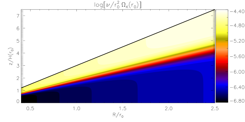
Figure 6: Example of the viscosity profile imposed in disc-planet simulations (Eq. 30). For a disc with constant aspect ratio, the viscous layer occupies a constant number of scale heights across the radial range. This specific plot corresponds to case P1, so the viscous layer (yellow-white colours) always occupies the uppermost $H$ at each cylindrical radius. The solid line delineates the upper boundary of the computational domain.

5.2 Disc-planet simulations

We simulate locally isothermal discs with constant aspect-ratio $h=0.05$ (by choosing $q=1$), vertical extent $n_{h}=3$ scale-heights and radial extent $[r_{\mathrm{in}},r_{\mathrm{out}}]=[0.4,2.5]r_{0}$. Initially the surface density is smooth ($A=1$) with zero meridional velocity ($v_{r}=v_{\theta}=0$). The standard resolution is $(N_{r},N_{\theta},N_{\phi})=(256,96,768)$, corresponding to $6,\,32,\,6$ cells per $H$ along the $r,\theta,\phi$ directions at the reference radius. We apply a damping rate $\hat{\gamma}=2$ with the reference velocity field $\bm{v}_{\mathrm{ref}}=(0,0,v_{\phi})$ in spherical co-ordinates.

We insert into the disc a planet of mass $M_{p}=10^{-3}M_{*}$, which corresponds to a Jupiter mass planet if $M_{*}=M_{\sun}$. The softening length for the planet potential is $\epsilon_{p}=0.5r_{h}$. The planet potential is switched on smoothly over $t\in[0,10]P_{0}$. We note that the disc can be considered as two-dimensional for gap-opening giant planets, because the Hill radius $r_{h}$ exceeds the local scale-height $H$ ($r_{h}/H\simeq 1.4$ in our cases). Fig. 7 shows a typical PV profile associated with the gap induced by the planet.

We remark that, apart from the viscosity prescription, the above choice of physical and numerical parameter values are typical for global disc-planet simulations (e.g. de Val-Borro et al., 2006; Mignone et al., 2012).

Figure 7: Potential vorticity profile for a planet gap before it becomes unstable (case P0). The planet is located at $R=r_{0}$ and the RWI first develops at the PV minima near the outer gap edge at $R\simeq 1.2r_{0}$.

5.3 Results

Table 2 summarizes the disc-planet simulations. The main simulations to be discussed are cases P0 — P1, with a floor viscosity of $\hat{\nu}_{0}=2.5\times 10^{-7}$. The fiducial run P0 has $A_{\nu}=1$, i.e. no viscous layer, so that $\alpha\sim 10^{-4}$ everywhere. The more typical viscosity value adopted for disc-planet simulations, $\hat{\nu}\sim 10^{-5}$ or $\alpha\sim 10^{-3}$, is known to suppress vortex formation (de Val-Borro et al., 2007; Mudryk & Murray, 2009). Thus vortex formation is expected in case P0. For case P0.5 and P1 we set $A_{\nu}=100$ with transition angle $\zeta_{\nu}=2.5h$ and $2h$, respectively, so the viscous layer with $\alpha\sim 10^{-2}$ occupies the uppermost $0.5H$ and $H$ of the vertical domain. Case P0R is case P0 restarted from $t=100P_{0}$ with the layered viscosity profile of case P1.

Table 2: Summary of disc-planet simulations. These runs employ the ‘wedge’ viscosity model described by Eq. 30. The thickness of the viscous layer is measured from the upper disc boundary. The $m=1$ mode amplitude was averaged over the shell $r\in[1.2,1.6]r_{0}$; and the overbar denotes a further time average over $t\in[t_{\mathrm{max}},200]P_{0}$, where $t_{\mathrm{max}}$ is when $\mathrm{max}(a_{1})$ is attained. Case P0R employs the viscosity profile of P0 for $t\leq 100P_{0}$, and that of P1 for $t>100P_{0}$.

Case	$10^{6}\hat{\nu}_{0}$	$A_{\nu}$	visc. layer	$10^{2}\overline{a}_{1}$	$10^{2}a_{1}(200P_{0})$	comment
P0	0.25	1	0	18.3	14.5	single vortex by $t=130P_{0}$ and persists until end of sim.
P0.5	0.25	100	$0.5H$	17.4	8.6	single vortex by $t=90P_{0}$ and persists until end of sim.
P0R	0.25	1$\to$100	$0\to H$	10.1	2.5	single vortex by $t=130P_{0}$, disappears after $t=180P_{0}$
P1	0.25	100	$H$	12.5	2.1	single vortex by $t=80P_{0}$, disappears after $t=170P_{0}$
Pb0	1.0	1	0	9.2	5.4	single vortex by $t=130P_{0}$, disappears after $t=160P_{0}$
Pb0.5	1.0	10	$0.5H$	7.3	3.0	similar to Pb0
Pb1	1.0	10	$H$	5.7	2.2	single vortex by $t=120P_{0}$, disappears after $t=140P_{0}$
Pc0.5	1.0	100	$0.5H$	4.2	2.3	two vortices at $t\sim 100P_{0}$, no vortices after $t\sim 120P_{0}$
Pc1	1.0	100	$H$	2.2	1.6	two weak vortices at $t\sim 60P_{0}$, no vortices after $t\sim 80P_{0}$

5.3.1 Density evolution

Fig. 8 compares the time evolution of the midplane density perturbation $\delta\rho(z=0)$ for cases P0, P0.5 and P1. In all cases we observed the RWI with $m=4$ develops early on ($t\simeq 20P_{0}$), consistent with the limited effect of viscosity on the linear instability, as found above. The no-layer case P0 and layered case P0.5 (viscous layer of $0.5H$) behave similarly, showing that a thin viscous layer has little effect on the evolution of the unstable gap edge, at least over the simulation time-scale of $200P_{0}$.

Case P1 evolves quite differently from case P0. While a single vortex does form at $t\sim 100P_{0}$, it is transient, having disappeared at the end of the simulation for P1. The final $m=1$ amplitude is about 3 times smaller than that in case P0 (Table 2). This result is significant because the upper viscous layer in case P1, of thickness $H$, only occupies $\sim 4\%$ of the total column density, but the vortex is still destroyed. This suggests that vortex survival at planetary gap edges requires low effective viscosity throughout the vertical fluid column.

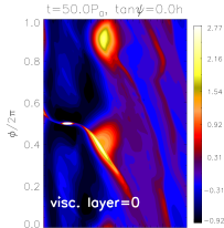
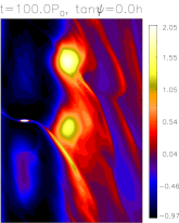
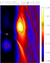
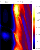
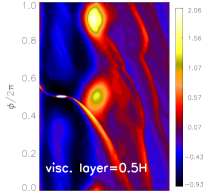
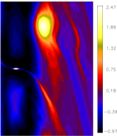
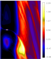
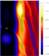
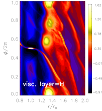
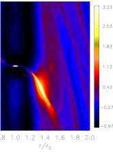
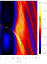
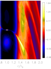
Figure 8: Relative density perturbation $\delta\rho$ for disc-planet simulations. Top: case P0 (no viscous layer), middle: case P0.5 (viscous layer of $0.5H$), bottom: case P1 (viscous layer of $H$). The vertical extent of the computational domain is $3H$ and the viscous layer is measured from the upper disc boundary.

5.3.2 Kinetic energy density

Here, we compare the $m=1$ component of the kinetic energy density ($W_{1}$) between the no-layer case P0, layered case P1 and case P0R which is P0 resumed from $t=100P_{0}$ with a viscous layer. Fig. 9 shows $W_{1}(t)$ averaged over the outer gap edge. For each case we average $W_{1}$ over the disc bulk and the atmosphere, and plot them separately in the figure.

The $m=1$ component does not emerge from the linear instability, but is a result of non-linear vortex merging. Fig. 9 shows that merging is accelerated by a viscous layer: the single vortex appears at $t\sim 70P_{0}$ for case P1 but only forms at $t\sim 120P_{0}$ for case P0. Also note for all cases, $W_{1}$ in the disc bulk (thick lines) is similar to that in the disc atmosphere (thin lines), implying the $m=1$ disturbance (i.e. the vortex) evolves two-dimensionally. We checked that this is consistent with the Froude number $Fr\equiv|Ro|H/z<1$ away from the midplane (Barranco & Marcus, 2005; Oishi & Mac Low, 2009).

Case P0R shows that introducing a viscous layer eventually destroys the vortex. The local viscous timescale is $t_{\nu}\equiv H^{2}/\nu\;\raisebox{-3.44444pt}{$\buildrel\textstyle>\over{\sim}$}\;16P_{0}$, so on short timescales after introducing the viscous layer ($t=100P_{0}$), vortex-merging proceeds in case P0R similarly to case P0 ($t\in[100,110]P_{0}$). However, $W_{1}$ decays for $t>110P_{0}$ and evolves towards that of case P1. We expect viscosity to damp the $m=1$ disturbance in the disc atmosphere between $t\in[110,200]P_{0}$ because this corresponds to $\sim 6t_{\nu}$, but the disturbance in the disc bulk is also damped out: the evolution remains two-dimensional.

Figure 9: Evolution of the $m=1$ component of kinetic energy density, averaged over $r\in[1.2,1.6]r_{0}$. This average is split into that taken over disc bulk ($z\in[0,2]H$, thick lines) and the disc atmosphere ($z\in[2,3]H$, thin lines). Case P0 has no viscous layer (solid) and case P1 has a viscous layer in $z\in[2,3]H$ (dashed). Case P0R (dotted) is identical to P0 up to $t=100P_{0}$, but was simulated for $t>100P_{0}$ with a viscous layer of thickness $H$.

We emphasize the kinetic energy is dominated by horizontal motions, with $\mathrm{max}(|v_{z}|/|\bm{v}|)<0.03$ at the outer gap edge ($r\in[1.2,1.6]r_{0}$). Vertical motions are well sub-sonic. When averaged over $z\in[0,2]H$ and $z\in[2,3]H$, the vertical Mach number $M_{z}\equiv|v_{z}|/c_{s}\simeq 0.05,\,0.08$ (P0), $M_{z}\simeq 0.04,\,0.06$ (P0R) and $M_{z}\simeq 0.05,0.06$ (P1), respectively.

5.3.3 Potential vorticity

We examine the PV evolution for case P0R in Fig. 10. To highlight the vortices, which are positive (negative) density (vertical vorticity) perturbations, we show the inverse PV perturbation, $\delta\eta_{z}^{-1}\equiv\eta_{z}(t=0)/\eta_{z}-1$. As noted above, a single vortex still forms despite introducing a viscous layer at $t=100P_{0}$. However, it decays rapidly compared to case P0. The region with $\delta\eta_{z}^{-1}>0$ (i.e. the vortex) elongates and shifts outward from $R\simeq 1.38r_{0}$ at $t=140P_{0}$ to $R\simeq 1.5r_{0}$ at $t=200P_{0}$, by which the vortex has disappeared. (A similar evolution was observed for case P1.) The vortex is stretched azimuthally much more than radially. This is not surprising since the imposed viscosity profile is axisymmetric. The important point is that viscosity is only large near the disc surface, but still has a significant effect on the vortex.

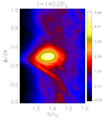
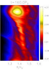
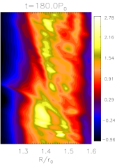
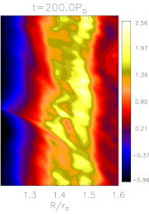
Figure 10: Inverse PV perturbation, $\eta_{z}(t=0)/\eta_{z}-1$, for case P0R, which was resumed from the no-layer case P0 from $t=100P_{0}$ with the introduction of a viscous layer of $H$.

5.3.4 Resolution check

We repeated simulations P0 and P1 with resolution $(N_{r},N_{\theta},N_{\phi})=(512,96,1536)$, corresponding to $12$ and $32$ cells per scale-height in $(r,\phi)$ and $\theta$, respectively. We denote these runs as P0HR and P1HR below.

We observe similar evolution in P0HR and P1HR as their standard resolution versions. However, due to lower numerical diffusion, we find stronger vortices in P0HR. Although the vortex in P1HR persisted longer than the standard resolution run, it was still subject to rapid decay in comparison with P0HR. At $t=200P_{0}$ we find the $m=1$ amplitude to be $a_{1}=0.29$ and $a_{1}=0.10$ at the outer gap edge, respectively for P0HR and P1HR; a similar contrast as that between P0 and P1. A weak over-density was still observed in P1HR at $t=200P_{0}$, but it further decays to $a_{1}=0.06$ at $t=230P_{0}$ and there is no vortex. By contrast, P0HR was simulated to $t=250P_{0}$ and the vortex survived with little decay ($a_{1}=0.25$).

Interestingly, we observe small-scale ($\;\raisebox{-3.44444pt}{$\buildrel\textstyle<\over{\sim}$}\;H$) disturbances inside the vortex in P0HR. This is shown in the left panel of Fig. 11 in terms of the (inverse) PV perturbation. We checked the density field remains smooth, so this small-scale structure is due to vorticity variations. This is unlikely the elliptic instability (Lesur & Papaloizou, 2009), though, because the numerical resolution is still insufficient for studying such instabilities; especially since the vortex is very elongated with large aspect ratio $\sim 10$ (so the elliptic instability is weak, Lesur & Papaloizou, 2009). Despite the disturbances, the vortex over-density in P0HR remains coherent until the end of the simulation, possibly because the planet maintains the condition for RWI. On the other hand, the vortex in the layered-case P1HR does not develop small-scale structure (Fig. 11, right panel), yet it is destroyed by the end of the simulation.

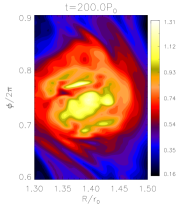
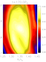
Figure 11: Logarithmic inverse PV perturbation associated with a vortex, $\log{\left[\eta_{z}(t=0)/\eta_{z}\right]}$, for high resolution cases P0HR (left, no viscous layer) and P1HR (right, with a viscous layer). These cases are the same as P0 and P1, but with double the $(r,\phi)$ resolution. The vortex in P1HR (right) eventually disappears after $t\sim 200P_{0}$.

5.4 Additional simulations

Locally isothermal, low viscosity discs are vulnerable to the so-called ‘vertical shear instability’ because $\partial_{z}\Omega_{i}\neq 0$ (Nelson et al., 2013). Nelson et al. employed a radial resolution $\;\raisebox{-3.44444pt}{$\buildrel\textstyle>\over{\sim}$}\;60$ cells per $H$ to resolve this instability because it involves small radial wavelengths ($\ll H$). Our numerical resolution is unlikely to capture this instability. Nevertheless, we have performed additional simulations designed to eliminate the vertical shear instability.

5.4.1 Larger floor viscosity

We performed several simulations with $\hat{\nu}_{0}=10^{-6}$. A viscosity of $\hat{\nu}\sim 10^{-6}$ is expected to damp the vertical shear instability (Nelson et al., 2013), while still permitting the gap-edge RWI. Table 2 summarizes these cases with $A_{\nu}=10$ (‘Pb’ runs) and $A_{\nu}=100$ (‘Pc’ runs).

In these simulations we find vortices eventually decay, even in the no-layer case Pb0. For $A_{\nu}=10$, the layered cases Pb0.5 and Pb1 evolve similarly to Pb0: three vortices formed by $t\sim 30P_{0}$, merging into two vortices by $t\sim 40P_{0}$, then finally into a single vortex by $t\sim 130P_{0}$, which subsequently decays. However, the final vortex decays faster in the presence of a viscous layer. This is shown in Fig. 12, which compares the $m=1$ kinetic energy density for case Pb0 and Pb1. The evolution only begins to differ after the single-vortex has formed.

Figure 12: Same as Fig. 9 but with floor viscosity $\hat{\nu}_{0}=10^{-6}$: cases Pb0 (solid, no viscous layer) and Pb1 (dotted, viscous layer of $H$). The thick (thin) lines indicate $W_{1}$ averaged over $z\in[0,2]H$ ($z\in[2,3]H$).

For $A_{\nu}=100$ (cases Pc0.5 and Pc1), we find the $m=2$ amplitude dominated over $m=1$, so a single-vortex configuration never forms. For both Pc0.5 and Pc1 the $m=2$ (two-vortex configuration) amplitude decreases from $t\sim 50P_{0}$. For case Pc1, the vortices are transient features and are entirely absent for $t\;\raisebox{-3.44444pt}{$\buildrel\textstyle>\over{\sim}$}\;80P_{0}$.

5.4.2 Strictly isothermal discs

We repeated simulations Pb0, Pb1 and Pc1 with a strictly isothermal equation of state ($q=0$). These are summarised in Table 3. Fig. 13 compares their $m=1$ kinetic energy density evolution at the outer gap edge. Consistent with the above simulations, a viscous layer causes a faster decay in this quantity. Most interesting though, is that we found case Iso2 (with a viscous layer of $\sim H$) only shows very weak non-axisymmetric perturbations early on ($t\;\raisebox{-3.44444pt}{$\buildrel\textstyle<\over{\sim}$}\;50P_{0}$): vortex formation is suppressed.

Table 3: Disc-planet simulations with a strictly isothermal equation of state ($q=0$). The thickness of the viscous layer is quoted at the reference radius $R=r_{0}$.

Case	$10^{6}\hat{\nu}_{0}$	$A_{\nu}$	visc. layer	$10^{2}\overline{a}_{1}$	vortex
Iso0	1.0	1	0	19.3	YES
Iso1	1.0	10	$H_{0}$	12.8	YES
Iso2	1.0	100	$H_{0}$	1.1	NO

Figure 13: Same as Fig. 9 but for strictly isothermal Iso0 (solid, no viscous layer so $\hat{\nu}\sim 10^{-6}$), Iso1 (dotted, viscous layer with $\hat{\nu}\sim 10^{-5}$) and Iso2 (dashed, viscous layer with $\hat{\nu}\sim 10^{-4}$). The thick (thin) lines indicate $W_{1}$ averaged over $\tan{\psi}\in[0,2]h$ ($\tan{\psi}\in[2,3]h$).

6 Summary and discussion

We have performed customised hydrodynamic simulations of non-axisymmetric instabilities in 3D viscous discs. We adopted height-dependent kinematic viscosity profiles, such that the disc midplane is of low viscosity ($\alpha\sim 10^{-4}$) and the disc atmosphere is of high viscosity ($\alpha\sim 10^{-2}$). We were motivated by the question of whether or not the Rossby wave instability, and subsequent vortex formation, operates in layered accretion discs.

We first considered viscous disc equilibria with a radial density bump and varied the vertical dependence of viscosity. This setup can isolate the effect of viscosity on the linear RWI. We found that the linear RWI is unaffected by viscosity, layered or not. The viscous RWI remains dynamical and leads to vortex formation on timescales of a few 10s of orbits. We continued these simulations into the non-linear regime, but found that vortices became stronger as the viscous layer is increased in thickness. We suggest this counter-intuitive result is an artifact of the chosen viscosity profile because it is radially structured: viscosity attempts to restore the equilibrium radial density bump, which favours the RWI. This effect outweighs viscosity damping the linear instability.

We also simulated vortex formation at planetary gap edges in layered discs with a radially-smooth viscosity profile. Although vortex formation still occurs in layered discs, we found the vortex can be destroyed even when the viscous layer only occupies the uppermost scale-height of the vertical domain which is 3 scale-heights. This is significant because most of the disc mass is contained within 2 scale-heights (i.e. the low viscosity layer) but simulations show a viscous atmosphere inhibits long term vortex survival. We found that the non-axisymmetric energy densities have weak vertical dependence, so the disturbance evolves two-dimensionally. It appears that applying a large viscosity in the disc atmosphere is sufficient to damp the instability throughout the vertical column of the fluid.

Barranco & Marcus (2005) have described two 3D vortex models: tall columnar vortices and short finite-height vortices. Rossby vortices are columnar, i.e. the associated vortex lines extend vertically throughout the fluid column. One might have expected an upper viscous layer to damp out vortex motion in the disc atmosphere, leading to a shorter vortex. This, however, requires vortex lines to loop around the vortex (the short vortex of Barranco & Marcus). Such vortex loops form the surface of a torus (see, for example, Fig. 1 in Barranco & Marcus, 2005), instead of ending on vertical boundaries. This implies significant vertical motion near the vertical boundaries of the vortex, which would be difficult in our model because of viscous damping applied there. We suspect this is why short/tall vortices fail to form/survive in our layered disc-planet models. We conclude that vortex survival at planetary gap edges require low viscosity ($\alpha\;\raisebox{-3.44444pt}{$\buildrel\textstyle<\over{\sim}$}\;10^{-4}$) throughout the vertical extent of the disc.

6.1 Relation to other works

Pierens & Nelson (2010) simulated the orbital migration of giant planets in layered discs by prescribing a height-dependent viscosity profile. They considered significant reduction in kinematic viscosity in going from the disc atmosphere (the active zone, with $\alpha\sim 10^{-2}$) to the disc midplane (the dead zone, with $\alpha\sim 10^{-7}$). According to previous 2D simulations, such a low kinematic viscosity should lead to the RWI (de Val-Borro et al., 2006, 2007). However, Pierens & Nelson (2010) did not report vortex formation, nor are vortices visible from their plots. Very recent MHD simulations of giant planets in a layered disc also did not yield vortex formation (Gressel et al., 2013). These results are consistent with our simulations.

Oishi & Mac Low (2009) carried out MHD shearing box simulations with a resistivity profile that varied with height to model a layered disc: the disc atmosphere was MHD turbulent while the disc midplane remained stable against the MRI. They envisioned the active zone as a vorticity source for vortex formation in the midplane. Although their setup is fundamentally different to ours, they also reported a lack of coherent vortices in the dead zone. They argued that the MHD turbulence in the active layer was not sufficiently strong to induce vortex formation in the dead zone. If MHD turbulence can be represented by a viscosity, the lack of tall columnar vortices in Oishi & Mac Low (2009) is consistent with our results. That is, even when MRI turbulence is only present in the disc atmosphere it is able to damp out columnar vortices.

6.2 Caveats and outlooks

The most important caveat of the current model is the viscous prescription to mimic MRI turbulence. In doing so, an implicit averaging is assumed (Balbus & Papaloizou, 1999). The spatial averaging should be taken on length scales no less than the local disc scale-height, and the temporal average taken on timescales no less than the local orbital period. These are, however, the relevant scales for vortex formation via the RWI. Furthermore, our viscosity profile varies on length-scales comparable to or even less than $H$ (e.g. the vertical transition between high and low viscosity layers). Nevertheless, our simulations demonstrate the importance of disc vertical structure on the RWI. That is, damping, even confined to the disc atmosphere, can destroy Rossby vortices.

Another drawback of a hydrodynamic viscous disc model is the fact that it cannot mimic magneto-elliptic instabilities (MEI), which are known to destroy vortices in magnetic discs (Lyra & Klahr, 2011; Mizerski & Lyra, 2012). A natural question is how Rossby vortices are affected by the MEI when it only operates in the disc atmosphere. Extension of the present work to global non-ideal MHD simulations will be necessary to address RWI vortex formation in layered discs.

However, some improvements can be made within the viscous framework. A static viscosity profile neglects the back-reaction of the density field on the kinematic viscosity. Thus, our simulations only consider how Rossby vortices respond to an externally applied viscous damping. A more physical viscosity prescription should depend on the local column density (Fleming & Stone, 2003), with viscosity decreasing with increasing column density. The effective viscosity inside Rossby vortices would be lowered relative to the background disk because disc vortices are over-densities. If the over-density is large, then it is conceivable that vortex formation itself may render the effective viscosity to be sufficiently low throughout the fluid column to allow long term vortex survival. Preparation for this study is underway and results will be reported in a follow-up paper.

Appendix A Artificial radial density bumps with a radially smooth viscosity profile

In §4 we found that vortices became stronger as the viscous layer thickness is increased, even though linear growth rates were reduced. Here, we present additional simulations to support the hypothesis that this is due to the localised radial structure in the viscosity profile.

We repeated simulation V2 (see Table 1) with a radially-smooth viscosity profile given by

$$\hat{\nu}\frac{\rho_{i}(R,z)}{B(R)}=\hat{\nu}_{0}\left[1+Q(z/H_{0})\right]\frac{\rho_{i}(r_{0},z)}{B(r_{0})}.$$ (31)

Recall the functions $B$ and $Q$ are given by Eq. 10 and 22, respectively. We set the floor viscosity $\hat{\nu}_{0}=10^{-7}$ to mitigate axisymmetric viscous diffusion of the initial density bump. The viscous layer with $\hat{\nu}\sim 10^{-5}$ occupies $z\in[1,2]H_{0}$ at $R=r_{0}$. This viscosity profile is shown in Fig. 14.

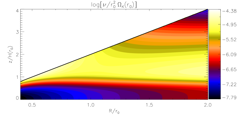
Figure 14: The radially-smooth viscosity profile given by Eq. 31. This plot is to be compared with Fig. 1.

This simulation is shown as the dotted line in Fig. 15 in terms of the $m=1$ component of the kinetic energy density. We compare it to the corresponding case using the radially-structured viscosity profile in §4 (i.e. the original case V2 but with lowered floor viscosity). Vortex formation occurs in both runs. With a radially-smooth viscosity profile, the vortex decays monotonically after $|W_{1}|$ reaches maximum value of $\sim 0.05$. Using the radially-structured viscosity profile (solid line) gives a larger disturbance amplitude at the linear stage ($\max{|W_{1}|}\sim 0.08$), and although it subsequently decays, the decay is halted for $t\;\raisebox{-3.44444pt}{$\buildrel\textstyle>\over{\sim}$}\;110P_{0}$.

The contrast between these cases show that the radial structure in the viscosity profile helps vortex survival. This experiment indicates that the dominant effect of viscosity is its influence on the evolution of the axisymmetric part of background disc. The radially-structured viscosity profile is a source for the radial PV minimum, which is needed for the RWI.

Our result here is qualitatively similar that in Regály et al. (2012), where a sharp viscosity profile was imposed in a 2D simulation and vortex formation ensues via the RWI. The vortex eventually disappears, but re-develops after the system returns to an axisymmetric state. This is because the imposed viscosity profile causes the disc to develop the required PV minimum for the RWI.

Figure 15: Evolution of the $m=1$ component of the kinetic energy density, averaged over the shell $r\in[0.8,1.2]r_{0}$, for a layered disc initialised with a radial density bump. The solid line employs the radially-structured viscosity profile given by Eq. 21 (see Fig.1). The dotted line employs the radially-smooth viscosity profile given by Eq. 31 and shown in Fig. 14.

References

- Armitage (2011) Armitage P. J., 2011, ARAA, 49, 195
- Ataiee et al. (2013) Ataiee S., Pinilla P., Zsom A., Dullemond C. P., Dominik C., Ghanbari J., 2013, A&A, 553, L3
- Balbus & Hawley (1991) Balbus S. A., Hawley J. F., 1991, ApJ, 376, 214
- Balbus & Hawley (1998) Balbus S. A., Hawley J. F., 1998, Reviews of Modern Physics, 70, 1
- Balbus & Papaloizou (1999) Balbus S. A., Papaloizou J. C. B., 1999, ApJ, 521, 650
- Barge & Sommeria (1995) Barge P., Sommeria J., 1995, A&A, 295, L1
- Barranco & Marcus (2005) Barranco J. A., Marcus P. S., 2005, ApJ, 623, 1157
- Bate et al. (2002) Bate M. R., Ogilvie G. I., Lubow S. H., Pringle J. E., 2002, MNRAS, 332, 575
- Birnstiel et al. (2013) Birnstiel T., Dullemond C. P., Pinilla P., 2013, A&A, 550, L8
- Brown et al. (2009) Brown J. M., Blake G. A., Qi C., Dullemond C. P., Wilner D. J., Williams J. P., 2009, ApJ, 704, 496
- de Val-Borro et al. (2007) de Val-Borro M., Artymowicz P., D’Angelo G., Peplinski A., 2007, A&A, 471, 1043
- de Val-Borro et al. (2006) de Val-Borro M. et al., 2006, MNRAS, 370, 529
- Dzyurkevich et al. (2010) Dzyurkevich N., Flock M., Turner N. J., Klahr H., Henning T., 2010, A&A, 515, A70
- Edgar & Quillen (2008) Edgar R. G., Quillen A. C., 2008, MNRAS, 387, 387
- Flaig et al. (2012) Flaig M., Ruoff P., Kley W., Kissmann R., 2012, MNRAS, 420, 2419
- Fleming & Stone (2003) Fleming T., Stone J. M., 2003, ApJ, 585, 908
- Gammie (1996) Gammie C. F., 1996, ApJ, 457, 355
- Gressel et al. (2013) Gressel O., Nelson R. P., Turner N. J., Ziegler U., 2013, ArXiv e-prints
- Inaba & Barge (2006) Inaba S., Barge P., 2006, ApJ, 649, 415
- Isella et al. (2013) Isella A., Pérez L. M., Carpenter J. M., Ricci L., Andrews S., Rosenfeld K., 2013, ApJ, 775, 30
- Koller et al. (2003) Koller J., Li H., Lin D. N. C., 2003, ApJL, 596, L91
- Kretke & Lin (2010) Kretke K. A., Lin D. N. C., 2010, ApJ, 721, 1585
- Landry et al. (2013) Landry R., Dodson-Robinson S. E., Turner N. J., Abram G., 2013, ApJ, 771, 80
- Lesur & Papaloizou (2009) Lesur G., Papaloizou J. C. B., 2009, A&A, 498, 1
- Li et al. (2001) Li H., Colgate S. A., Wendroff B., Liska R., 2001, ApJ, 551, 874
- Li et al. (2000) Li H., Finn J. M., Lovelace R. V. E., Colgate S. A., 2000, ApJ, 533, 1023
- Li et al. (2005) Li H., Li S., Koller J., Wendroff B. B., Liska R., Orban C. M., Liang E. P. T., Lin D. N. C., 2005, ApJ, 624, 1003
- Li et al. (2009) Li H., Lubow S. H., Li S., Lin D. N. C., 2009, ApJL, 690, L52
- Lin (2012a) Lin M.-K., 2012a, ApJ, 754, 21
- Lin (2012b) Lin M.-K., 2012b, MNRAS, 426, 3211
- Lin (2013a) Lin M.-K., 2013a, MNRAS, 428, 190
- Lin (2013b) Lin M.-K., 2013b, ApJ, 765, 84
- Lin & Papaloizou (2010) Lin M.-K., Papaloizou J. C. B., 2010, MNRAS, 405, 1473
- Lin & Papaloizou (2011) Lin M.-K., Papaloizou J. C. B., 2011, MNRAS, 415, 1426
- Lovelace et al. (1999) Lovelace R. V. E., Li H., Colgate S. A., Nelson A. F., 1999, ApJ, 513, 805
- Lynden-Bell & Pringle (1974) Lynden-Bell D., Pringle J. E., 1974, MNRAS, 168, 603
- Lyra et al. (2009) Lyra W., Johansen A., Klahr H., Piskunov N., 2009, A&A, 493, 1125
- Lyra & Klahr (2011) Lyra W., Klahr H., 2011, A&A, 527, A138
- Lyra & Lin (2013) Lyra W., Lin M.-K., 2013, ApJ, 775, 17
- Lyra & Mac Low (2012) Lyra W., Mac Low M.-M., 2012, ApJ, 756, 62
- Masset (2000) Masset F., 2000, A&AS, , 141, 165
- Mayama et al. (2012) Mayama S. et al., 2012, ApJL, 760, L26
- Meheut et al. (2010) Meheut H., Casse F., Varniere P., Tagger M., 2010, A&A, 516, A31
- Meheut et al. (2012a) Meheut H., Keppens R., Casse F., Benz W., 2012a, A&A, 542, A9
- Meheut et al. (2013) Meheut H., Lovelace R. V. E., Lai D., 2013, MNRAS, 430, 1988
- Meheut et al. (2012b) Meheut H., Yu C., Lai D., 2012b, MNRAS, 422, 2399
- Mignone et al. (2007) Mignone A., Bodo G., Massaglia S., Matsakos T., Tesileanu O., Zanni C., Ferrari A., 2007, ApJS, , 170, 228
- Mignone et al. (2012) Mignone A., Flock M., Stute M., Kolb S. M., Muscianisi G., 2012, A&A, 545, A152
- Mizerski & Lyra (2012) Mizerski K. A., Lyra W., 2012, Journal of Fluid Mechanics, 698, 358
- Mudryk & Murray (2009) Mudryk L. R., Murray N. W., 2009, New A, 14, 71
- Nelson et al. (2013) Nelson R. P., Gressel O., Umurhan O. M., 2013, MNRAS
- Oishi & Mac Low (2009) Oishi J. S., Mac Low M.-M., 2009, ApJ, 704, 1239
- Okuzumi & Hirose (2011) Okuzumi S., Hirose S., 2011, ApJ, 742, 65
- Paardekooper et al. (2010) Paardekooper S.-J., Baruteau C., Crida A., Kley W., 2010, MNRAS, 401, 1950
- Pierens & Nelson (2010) Pierens A., Nelson R. P., 2010, A&A, 520, A14
- Regály et al. (2012) Regály Z., Juhász A., Sándor Z., Dullemond C. P., 2012, MNRAS, 419, 1701
- Richard et al. (2013) Richard S., Barge P., Le Dizes S., 2013, ArXiv e-prints
- Shakura & Sunyaev (1973) Shakura N. I., Sunyaev R. A., 1973, A&A, 24, 337
- Takeuchi & Lin (2002) Takeuchi T., Lin D. N. C., 2002, ApJ, 581, 1344
- Terquem (2008) Terquem C. E. J. M. L. J., 2008, ApJ, 689, 532
- Umurhan (2010) Umurhan O. M., 2010, A&A, 521, A25
- van der Marel et al. (2013) van der Marel N. et al., 2013, Science, 340, 1199
- Zhu et al. (2013) Zhu Z., Stone J. M., Rafikov R. R., Bai X., 2013, ArXiv e-prints