The planets around NN Serpentis: still there

Abstract

We present 25 new eclipse times of the white dwarf binary NN Ser taken with the high-speed camera ULTRACAM on the WHT and NTT, the RISE camera on the Liverpool Telescope, and HAWK-I on the VLT to test the two-planet model proposed to explain variations in its eclipse times measured over the last 25 years. The planetary model survives the test with flying colours, correctly predicting a progressive lag in eclipse times of 36 seconds that has set in since 2010 compared to the previous 8 years of precise times. Allowing both orbits to be eccentric, we find orbital periods of $7.9\pm 0.5\,$yr and $15.3\pm 0.3\,$yr, and masses of $2.3\pm 0.5\,\mathrm{M}_{\mathrm{J}}$ and $7.3\pm 0.3\,\mathrm{M}_{\mathrm{J}}$. We also find dynamically long-lived orbits consistent with the data, associated with 2:1 and 5:2 period ratios. The data scatter by $0.07$ seconds relative to the best-fit model, by some margin the most precise of any of the proposed eclipsing compact object planet hosts. Despite the high precision, degeneracy in the orbit fits prevents a significant measurement of a period change of the binary and of $N$-body effects. Finally, we point out a major flaw with a previous dynamical stability analysis of NN Ser, and by extension, with a number of analyses of similar systems.

1 Introduction

The discovery of hundreds of planets around stars other than the Sun has alerted researchers to the possible influence of planets in a wide variety of circumstances. Amongst these are the spectacular Kepler discoveries of planets transiting across both stars of the tighter binary systems around which they orbit (Doyle et al., 2011; Welsh et al., 2012). The transits in these systems leave no doubt as to the existence of planets in so-called “P-type” orbits (Dvorak, 1986) around binaries. Even before the Kepler discoveries there was evidence for planets around binaries from timing observations of a variety of systems where the presence of planets is indicated through light travel time (LTT) induced variations in the times of eclipses. This method has led to claims of planetary and/or sub-stellar companions around hot subdwarf/M dwarf binaries (Lee et al., 2009; Qian et al., 2009b), white dwarf/M dwarf binaries (Qian et al., 2009a, 2010; Beuermann et al., 2010), and cataclysmic variables (Beuermann et al., 2011; Qian et al., 2011; Potter et al., 2011). In all the cases cited one of the binary components is evolved which helps observationally because the evolved star is hot and relatively small, leading to sharply-defined, deep edges in eclipse light curves which make for precise times.

Planets discovered through timing complement those found in radial velocity and transit surveys as they are easier to discover the larger (and thus longer period) their orbits are. The existence of planets around evolved stars raises interesting questions as to whether the planets are primordial and managed to survive the evolution of the host binary, or whether they instead formed from material ejected during the course of stellar evolution (Beuermann et al., 2011; Veras & Tout, 2012; Mustill et al., 2013), and may also place unusual constraints upon the binary’s evolution (Portegies Zwart, 2013).

The Kepler discoveries prove that circumbinary planets exist, but when it comes to those discovered through timing, the reality of the planets is not clear-cut. The history of the field is not encouraging in this respect. For instance, the orbits measured for the white dwarf/M dwarf binaries NN Ser and QS Vir by Qian et al. (2009a) and Qian et al. (2010) were both ruled out as soon as new data were acquired (Parsons et al., 2010b), as were the two-planet orbits proposed by Lee et al. (2009) for the sdB+dM binary HW Vir (Beuermann et al., 2012). Likewise, some multiple planet systems claimed from timing studies (Qian et al., 2011) have had problems with long-term dynamical stability (Horner et al., 2011; Hinse et al., 2012; Potter et al., 2011). These are serious issues because there is no independent evidence yet for the existence of the various third-bodies suggested by timing, while the mere fact that timing variations can be fitted by planetary models is not entirely persuasive, since with enough extra bodies the process is akin to fitting a Fourier series, and any set of data can be matched. At present, the main rival model for the period changes is one in which they are caused by fluctuations in the gravitational quadrupolar moments of one or both stars (Applegate, 1992). In some cases this appears to fail on energetic grounds (Brinkworth et al., 2006), and at the moment this constitutes the only, rather indirect, independent support for the planetary hypothesis for the eclipse timing variations of compact binary stars, although artefacts of measurement, such as wavelength-dependent eclipse timings, are a possible issue in the case of accreting systems (Goździewski et al., 2012).

Useful scientific hypotheses have predictive power. So far the planetary explanation of LTT variations has fared poorly on this basis. In this paper we present new observations of the system NN Ser which is currently the most convincing example of an LTT-discovered planetary system around a close binary star. Our aim is to see whether the planetary model developed by Beuermann et al. (2010) can withstand the test of new data. NN Ser is a white dwarf/M dwarf binary with an orbital period $P=3.1\,$hours which was discovered to eclipse by Haefner (1989). The combination of a hot white dwarf and low mass M dwarf ($0.111\,\mathrm{M}_{\odot}$, Parsons et al. 2010a), allows the white dwarf to dominate its optical flux completely, giving very deep, sharply-defined eclipses which yield precise times. The very low mass of the M dwarf is an important feature since its low luminosity greatly restricts the effectiveness of Applegate (1992)’s period change mechanism, as pointed out by Brinkworth et al. (2006), who first detected period changes in NN Ser. Brinkworth et al. interpreted the period changes as a sign of angular momentum loss, but Beuermann et al. (2010) reanalysed an early observation of NN Ser from the VLT and were able to show that the orbital period was not simply changing in one direction but had shown episodes of lengthening as well as shortening. They showed that the timing variations could be well explained if there were two objects of minimum mass $6.91\,\mathrm{M}_{\mathrm{J}}$ and $2.28\,\mathrm{M}_{\mathrm{J}}$ in orbit around the binary. This nicely solved the problem that the period changes appeared to be much larger than expected on the basis of the angular momentum mechanisms thought to drive binary evolution (Brinkworth et al., 2006; Parsons et al., 2010a).

Of all the planets discovered through timing around binaries, those around NN Ser are arguably the most compelling because the data quality is so high with the best times having uncertainties $<0.1\,\sec$, because it is a well-detached binary with an extremely dim main-sequence component, and since the two planet model fits the eclipse times almost perfectly (Beuermann et al., 2010). NN Ser thus provides us with a chance to see if the planet model is capable of predicting eclipse arrival times in detail. This was the motivation behind this study.

Shortly after submitting this paper, another paper presenting eclipse times of NN Ser appeared (Beuermann et al., 2013). We have elected not to update our paper with their times to render a comparison with their results more independent. We have included such a comparison in section 3.7.

2 Observations and their Reduction

We observed 25 eclipses of NN Ser, over the period 25 February 2011 to 26 July 2013, extending the baseline of the times presented in Beuermann et al. (2010) by $3\,$years (Table 1).

Table 1: New eclipse times of NN Ser

Cycle	BMJD(TDB)	Error ($1\,\sigma$)	Sampling	Tel/Inst	Comments
	(days)	(seconds)	(seconds)		Transparency, seeing, etc.
61219	55307.4003018	0.084	3.0	NTT/UCAM	Update of time listed in Beuermann et al. (2010).
61579	55354.2291437	0.064	2.6	NTT/UCAM	Update of time listed in Beuermann et al. (2010).
63601	55617.2511773	0.341	6.0	LT/RISE	Clear, seeing $1.8$”.
63816	55645.2184078	0.500	6.0	LT/RISE	Clear, $2$”.
64032	55673.3157097	0.132	3.0	NTT/UCAM	Clear, $1.5$”, bright Moon; $u^{\prime}$, $g^{\prime}$, $r^{\prime}$.
64054	55676.1774753	0.402	6.0	LT/RISE	Clear, $2$”.
64322	55711.0389457	0.397	6.0	LT/RISE	Clear, $2$”.
64330	55712.0795926	0.057	2.3	NTT/UCAM	Clear, $1.5$”; $u^{\prime}$, $g^{\prime}$, $r^{\prime}$.
64575	55743.9492287	0.369	6.0	LT/RISE	Clear, $2$”.
64836	55777.9001514	0.347	5.0	LT/RISE	Clear, $2$”.
65992	55928.2728113	1.134	5.0	LT/RISE	Variable, $3$”.
66069	55938.2889870	0.256	3.4	WHT/UCAM	Cloudy, $1$”, bright Moon, twilight; $u^{\prime}$, $g^{\prime}$, $r^{\prime}$.
66092	55941.2808293	0.062	2.0	WHT/UCAM	Clear, $1.5$”; $u^{\prime}$, $g^{\prime}$, $r^{\prime}$.
66545	56000.2071543	0.425	5.0	LT/RISE	Clear, $\sim 1.8$”.
66868	56042.2230409	0.035	2.0	WHT/UCAM	Clear, $2$”; $u^{\prime}$, $g^{\prime}$, $i^{\prime}$.
66905	56047.0360108	0.080	2.0	WHT/UCAM	Clouds on ingress and egress, $2$”. Caution! See text.
67581	56134.9702132	0.421	5.0	LT/RISE	Clear, $2$”
67903	56176.8560256	0.034	2.0	WHT/UCAM	Clear, $1$”, twilight; $u^{\prime}$, $g^{\prime}$, $r^{\prime}$.
67934	56180.8885102	0.044	2.1	WHT/UCAM	Clear, $2$”; $u^{\prime}$, $g^{\prime}$, $r^{\prime}$.
69067	56328.2693666	0.536	5.0	LT/RISE	Clear, $2.5$”
69291	56357.4073373	0.657	7.0	VLT/HAWK-I	Clear, 1”, twilight.
69298	56358.3178846	0.245	7.0	VLT/HAWK-I	Clear, $0.5$”.
69336	56363.2609298	0.506	5.0	LT/RISE	Cloudy, $1.8$”
69597	56397.2118717	0.491	7.0	VLT/HAWK-I	Clear, $1$”.
69598	56397.3419520	0.392	7.0	VLT/HAWK-I	Clear, $0.8$”.
70287	56486.9672059	0.037	2.4	WHT/UCAM	Clear, $0.9$’; $u^{\prime}$, $g^{\prime}$, $i^{\prime}$’.
70387	56499.9752252	0.041	2.1	WHT/UCAM	Clear, $1.1$”; $u^{\prime}$, $g^{\prime}$, $r^{\prime}$.

The majority of data were acquired with the high-speed cameras ULTRACAM (Dhillon et al., 2007) and RISE (Steele et al., 2008; Gibson et al., 2008). These employ frame transfer CCDs so that deadtime between images is reduced to less than $0.05$ seconds. ULTRACAM, a visitor instrument, was mounted either at a Nasmyth focus of the 3.5m New Technology Telescope (NTT) in La Silla or the Cassegrain focus of the 4.2m William Herschel Telescope (WHT) in La Palma, while RISE is permanently mounted on the robotic 2m Liverpool Telescope (LT). The robotic nature of the LT allows us to spread the observations, while ULTRACAM provides the highest precision data. We used $u^{\prime}$ and $g^{\prime}$ filters in the blue and green channels of ULTRACAM and $r^{\prime}$ or $i^{\prime}$ in the red arm, as listed in Table 1. RISE operates with a single fixed filter spanning the $V$ and $R$ bands. We also observed NN Ser with the infrared imager HAWK-I installed at the Nasmyth focus of VLT-UT4 at Paranal (Kissler-Patig et al., 2008) in March and April 2013. We used the fast photometry mode which allowed us to window the detectors and achieve a negligible dead time between frames. Observations were performed using the $J$-band filter; the white dwarf contributes $\sim$60% of the overall light in this band meaning that the eclipse is still deep and suitable for timing.

All data were flat-fielded and extracted using aperture photometry within the ULTRACAM reduction pipeline (Dhillon et al., 2007). We fitted the resulting light curves using the light curve model developed in our previous analysis of NN Ser (Parsons et al., 2010a). Holding all parameters fixed except the eclipse time led to the measurements listed in Table 1, with the uncertainties derived from the covariance matrix returned from the Levenberg-Marquardt minimisation used. In each case we scaled the uncertainties on the data to ensure a $\chi^{2}$ per degree of freedom equal to one. We estimate uncertainties on our data by propagation of photon and readout noise through the data reduction. In good conditions these give realistic estimates of the true scatter in the data, and the scaling therefore makes little difference. In poor conditions the scatter can be larger than the error propagation suggests in which case the scaling returns larger, more realistic uncertainties. It is changes in the observing conditions, as well as the instruments, that largely account for the variation in the uncertainties listed in Table 1, with the addition of pickup noise that affected ULTRACAM in January 2012 owing to a faulty data cable. In the case of the ULTRACAM data, we combined the times from the three independent arms of ULTRACAM, weighting inversely with variance to arrive at the times listed. The first two times listed in Table 1 represent updates of times listed in Beuermann et al. (2010) which were based upon the $g^{\prime}$-arm of ULTRACAM only; the remainder of the times we used are as listed in Beuermann et al. (2010). Adding our data to those of Beuermann et al. (2010) gives a total of 76 times. One eclipse listed in Table 1, that of cycle 66905, was very badly affected by cloud on both ingress and egress ($>90$% and $\sim 50$% loss of light). During egress, the cloud was thinning, leading to a rising trend in throughput which weights the flux towards the second half of each exposure, and can be expected to delay the measured time. Consistent with this, the time for this eclipse is significantly delayed with respect to the best fit, and including it in the fits adds $14.5$ to $\chi^{2}$. We therefore decided to exclude it from the analysis of the paper, but list it in Table 1 for completeness.

For timing, precision is largely a matter of telescope aperture and noise control; accuracy is down to the data acquisition system and the corrections needed to place the times onto a uniform scale. Significant timing errors have been found in the data of Dai et al. (2010) for UZ For, and in the data of Qian et al. (2011) for HU Aqr (Potter et al., 2011; Goździewski et al., 2012), and these are just ones that have been spotted from independent work, thus attention must always be paid to the absolute timing accuracy of instruments in such work. For ULTRACAM we have measured the absolute timing to be good to $<0.001\,\sec$; RISE is measured to be good to better than $0.1\,\sec$ (Pollacco, priv. comm.). While this upper limit potentially allows systematic errors which are larger than the smallest uncertainties from ULTRACAM timing of NN Ser, it is below the uncertainties of times based upon RISE itself. In HAWK-I’s fast photometry mode data is collected in blocks of exposures. There is an overhead between blocks of 1–2 seconds as the data are written to disk. Only the first exposure of each block is timestamped (to an accuracy of $\sim$10 milliseconds) therefore we used a small block size of 30 exposures in order to reduce the timing uncertainties on the subsequent exposures within a block. Since the dead time between exposures within a block is negligible, we estimate that the timing accuracy of HAWK-I is better than 0.1 seconds, smaller than the uncertainties on the eclipse times measured with HAWK-I.

The times were placed on a TDB (Barycentric Dynamical Time) timescale corrected for light travel effects to the barycentre of the solar system to eliminate the effect of the motion of Earth (see Eastman et al. (2010) for more details of time systems). We carried out these corrections with a code based upon SLALIB, which we have found to be accurate at a level of $50$ microseconds when compared to the pulsar timing package TEMPO2 (Hobbs et al., 2006), an insignificant error compared to the statistical uncertainties of our observations. We quote the times in the form of modified Julian dates, where $\mathrm{MJD}=\mathrm{JD}-2400000.5$, because this is how we store times for increased precision. Placed upon a TDB timescale this becomes MJD(TDB), and it takes its final form BMJD(TDB) when corrected to the barycentre of the solar system.

3 Analysis and Results

We begin our presentation of the results with two sections outlining the analysis methods we used. The second of these concerns the numerical aspects of fitting models to data, while we start with a discussion of the physical models adopted.

3.1 Description of the orbits

We assume the binary acts as a clock which moves relative to the observer under the influence of unseen bodies, hereafter “planets”, in bound orbits around the binary. Labelling the binary with index $0$ and the planets with indices $1$, $2$, …$N$, we need to describe the orbits of $N+1$ bodies. The most direct method is to specify the Cartesian coordinates and velocities of the $N+1$ bodies at a given time, $6(N+1)$ parameters in all. By working in the barycentric (centre-of-mass) frame, this can be reduced to $6N$ without loss of generality. We use the $6N$ parameters to specify the barycentric positions $\boldsymbol{R}_{i}$ and velocities $\boldsymbol{V}_{i}$, $i=1\ldots N$, of the $N$ planets at a specific time, with the binary’s position and velocity determined through the reflex condition

$$m_{0}\boldsymbol{R}_{0}=-\sum_{i=1}^{N}m_{i}\boldsymbol{R}_{i},$$ (1)

where $m_{0}$ and $m_{i}$ are the masses of the objects, with a similar condition on the velocity. This is how we initialise our $N$-body integrations, which we will describe later.

For two-body orbits it is more usual to characterise orbits in terms of six Keplerian orbital elements ($a$, $e$, $i$, $\Omega$, $\omega$, $T_{0}$, to be defined later) together with Kepler’s third law which gives the orbital angular frequency in terms of the masses of the bodies and semi-major axis of the orbit. For two-body orbits, Keplerian elements are time-independent, unlike the Cartesian vectors. In trying to extend them to the case of more than one planet ($N>1$), we face two problems. First, when there are more than two bodies, Keplerian orbits are only an approximation to the true, hereafter Newtonian, orbits and we need to determine whether the degree of approximation is significant. Second, there is more than one way to parameterise the orbits in terms of Keplerian motion, and each differs in terms of how well it approximates the Newtonian paths.

We consider three alternative orbit parameterisations. The first two have already appeared in the literature, while the third, which has not been presented before as far as we are aware, performed better than the other two. The three parameterisations differ in how we define the vectors which undergo Keplerian motion and in the precise forms of Kepler’s third law that we use.

We call our first parameterisation “astrocentric”. The coordinates of each planet are referenced relative to the binary, and we assume that each astrocentric vector follows its own Keplerian two-body orbit, with angular frequencies $n_{i}$ given by

$$n_{i}^{2}a_{i}^{3}=G(m_{0}+m_{i}),$$ (2)

for $i=1,\ldots,N$. These are the coordinates used when fitting eclipse times by most researchers to date. In astrocentric coordinates each planet is placed upon the same footing, and is treated as if the other planets were not there. Denoting astrocentric vectors by the lowercase greek letter $\boldsymbol{\rho}$, the position vector $\boldsymbol{\rho}_{0}$ points from the barycentre of all the bodies to the binary, and then the vectors $\boldsymbol{\rho}_{i}$ point from the binary to the planets. In astrocentric coordinates the reflex condition Eq. 1 becomes

$$\boldsymbol{\rho}_{0}=-\sum_{i=1}^{N}k_{i}\boldsymbol{\rho}_{i},$$ (3)

where $k_{i}=m_{i}/M$, where $M=\sum_{j=0}^{N}m_{j}$ is the total mass. We will encounter these parameters in slightly modified form for the other two parameterisations. A typical procedure is to start with $N$ sets of Keplerian elements from which the $N$ vectors $\boldsymbol{\rho}_{i}$, $i=1,\ldots,N$ can be calculated. The binary vector $\boldsymbol{\rho}_{0}$ then follows from Eq. 3, and the equivalent barycentric vectors follow from

$$\boldsymbol{R}_{i}=\boldsymbol{\rho}_{i}+\boldsymbol{\rho}_{0}.$$ (4)

Despite their simplicity, astrocentric coordinates are unattractive from a theoretical point of view. If one transforms from barycentric to astrocentric coordinates, the kinetic energy part of the Hamiltonian, which in barycentric coordinates is

$$H_{K}=\frac{1}{2}\sum_{i=0}^{N}m_{i}\dot{\boldsymbol{R}}_{i}^{2},$$ (5)

develops cross-terms such as $\dot{\boldsymbol{\rho}}_{1}\dot{\boldsymbol{\rho}}_{2}$. This problem can be avoided using Jacobi coordinates (Malhotra, 1993), and orbits prove to be closer to Keplerian in these coordinates than they do in astrocentric coordinates (Lee & Peale, 2003); this was first pointed out for planets around white dwarf binaries by Goździewski et al. (2012). We use Jacobi coordinates for the second and third parameterisations as we now discuss.

Jacobi coordinates, which we indicate with lowercase latin letter $\boldsymbol{r}$, are defined as follows: vector $\boldsymbol{r}_{0}$ points from the system barycentre to the binary; $\boldsymbol{r}_{1}$ points from the binary to the first planet; $\boldsymbol{r}_{2}$ points from the centre of mass of the binary and first planet towards the second planet, and so on, with each new vector pointing from the centre of mass of the combined set of objects up to that point to the next object. These coordinates differ from the astrocentric series $\boldsymbol{\rho}_{0}$, $\boldsymbol{\rho}_{1}$, $\boldsymbol{\rho}_{2}$, …, only from the third term onwards, and are therefore no different in the two body case. It can be shown (Malhotra, 1993) that in Jacobi coordinates the kinetic energy part of the Hamiltonian takes the simple form

$$H_{K}=\frac{1}{2}\sum_{i=1}^{N}\mu_{i}\dot{\boldsymbol{r}}_{i}^{2},$$ (6)

where $\mu_{i}$ is the reduced mass of planet $i$ in orbit with a single object consisting of the binary and all planets up to number $i-1$:

$$\frac{1}{\mu_{i}}=\frac{1}{\sum_{j=0}^{i-1}m_{j}}+\frac{1}{m_{i}}.$$ (7)

For three bodies the overall Hamiltonian can then be written as

$$H=\sum_{i=1}^{2}\left(\frac{1}{2}\mu_{i}\dot{\boldsymbol{r}}_{i}^{2}-\frac{Gm_{0}m_{i}}{r_{i}}\right)+H^{\prime},$$ (8)

where

$$H^{\prime}=Gm_{0}m_{2}\left(\frac{1}{r_{2}}-\frac{1}{|\boldsymbol{r}_{2}+k^{\prime}_{1}\boldsymbol{r}_{1}|}\right)-\frac{Gm_{1}m_{2}}{|\boldsymbol{r}_{2}-(1-k^{\prime}_{1})\boldsymbol{r}_{1}|},$$ (9)

and $k^{\prime}_{1}$ is one of a series of factors related to the centre-of-mass sequence:

$$k^{\prime}_{i}=\frac{m_{i}}{\sum_{j=0}^{i}m_{j}},\;\;i=1,2,\ldots N.$$ (10)

Since $k^{\prime}_{1}=m_{1}/(m_{0}+m_{1})$, both terms in Eq. 9 are of order $m_{1}m_{2}$ (Malhotra, 1993). If the planet masses are very small compared to $m_{0}$, we can neglect $H^{\prime}$ with respect to the terms of the summation, and the problem simplifies to two Kepler orbits in the Jacobi coordinates for each planet, $\boldsymbol{r}_{1}$ and $\boldsymbol{r}_{2}$, with orbital angular frequencies $n_{1}$ and $n_{2}$ given by

$$n_{1}^{2}a_{1}^{3} = G\frac{m_{0}}{1-k^{\prime}_{1}}=G(m_{0}+m_{1}),$$ (11)

$$n_{2}^{2}a_{2}^{3} = G\frac{m_{0}}{1-k^{\prime}_{2}}=G\frac{m_{0}(m_{0}+m_{1}+m_{2})}{m_{0}+m_{1}}.$$ (12)

The factors $k^{\prime}_{i}$ are analogous to the $k_{i}$ introduced for astrocentric coordinates, and appear in the following relations that correspond to Eqs 3 and 4:

$$\boldsymbol{r}_{0}=-\sum_{i=1}^{N}k^{\prime}_{i}\boldsymbol{r}_{i},$$ (13)

and

$$\boldsymbol{R}_{i}=\boldsymbol{r}_{i}-\sum_{j=i}^{N}k^{\prime}_{j}\boldsymbol{r}_{j}.$$ (14)

Eq. 12 relating the orbital frequency $n_{2}$ to the semi-major axis $a_{2}$, is slightly unexpected. The form of the reduced mass $\mu_{2}$ suggests that this should represent a composite object consisting of the binary and first planet with total mass $m_{0}+m_{1}$, in orbit with the second planet of mass $m_{2}$. Hence one might have guessed that Eq. 12 would simply read $G(m_{0}+m_{1}+m_{2})$ on the right-hand side. This is the motivation behind our third and final set of coordinates, which, for want of a better term, we name “modified Jacobi coordinates”. The only change we make for the modified Jacobi coordinates is to alter Eq. 12 to read

$$n_{2}^{2}a_{2}^{3}=G(m_{0}+m_{1}+m_{2}).$$ (15)

This choice corresponds to a slightly different partitioning of the Hamiltonian in which the perturbation Hamiltonian takes on the modified form

$$H^{\prime\prime} = Gm_{0}m_{2}\left(\frac{1}{r_{2}}-\frac{1}{|\boldsymbol{r}_{2}+k_{1}\boldsymbol{r}_{1}|}\right)+$$ (16)

$$Gm_{1}m_{2}\left(\frac{1}{r_{2}}-\frac{1}{|\boldsymbol{r}_{2}-(1-k_{1})\boldsymbol{r}_{1}|}\right).$$

Just as for $H^{\prime}$, both terms are of order $m_{1}m_{2}$, but $H^{\prime\prime}$ is better for a truly hierarchical set of orbits since if $r_{1}\ll r_{2}$, the second term is much smaller than it is in $H^{\prime}$.

In contrast to the astrocentric case, the two planets are not treated symmetrically by Jacobi coordinates and thus their ordering matters. Considering $H^{\prime\prime}$, the order-of-magnitude of both terms is $Gm_{1}m_{2}r_{1}/r_{2}^{2}$, thus the correct choice is to label the planets so that $r_{2}>r_{1}$, i.e. planet 1 should be the closest to the binary. This reduces the size of $H^{\prime\prime}$ by the ratio of the semi-major axes squared, $\sim(a_{1}/a_{2})^{2}$, relative to the reverse choice. Hence in the rest of the paper, we number the planets in ascending order of their semi-major axes, with planet 1 the innermost.

We have emphasised that Keplerian orbits are an approximation for $N>1$. However, Keplerian elements can simply be regarded as a set of generalised coordinates which vary with time for $N>1$. Such “osculating” elements precisely specify the paths of the bodies, although the way in which the elements evolve with time must be determined through numerical $N$-body integration. Each of the three parameterisations can be used in this way, as well as in the Keplerian approximation with all elements fixed. To do so one starts from a set of elements at a particular time, which are then translated into barycentric Cartesian coordinates. One then proceeds using $N$-body integration thereafter. The translation step varies with the parameterisation in use, so identical $N$-body paths correspond to slightly different sets of elements according to the chosen parameterisation, but used in this way the orbits are exact within numerical error, which allows us to judge the degree of approximation involved in the Keplerian approximation.

We wrote a numerical $N$-body integrator in C++ based upon the Burlisch-Stoer method as implemented by Press et al. (2002), which we ran from within a Python wrapper. We verified our integrator on the Kepler 2-body problem, an equal-mass symmetric three-body problem, against an entirely independent code written by one of us (MB), and against the Burlisch-Stoer option of the orbit integrator, MERCURY6 (Chambers, 1999). For each of the three parameterisations we computed $N$-body-integrated paths to equivalent Keplerian approximated orbits. We selected $\mathrm{MJD}=54500$, which corresponds to Feb 4, 2008 as the reference epoch since it is weighted towards the era when the bulk of high quality eclipse times have been taken. We verified the significance of the planet ordering for the two forms of Jacobi coordinates, finding that the correct choice was better than the reverse by of order a factor of 5 in terms of RMS difference versus Newtonian models.

Fig. 1

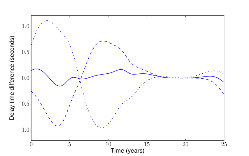
Figure 1: The difference in the planet-induced light-travel-time (LTT) delays of Keplerian versus Newtonian models for a typical two-planet fit for NN Ser. Three cases are shown: astrocentric (dashed-dotted), Jacobi (dashed) and modified Jacobi (solid). The $\mathrm{MJD}=54500$ reference time corresponds to the time around 19 years in when all models agree. For reference the LTT variations in NN Ser have a range of $\pm 40\,$seconds. The Newtonian comparison orbits are calculated separately for each of the three coordinate systems.

compares the difference between Keplerian and Newtonian predictions for the three parameterisations for an orbit typical of NN Ser. The ordering seen here with astrocentric coordinates worst, and our modified version of Jacobi coordinates best, agrees with what we found looking at a much broader range of orbit fits. The differences in Fig. 1 range from a few tenths of a second to more than one second, which given the timing precision of NN Ser can be expected to have a noticeable effect upon parameters. There are instances where deviations as large as 5 seconds occur, typically on dynamically very unstable orbits. We will see that these can have a quantitative effect upon the parameters, meaning that Keplerian models, whatever the coordinate parameterisation, are not adequate for fitting the NN Ser times. In consequence, the majority of the orbit fits in this paper, were undertaken using Newtonian $N$-body integrations, without Keplerian approximation. We employed the modified Jacobi representation to translate from orbital elements to initial position and velocity vectors to initialise these integrations, because, as Fig. 1 shows, they are the best of the three we investigated. We make one exception where we compare the results from $N$-body integrated and equivalent Keplerian models, based in each case upon the modified Jacobi prescription. When we need to specify exactly what system we are using, we will use expressions such as “astrocentric Keplerian” and “Newtonian modified Jacobi”. The first means orbits in which two astrocentric vectors execute Kepler ellipses, i.e. an approximation; the second means that Jacobi coordinates are used to initialise the orbits, using our modified version of angular frequency, but thereafter the paths are computed using $N$-body integration with no approximation beyond numerical uncertainties.

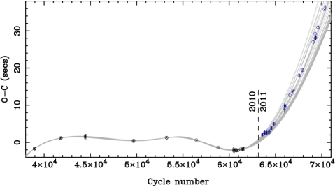
Figure 2: Eleven years of eclipse times of NN Ser, starting in May 2002. The dashed line marks the end of 2010; the data before this point are those listed in Beuermann et al. (2010), including the two updates listed in Table 1. The times are plotted relative to the ephemeris $\mathrm{BMJD(TDB)}=47344.0258547+0.1300801135E$, where $E$ is the cycle number. This was chosen to give a flat trend in times from 2002 to 2010. The light-grey smooth curves show 50 Newtonian orbit fits to the pre-2011 data only, generated via MCMC iteration, corresponding to the models of the lower-left panel of Fig. 4; the models were picked from the final 100 models of the MCMC chain. The times after 2010 are from this paper and were not used to create the fits, and yet they match the predicted trend well. For clarity, only data with uncertainties $<2\,$sec are shown.

3.2 Model fitting approach

Sometimes-sparse coverage, and often-long orbital periods, mean that timing work on circum-binary planets is plagued by degeneracies amongst fit parameters. This can cause problems simply in locating best-fit models, and even more so in the determination of uncertainties. For instance the widely-used Levenberg-Marquardt method often fails to locate the minimum in such circumstances and the covariance matrix it generates can be far from capturing the complexity of very non-quadratic, and possibly multiple minima. A widely-used method that can overcome these difficulties, which we adopt here, is the Markov Chain Monte Carlo (MCMC) method. The aim of MCMC analysis is to obtain a set of possible models distributed over model parameter space with the Bayesian posterior probability distribution defined by the data. This is accomplished by stochastic jumping of the model parameters, followed by selection or rejection according to the posterior probability of the model $M$ given the data $D$, $P(M|D)$. This process results in long chains of models, which, if long enough to be well-mixed, have the desired probability distribution. By Bayes’ theorem the posterior probability is proportional to the product of the prior probability of the model, $P(M)$, and the likelihood, $P(D|M)$, which in our case is determined by the factor $\exp(-\chi^{2}/2)$, where $\chi^{2}$ is the standard goodness-of-fit parameter.

For the prior probabilities, we adopted uniform priors for all temporal zero-points, the eccentricities (0 to 1), and the arguments of periapsis ($-180^{\circ}$ to $+180^{\circ}$). We used Jeffreys priors ($1/a$, $1/m$) for the semi-major axes and masses. Some care is needed over the eccentricity $e$ and the argument of periapsis $\omega$, which sets the orientation of the ellipse in its own plane, because $\omega$ becomes poorly constrained as $e\rightarrow 0$. This can cause difficulties if one iterates using $e$ and $\omega$ directly. We therefore transformed to $x=\sqrt{e}\cos\omega$ and $y=\sqrt{e}\sin\omega$, which since the Jacobian $||\partial(x,y)/\partial(e,\omega)||$ is constant, maintains uniform priors in $e$ and $\omega$, but causes no difficulties for small values of $e$. The choice of priors has a small but non-negligible effect upon the results. For instance we find a significant range of semi-major axes in some models, and there is clearly a difference between a uniform prior and $1/a$. Although the priors can have a quantitative effect upon results in such cases, they have no qualitative impact upon the conclusions of this paper.

Armed with the MCMC runs, we are in a position to compute uncertainties, and correlations between parameters. The MCMC method is useful in cases of high dimensionality such as we face here (the models we present require from 10 to 13 fit parameters) and can give a good feel for the regions of parameter space supported by the data. Requiring no derivative information, it is highly robust, a significant point for the Newtonian models where one can generate trial orbits which do not even last the span of the observed data. These cause difficulties for derivative-based methods such as Levenburg-Marquardt for example. Generation of models with the correct posterior probability distribution is also ideal for subsequent dynamical analysis where one wants to tests models that are consistent with the data.

The main disadvantage of the MCMC method is the sometimes-large computation time needed to achieve well-mixed and converged chains. The way in which the models are jumped during the iterations is important. Small jumps lead to slow random-walk behaviour with long correlation times, while large jumps lead to a high chance of rejection for proposed models and long correlation times once more. Ideally one jumps with a distribution that reflects the correlations between parameters, but it is not always easy to work out how to do this, and there is no magic bullet to solve this in all cases. For instance if multiple minima are separated by high enough $\chi^{2}$ “mountains”, a chain may never jump between them. In this paper we adopted the affine-invariant method implemented in the Python package emcee (Foreman-Mackey et al., 2013). This adapts its jumps to the developing distribution of models, which is a great advantage over having to estimate this at the start, but even so, the problem in this case turned out to be one of the most difficult we have encountered, and in several cases we required $>10^{9}$ orbits to reach near-ergodic behaviour. We computed the autocorrelation functions of parameters as one means of assessing convergence, but our main method, and the one we trust above any other, was visual, by making plots of the mean and root-mean-square (RMS) values of parameters as a function of update cycle number along the chains. Initial “burn-in” sections are obvious on such plots, as are long-term trends. There is no way to be absolutely certain that convergence has been reached in MCMC because there can be regions of parameter space that barely mix with each other. Even if one computed $10^{10}$ models, there would be no guarantee that a new region of viable models would not show up after $10^{12}$. From the very many computations we have carried out, including large numbers of false starts, we believe that we have explored parameter space very fully, and there are no undiscovered continents of lower $\chi^{2}$. However, as we will describe later, we did encounter one case that converged too slowly to give reliable results. This is fundamentally an issue of degeneracy and it should improve greatly with further coverage.

3.3 Predicting the future

We start our analysis with our primary objective: how well does the two-planet model developed by Beuermann et al. (2010) fare when confronted with new data? Fig. 2 shows the most recent eleven years of data on NN Ser, dating back to May 2002 when we first started to monitor it with ULTRACAM. The vertical dashed line at the end of 2010 marks the boundary between the times listed in Beuermann et al. (2010) and the new times of this paper. The grey curves are a sub-set of 50 MCMC-generated Newtonian models based upon Beuermann et al. (2010)’s times alone. Without the new times or orbit fits to guide the eye, one might have guessed that the new times would perhaps range in $O-C$ around $\pm 3\,\sec$ on this plot. However earlier data, which are included in the fits, but off the left-hand side of the plot windows (see Beuermann et al. (2010) and Fig. 9 later in this paper), cause the planet model to predict a sharp upturn since 2010, corresponding to delayed eclipse times as the binary moves away from us relative to its mean motion during the previous 8 years. In the planetary model, the upturn is primarily the result of the $7\,\mathrm{M}_{\mathrm{J}}$ outermost planet. Our new data are in remarkably good agreement with this (remarkable to the authors at least). While this is not a proof of the planetary model, it has nevertheless passed the test well. We can’t say for sure that alternative models such as those of Applegate (1992) don’t have a similarly precise “memory” of the past, but neither is it clear that they do, whereas it is a key prediction of the clockwork precision of Newtonian dynamics.

Including the new times when generating the fits, gives a much tighter set of possible orbits illustrated in Fig. 3

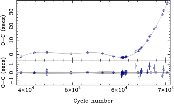
Figure 3: This plot is identical to Fig. 2 but now the orbital fits are based upon all data, incorporating the new times, and it includes a plot of the residuals relative to the best of the orbits shown. For clarity, only points with uncertainties $<0.5\,$sec are shown.

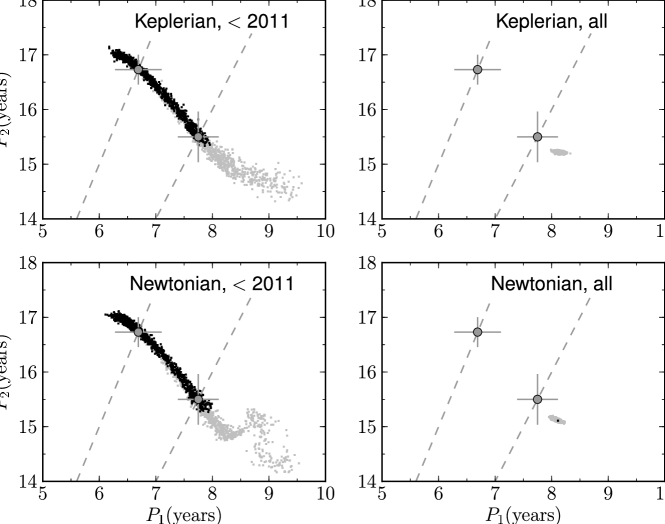
Figure 4: Regions of $P_{1}$–$P_{2}$ space supported by the data, shown in each case using 2000 models sampled from MCMC chains. The top-left panel is our equivalent of Beuermann et al. (2010), i.e. we use only data taken before 2011 and assume Keplerian orbits (although our Jacobi formalism leads to a very small change in position). The top-right panel shows Keplerian models based upon all of the data; the lower panels show the corresponding results for Newtonian orbit integrations. The grey dashed lines mark 2:1 (right-hand) and 5:2 (left-hand) period ratios, while the crosses mark the models “2a” (lower right) and “2b” (upper left) from Beuermann et al. (2010). Black (grey) points delineate models which last either more (less) than 1 million years, the post-common-envelope age of NN Ser.

which also shows residuals between the data and the best of the fits shown. It should be noted however that at this point we are following Beuermann et al. (2010)’s assumption of zero eccentricity for the outer orbit, which is largely responsible for the very tightly defined fit. The dispersion increases once this constraint is lifted (independent of whether Newtonian or Keplerian models are adopted).

3.4 Comparison with Beuermann et al. (2010)

The fits plotted in Figs 2 and 3 were based upon allowing the same parameters to vary as used in Beuermann et al. (2010)’s model ”2a” (their best one), so in this section we look at the effect that the new data has upon the parameters. We also consider the difference made by using integrated Newtonian models compared to Keplerian orbits; in all subsequent sections we use Newtonian models only. For reference, in their (astrocentric Keplerian) model 2a, Beuermann et al. (2010) allowed a total of 10 parameters to be free which were the zero-point and period of the binary’s ephemeris, the period, semi-major axis and reference epoch of the outer planet, and the period, semi-major axis, reference epoch, eccentricity and argument of periastron of inner and lower mass planet. The orbit of the outer planet was assumed to be circular.

Beuermann et al. (2010) give a detailed description of their fits in terms of the periods “$P_{c}$” and “$P_{d}$” of the two planets (corresponding to our $P_{2}$ and $P_{1}$), so we first focus upon this. Fig. 4 shows the range of $P_{1}$–$P_{2}$ space supported under either the Keplerian or Newtonian interpretations, and making use of either the data used by Beuermann et al. (2010) only, or the full set including our new times. The top-left panel is equivalent to Beuermann et al. (2010) and indeed matches the range of models they located, although the MCMC results show that the supported region is more complex than their division into just two models perhaps suggests. The top-right panel shows a significant shrinkage with the addition of new data and supports Beuermann et al. (2010)’s selection of their model 2a. While some shrinkage is expected, the extent of the change is notable, given that we have have only increased the baseline of coverage by around 15%. We believe this is a combination of degeneracy when fitting to pre-2011 data alone, combined with our having turned the corner of another orbit of the outer planet (planet 2), as shown by Fig. 2. Beuermann et al. (2010) found that there is little to choose between their two models in terms of goodness of fit, although their model 2a was marginally favoured. This is confirmed by the stripe of viable models connecting their 2a and 2b in the top-left panel of Fig. 4.

The lower panels show that, even though our choice of coordinates was motivated by the desire to generate Keplerian orbits which matched Newtonian orbits as closely as possible, there are nonetheless regions of parameter space considerably affected by three-body effects. In particular, the kink in the lower-left panel located in the region where the period ratio is closer than 2:1, compared to its relatively simple Keplerian counterpart in the upper-left panel, is evidence of this. Here deviations between Keplerian and Newtonian orbits amount to several seconds, highly significant given the precision of the NN Ser times, and the favoured parameter distribution is distorted as a result. The effects are much smaller above the 2:1 line, and show that the modified Jacobi coordinates can work well. Strangely enough, as we remarked earlier, although three-body effects are significant, the data are not good enough to prove that they operate (which could provide compelling independent support for the planet model) because there is sufficient degeneracy for either Keplerian or Newtonian models to fit the data equally well, albeit with differing sets of orbital elements. Obviously, if there are planets orbiting the binary in NN Ser, the weight of 300 years of classical mechanics favours Newtonian models, but it will be some time before this can be proved from the data directly.

3.5 Dynamical stability

As discussed earlier, some proposed circum-binary orbits have been shown to be unstable on short timescales, and if multiple planetary orbits are proposed, a check on their stability is essential. Having said this, all the data needed for this are not to hand since we don’t know the mutual orientations of the planets’ orbits. Therefore, in the absence of evidence to the contrary, we assume, along with previous researchers, that the orbits are coplanar. In addition we assume that, like the binary itself, we see the planetary orbits edge-on and for simplicity we set the orbital inclinations precisely to $90^{\circ}$. This minimises the masses of the planets relative to the binary, which will usually tend to promote stability. NN Ser emerged from its common envelope phase around one million years ago, and prior to this phase would have been significantly different, so we checked for stability by integrating backwards in time for just 2 million years. To a certain extent stability is already included within the Newtonian MCMC runs (lower panels of Fig. 4) since some proposed orbits generated by MCMC jumps lead to collisions within the span of the data and are rejected. It would have been easy to extend this so that all long-term unstable orbits were similarly thrown out, however, the CPU time penalty is far too great to allow this approach. Instead, our approach during the MCMC runs was simply to integrate for the 25 year baseline of the observations, leaving the longer-term dynamical stability computations to the small fraction of models retained (of order 1 in $10^{4}$) as we waited for the MCMC chains to reach a stable state.

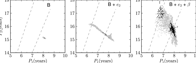
Figure 5: Regions of $P_{1}$–$P_{2}$ space supported by the data, showing the change as the models are given greater freedom. The left-most panel is the constrained model 2 (“B” for short) from Beuermann et al. (2010) for reference (i.e. it is identical to the lower-right panel of Fig. 4). In the centre panel, the eccentricity of the outermost planet is allowed to be non-zero, while the right-most panel allows the binary’s period to change in addition. Each panel shows 2000 Newtonian models based upon all of the data. As before, the grey dashed lines mark 2:1 (top) and 5:2 (bottom) period ratios, and black and grey points indicate stable and unstable models. From left-to-right, 0.02%, 0.7% and 15% of the models last more than 1 million years.

The differently shaded symbols in Fig. 4 distinguish between “stable” orbits which last for $>1$ million years (black) from the “unstable” ones which do not (grey). In the upper-left panel, orbits are mostly unstable below the 2:1 line (i.e. less extreme ratio), as one might expect. They are stabilised near the 2:1 and 5:2 lines and there is a mixed set of unstable and stable models in between. The pattern of stability and instability is broadly consistent with Beuermann et al. (2010)’s results, although our models seem to be more stable between the 2:1 and 5:2 lines than their description suggests. The topology of stable and unstable regions survives the distorting influence of Newtonian effects in the lower-left panel. Of order 50% of these models proved to be stable. Once the new data are included (right-hand panels), the supported models are confined to the largely unstable region lying below the 2:1 line in Fig. 4. Unsurprisingly therefore, very few of these models turn out to be stable – around 1 in 6000. Although one could argue that just one stable model consistent with the data is all that is required to claim potential stability, the reduction in the fraction of stable models is a worry for the planet model of NN Ser, because it looks possible that with yet more data, we are likely to be left with no long-lived models at all. Thus we now turn to look at the consequences of freeing up the orbit fits by allowing non-zero eccentricity in the outermost planetary orbit and changes in the orbital period of the binary itself.

3.6 Eccentricity and binary orbital period variation

We have so far followed Beuermann et al. (2010)’s application of Ockham’s razor by choosing the most restrictive model consistent with the data. This helps the fitting process because of degeneracies, as Beuermann et al. (2010) suggest, but it gives an overly optimistic view of how well constrained NN Ser is. In following Beuermann et al. (2010)’s model 2, we are making the questionable assumptions that the outer planet has a circular orbit and that NN Ser acts as a perfect clock. While we don’t need to deviate from these in order to find good fits to the data, it would come as little surprise if they were not entirely accurate, so it is of interest to examine the effect relaxing these restrictions has upon the model parameters, and also upon the issue of stability, which, as we have just seen, is looking marginal in the light of the new data. We therefore carried out MCMC runs with the outermost planet’s orbit allowed to be eccentric (two extra free parameters, making 12), and then with the addition of “clock drift” in the form of a quadratic term $\beta$ in the binary ephemeris, bringing the number of free parameters to 13. We found that the MCMC chain of the last case never converged owing to a strong degeneracy between the quadratic term and the orbit of the outer planet which allowed $a_{2}$ to range up to values $>12\,$AU compared to a value $\approx 5.4\,$AU when no quadratic term was included. In order to force convergence upon a reasonable timescale, we therefore applied a gaussian prior on $\beta$, where the latter is defined by its appearance in the ephemeris relation

$$T=T_{0}+PE+\beta E^{2},$$ (17)

with $E$ the eclipse cycle number and $T$ the time in days. The prior we applied was $P(\beta)\propto\exp(-(\beta/\sigma_{\beta})^{2}/2)$, with $\sigma_{\beta}=7.5\times 10^{-14}\,$days, 25 times the magnitude expected for gravitational wave losses (see later). This allows significant extra freedom, without suffering the convergence issues of the unconstrained model. The constraint on $\beta$ allows the majority of the values we found when there was no constraint at all, but cuts off an extended wing that reaches values as high as $\beta=1.5\times 10^{-12}\,$days.

Fig. 5 shows the change in the $P_{1}$–$P_{2}$ MCMC projection as the orbital models are given these greater freedoms. The changes are large, showing that parameter degeneracy remains significant. The orbital parameters are consequently much more uncertain than the constrained model 2 of Beuermann et al. (2010) suggests, and it is no longer even clear whether their model 2a (near 2:1) is favoured over 2b (5:2) as we see islands of stability corresponding to both solutions. Perhaps most importantly however, the increased model freedom allows access to long-lived parts of parameter space, with significant regions of stability, somewhat allaying the worry of the previous section over the likely complete disappearance of any such models. This is particularly the case once the binary’s period is allowed to vary.

The means and standard deviations of the orbital parameters of models plotted in Fig. 5 are listed in Table 2, along with the

Table 2: The first three columns list the means and standard deviations of the orbital parameters of the models shown in Fig. 5. The model of the left-hand column uses the same fit parameters as Beuermann et al. (2010)’s model 2, hence the “B”, with the next two adding the extra freedoms indicated. The right-hand column is the same as the left-hand one except only the pre-2011 data were used. The reference eclipse for the binary ephemeris, marked by $T_{0}$, is shifted forward by 43042 cycles relative to the usual ephemeris of NN Ser to reduce the otherwise-strong correlation between $T_{0}$ and $P$.

Parameter	B	B + $e_{2}$	B + $e_{2}$ + $\beta$	B
	all	all	all	pre-2011
$T_{0}-52942.9338$ (MJD)	$(9.5\pm 0.1)\times 10^{-5}$	$(8.4\pm 2.8)\times 10^{-5}$	$(5.3\pm 4.4)\times 10^{-5}$	$(9.2\pm 0.8)\times 10^{-5}$
$P-0.13008014$ (d)	$(2.4\pm 0.1)\times 10^{-9}$	$(2.3\pm 0.3)\times 10^{-9}$	$(2.7\pm 0.5)\times 10^{-9}$	$(1.8\pm 2.6)\times 10^{-9}$
$\beta$ ($10^{-12}\,\mathrm{d}$)	—	—	$0.04\pm 0.05$	—
$a_{1}$ (AU)	$3.488\pm 0.012$	$3.43\pm 0.14$	$3.37\pm 0.15$	$3.28\pm 0.22$
$P_{1}$ (yr)	$8.09\pm 0.04$	$7.9\pm 0.5$	$7.7\pm 0.5$	$7.4\pm 0.8$
$m_{1}$ ($\mathrm{M}_{\mathrm{J}}$)	$2.688\pm 0.036$	$2.3\pm 0.5$	$2.2\pm 0.5$	$2.2\pm 0.9$
$T_{1}$ (MJD)	$58205\pm 22$	$58106\pm 228$	$58043\pm 250$	$57826\pm 378$
$e_{1}$	$0.163\pm 0.007$	$0.19\pm 0.05$	$0.19\pm 0.04$	$0.21\pm 0.04$
$\omega_{1}$ (∘)	$-107.4\pm 2.7$	$-111\pm 13$	$-118\pm 15$	$-105\pm 8$
$a_{2}$ (AU)	$5.313\pm 0.005$	$5.35\pm 0.06$	$5.47\pm 0.15$	$5.51\pm 0.18$
$P_{2}$ (yr)	$15.125\pm 0.021$	$15.27\pm 0.28$	$15.8\pm 0.7$	$16.0\pm 0.8$
$m_{2}$ ($\mathrm{M}_{\mathrm{J}}$)	$7.46\pm 0.05$	$7.33\pm 0.31$	$7.29\pm 0.32$	$6.9\pm 1.4$
$T_{2}$ (MJD)	$53973.3\pm 1.5$	$54016\pm 106$	$54096\pm 133$	$54008\pm 58$
$e_{2}$	—	$0.08\pm 0.05$	$0.09\pm 0.05$	—
$\omega_{2}$ (∘)	—	$43\pm 119$	$62\pm 95$	—
$\chi^{2}$, $N_{dof}$	62.8, 66	62.6, 64	62.5, 63	31.8, 32

values corresponding to the lower-left panel of Fig. 4. Most of the parameters have an obvious meaning, but it should be noted that the epochs $T_{1}$ and $T_{2}$ refer to the time when the respective planet reaches the ascending node of its orbit, not the more usual periastron, as the latter is poorly defined for small eccentricities. The eccentricity of the outer planet $e_{2}$ and the quadratic term in the binary ephemeris $\beta$ are consistent with zero, although, as we have just seen, dynamical stability seems to suggest that $e_{2}>0$, and it would not be surprising were this the case. The $\chi^{2}$ values listed are the minimum of any models of the MCMC chains. The MCMC method does not aspire to find the absolute minimum $\chi^{2}$, and tests we have made suggest that the values listed in the table are of order $0.5$ – $1.5$ above the absolute minimum. The improvement in $\chi^{2}$ as more parameters are added is marginal, so a circular outer orbit is fine for fitting the data. It is the requirement of dynamical stability which leads us to favour the model with eccentricity. In using the numbers of Table 2, it should be realised that the mean values do not need to correspond to any viable model: for instance, the mean of a spherical shell distribution lies outside the distribution itself.

The quadratic term produced by a rate of angular momentum change $\dot{J}$ is given by

$$\beta=\frac{3P^{2}}{2}\frac{\dot{J}}{J},$$ (18)

where $P$ is the orbital period and $J$ is the angular momentum. For the parameters of NN Ser (Parsons et al., 2010a), gravitational wave radiation alone gives $\dot{J}/J=-1.36\times 10^{-18}\,\sec^{-1}$, and therefore $\beta=-3.0\times 10^{-15}\,$days. Over the entire baseline of observations of NN Ser, the $\beta E^{2}$ term would then amount to $1.5\,\sec$. Although in principle this is detectable, at present, because of the planets (or whatever is causing the timing variability), there is strong degeneracy in the fits once a quadratic term is allowed and we are far from being able to measure a term this small. In fact, as we remarked earlier, the degeneracy between $\beta$ and the outermost planet’s orbital parameters is so strong that $\beta$ is only weakly constrained by our data and the uncertainty listed for $\beta$ in Table 2 largely reflects the prior restriction we placed upon it. The GWR prediction is the minimum expected angular momentum loss, as one also expects some loss from magnetic stellar wind braking. The secondary star in NN Ser has a mass of $0.111\,\mathrm{M}_{\odot}$, making it comparable to short-period ($P\approx 90\,$mins) cataclysmic variables for which there is evidence for angular momentum loss at around $2.5\times$ the GWR rate at the same short periods (Knigge et al., 2011), but this is still much smaller than we can measure at present. We expect a substantial improvement in this constraint over the next few years as the parameter degeneracy is lifted. Given the current lack of constraint upon $\beta$ from the data, at present we favour the model in which $\beta$ is fixed to zero.

3.7 Comparison with Beuermann et al. (2013)

As mentioned earlier, shortly after the first submission of this paper, Beuermann et al. (2013) presented new eclipse times and a stability analysis of NN Ser. In this section we compare our sets of results which are based upon the same set of data prior to 2011, but independent sets of new data thereafter, i.e. we do not use any of their new data. Beuermann et al. (2013) consider only models equivalent to our “$B+e_{2}$” models of the middle panel of Fig. 5. They fitted their data through Levenberg-Marquardt minimisation of $\chi^{2}$, which, apart from the absence of prior probability factors, finds the region of highest posterior probability, but does not explore the shape of region of parameter space supported by the data as MCMC does. They imposed conditions of dynamical stability, which makes a direct comparison with our results tricky since we adopted the strategy of first seeing what parameter space was supported by the data and only then testing dynamical stability. They found stable orbits close to the 2:1 resonance if they allowed the orbit of the outermost planet to be eccentric. This is consistent with what we find: there are almost no long-lived orbits if the outermost orbit is forced to be circular, but some appear near the 2:1 line once eccentricity is allowed. We refer to Beuermann et al. (2013) for a detailed discussion of the nature of the stable solutions that they find, in particular a demonstration that they are in mean-motion resonance. Beuermann et al. (2013) did not consider any period variation of the binary or explore the much wider range of orbits this allows. Thus they did not uncover any of the stable models near the 5:2 ratio which are permitted by the data once period variation is included, and therefore, although we agree that the 2:1 resonance is favoured, we feel that their exclusion of the 5:2 resonance at “99.3% confidence” is premature.

Beuermann et al. (2013) present a plot of the dynamical lifetime as a function of the eccentricities of the two planets, $e_{1}$ and $e_{2}$ (their figure 3). This provides us with an opportunity to compare the constraints set by our two sets of data, although as already remarked the differences between our two approaches make exact comparison difficult. For instance, we reject the implication of the right-hand two panels of their figure 3 that the dynamical lifetime is a single-valued function of $e_{1}$ and $e_{2}$; instead, once one allows for the distribution of other parameters, there must be a distribution of lifetimes at any given values of $e_{1}$ and $e_{2}$; we discuss a similar issue at length in the next section. However, a comparison can still be made accepting that Beuermann et al. (2013)’s figure shows the lifetime of the most probable orbits, since for each $e_{1}$–$e_{2}$ point they re-optimised the other 10 parameters. Our nearest equivalent to their plot is shown in Fig. 6

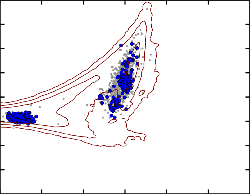
Figure 6: The projection onto the $e_{2}$–$e_{1}$ plane of the MCMC chain allowing for eccentricity in both orbits but not binary period change, i.e. the models shown in the central panel of Fig. 5. The contours show regions encompassing $68.3$, $95.4$ and $99.7$% of the orbits supported by the data, with no restriction on stability. Small grey dots mark the orbits that last between $10^{6}$ and $50\times 10^{6}$ years; large blue dots mark those that last for more than $50\times 10^{6}$ years. The contours are comparable to the left panel of figure 3 from Beuermann et al. (2013), while the locations of the long-lived models are comparable to the other two panels of their figure.

for which we extended our dynamical integrations to 100 million years to delineate regions of greatest long-term stability. The figure compares well with figure 3 of Beuermann et al. (2013) with many similar features. We see the same tight definition of $e_{1}$ at low values of $e_{2}$, but spreading out as $e_{2}$ increases. The main island of stable models found by Beuermann et al. (2013) coincides with the island of stable orbits that have high $e_{2}$ values seen in Fig. 6.

There are a few differences as well. Our data support a smaller region of parameter space, owing to a higher overall precision which more than compensates for a smaller number of eclipse time measurements. In particular, a spur of large $e_{2}$ / low $e_{1}$ allowed by Beuermann et al. (2013)’s data is eliminated by ours, and there is general exclusion of high $e_{2}$ values leading to the large area of white space on the right-hand side of the plot for which we chose the same axis limits as Beuermann et al. (2013). We ascribe these differences to signal-to-noise rather than anything more fundamental. The other most notable difference is that we find an island of stability for $e_{2}=0.01$ – $0.04$ as well. Although there are signs of the same region in Beuermann et al. (2013)’s figure, it is not as marked as we find. This may be the result of the difference in approaches, with Beuermann et al. (2013) tracing the highest probability region for each $e_{1}$–$e_{2}$ value, versus our exploration of the larger region of supported parameter space.

These differences are small, and overall we conclude that we are in substantial agreement with Beuermann et al. (2013). This is of course to be hoped for given that we use the same data, with two small corrections, up to 2011.

4 Discussion

The two-planet model for the variations in eclipse times of NN Ser has survived both new precise data and an updated dynamical stability analysis. It is the first compact eclipsing binary apparently hosting planets for which this can be said. It also delivers by far the highest quality eclipse times with a weighted RMS scatter around the best fit orbit of $\sigma=0.07\,$sec, where

$$\sigma^{2}=\frac{\chi^{2}/(N-V)}{\left(\sum_{i=1}^{N}1/\sigma_{i}^{2}\right)/N},$$ (19)

with $N$ the number of data, $V$ the number of variable parameters, and $\sigma_{i}$ the individual uncertainties on the eclipse times. The nearest rival in this respect as far as we can determine is HU Aqr for which Goździewski et al. (2012) quote a scatter of $0.7\,$sec, and this after significant pruning of discrepant points. Our typical best-fit values of $\chi^{2}$ are around 63 with 76 points and 10 – 13 fit parameters. The expected value of $\chi^{2}$ is thus 63 to 66 $\pm 11$, so there are as yet no signs of systematics in the data.

We have shown that the range of orbits consistent with Beuermann et al. (2010)’s data leads to a good prediction for the location in the $O-C$ diagram of the new data, so the planet model has predictive power. Moreover, allowing a non-zero eccentricity of the outer planet’s orbit, we find stable solutions. The latter result is interesting, and perhaps counter-intuitive at first sight. One might expect if the outer planet’s orbit is allowed to be eccentric then it is more likely to de-stabilise the orbit of the lighter inner planet. This is what Horner et al. (2012b) found, but we believe their analysis to suffer from significant technical flaws. Some of these are common to other papers from the same authors, as we now discuss.

4.1 Previous dynamical stability analyses of NN Ser and related systems

Beuermann et al. (2010) carried out a limited stability analysis of NN Ser’s putative planetary system using $100$,$000\,\mathrm{yr}$-long integrations and identified stable regions of parameter space, which they tentatively associated with 2:1 and 5:2 mean-motion resonances. Horner et al. (2012b) pointed out that $10^{5}\,\mathrm{yr}$ was too short to assess long-term stability, and also criticised the restriction to circular orbits for the outer planet. They too found significant stability when the outer planet was held in a circular orbit, but when they allowed its eccentricity to vary and re-fitted the orbits, they found that the solution lay within a broad region of very short-lived orbits, although uncertainties were sufficient to allow for some long lasting ones too. They concluded this from an examination of the lifetime of the system as a function of the inner-planet’s semi-major axis $a_{1}$ and eccentricity $e_{1}$ (their figure 5), and ascribed it to the significant eccentricity ($e_{2}=0.22$) they found for the outer planet’s orbit. Our results do not agree with theirs, and this is not simply to do with the new data, because we still find significant numbers of stable solutions when we restrict our analysis to the pre-2011 data used by Beuermann et al. (2010) and Horner et al. (2012b).

Instead, we believe that the work presented in Horner et al. (2012b) suffers from a series of flaws, the last of which renders it largely irrelevant to the question of stability of NN Ser. The same problem affects a series of similar papers from the same authors, and thus we devote this section to where we think this work has gone awry.

We start with minor issues. First of all, NN Ser is not, and never has been, a cataclysmic variable, and, since its white dwarf is hot ($T_{eff}\approx 60$,$000\,$K, Wood & Marsh (1991)), it only emerged from its common envelope around one million years ago. This renders most of Horner et al.’s 100 million year-long integrations superfluous since the system was undoubtedly very different prior to the common envelope in a way that cannot be modelled with the Newtonian dynamics of a few, constant point masses. Still, this does not alter Horner et al.’s claim of instability since they place NN Ser within a zone where orbits typically survive only $\sim 3000$ years. Another minor issue is that they used a total mass for NN Ser of $0.69\,\mathrm{M}_{\odot}$ from Haefner et al. (2004) rather than the more recent determination of $0.646\,\mathrm{M}_{\odot}$ from Parsons et al. (2010a) which was used by Beuermann et al. (2010), thus they were not self-consistent since they started from Beuermann et al. (2010)’s solutions. Once more however, this probably does not affect their essential claims. Their use of astrocentric Keplerian fits, both from Beuermann et al. (2010) and of their own devising, are further drawbacks, because, as discussed earlier, no Keplerian model is accurate enough to match the precision of the NN Ser times, and astrocentric coordinates perform worst of the three coordinate parameterisations we examined. However, our calculations indicate that this should not have made a qualitative difference to Horner et al.’s work either.

This brings us to what we believe is the major problem with Horner et al. (2012b)’s analysis, a problem which applies equally to the series of papers from the same group analysing stability in related systems. The figures upon which Horner et al. (2012b) base their conclusions show cuts through parameter space in which dynamical lifetime is plotted as a function of two orbital parameters perturbed by $\pm 3\sigma$ in a grid around their best-fit values, variously the semi-major axis, eccentricity and argument of periastron of the inner planet. The problem with all of them is that they do not represent orbits consistent with the data because in each case the remaining 10 free parameters have not been adjusted. Correlations between orbital parameters are highly significant. Rather than slices through parameter space which very rapidly fall out of the region supported by the data, what should be plotted are the lifetimes of the projection of models consistent with the data. In general, as we indicated earlier when discussing Fig. 6, the result is not even a single-valued function of position in a 2D projection, and it is quite possible to have very short- and very long-lived models right on top of each other, an impossibility in Horner et al. (2012b)’s presentation. The MCMC method delivers just what is needed through its generation of models which follow the posterior probability distribution implied by the data. Fig. 7

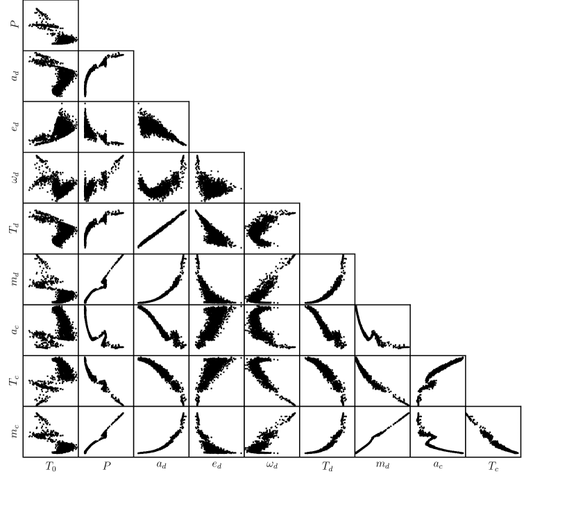
Figure 7: Scatter plots of the 10 parameters used during the MCMC runs shown in the lower-left panel of Fig. 4. These are based upon the pre-2011 data alone, with the outer planet held in a circular orbit and $N$-body effects accounted for.

displays all possible two-parameter projections of our MCMC models of the pre-2011 data and shows complex and high-degree correlations between all parameters. If anything, this figure undersells the problem since projections from high- to low-dimensionality smear out correlations (imagine projecting a spherical shell distribution from 3D to 2D for instance). Failing to account for these correlations is a serious error of methodology, and we believe it is this which explains the difference between our results and those of Horner et al. (2012b); Fig. 7 also makes it clear that covariance matrix uncertainties based upon a quadratic approximation to the minimum $\chi^{2}$ can under some circumstances be extremely mis-leading.

Fig. 8

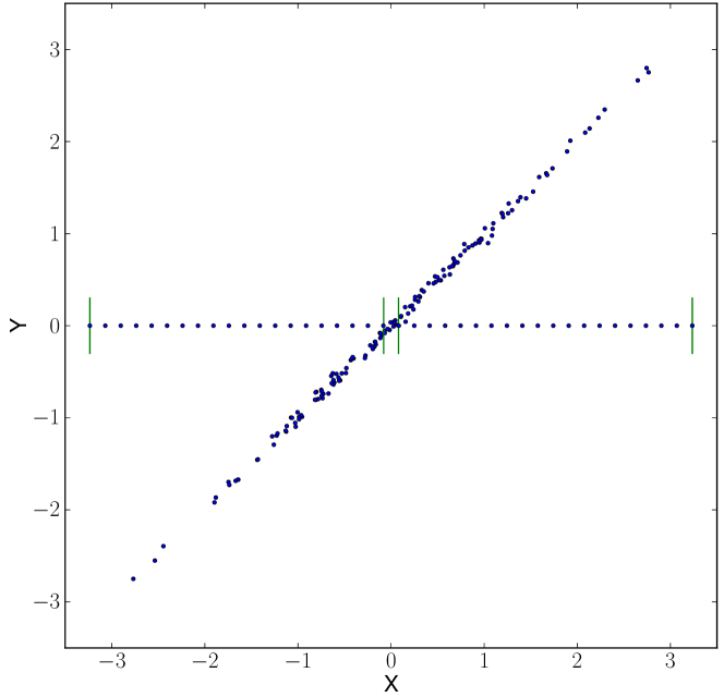
Figure 8: A schematic illustration of a serious problem with Horner et al. (2012b)’s stability analyses. The outermost vertical lines mark the $\pm 3\sigma$ range in $X$ of the correlated set of points. This range is much larger than the range covering the intersection of these points with the $X$-axis, as indicated by the innermost pair of vertical lines. The regularly-spaced points along the $X$-axis which span the $\pm 3\sigma$ range largely fall outside the region of the correlated points. The equivalents in Horner et al. (2012b) are the 2D grids over which they compute dynamical lifetimes; in the main these grids represent orbits which are incompatible with the data.

presents a schematic illustration of the problem with Horner et al. (2012b)’s approach. It compares $\pm 3\sigma$ range in $X$ of a set of points correlated in $X$ and $Y$ with the much smaller zone where these points intersect the $X$ axis. Under this analogy, Horner et al. (2012b)’s method is the equivalent of choosing a set of models that run along the $X$-axis over the $\pm 3\sigma$ range, as we show with the regularly-spaced points in Fig. 8. These barely sample the region of the correlated points; the problem can be expected to worsen with more dimensions. To assess the scale of the problem in the specific case of NN Ser, we calculated the size of the 2D intersection in a plot analogous to Horner et al. (2012b)’s figure 5 which covers $\pm 3\sigma$ ranges on the inner planet’s semi-major axis and eccentricity, $a_{1}$ and $e_{1}$. When just these two parameters are perturbed, we find that the $\chi^{2}$ minimum is nearly quadratic. We thus defined the intersection as the region for which $\chi^{2}-\chi^{2}_{\mathrm{min}}<13.8$ ($99.9$% two parameter, joint-confidence). We found that the interaction cross-section occupies just 1 part in $10^{4}$ of the total area plotted. In other words $99.99$% of the area plotted by Horner et al. (2012b) in their figure 5 is outside the region of 10-dimensional parameter space supported by the data, just as the regularly-spaced points in Fig. 8 are by-and-large outside the 2D distribution of points.

The problem with Horner et al. (2012b)’s analysis of NN Ser is of wide impact since a very similar approach was applied to HU Aqr by Horner et al. (2011) and Wittenmyer et al. (2012), NSVS 14256825 by Wittenmyer et al. (2013), HW Vir by Horner et al. (2012a) and, most recently, to QS Vir by Horner et al. (2013). In some cases these authors have averaged the results over other parameters such as the mean anomaly and argument of periastron of the particular planet orbit they perturb, but, as far as we can determine, in no case do they allow for simultaneous variations of all other fit parameters as is essential (and simply averaging over other parameters fails to account for the weighting required to reflect the constraints of the data in any case). We conclude that the issue of stability or instability in these systems needs re-opening. It may well turn out that the conclusions of this series of papers, which have for the most part found that proposed multi-planet orbits around binaries are not dynamically viable, will remain unchanged (we think it highly likely that the orbits proposed for QS Vir are unstable for instance), but some work is now required to be sure that this is the case. This problem does not apply to the recent study of NN Ser by Beuermann et al. (2013) because although their lifetime versus $e_{1}$–$e_{2}$ plots are superficially similar to Horner et al. (2012b)’s plots, Beuermann et al.’s optimisation of the other parameters ensures that they stayed in regions of parameter space supported by the data.

4.2 The immediate future of NN Ser

Since we have shown that the expected period change of the binary is much less than our current measurement uncertainty, our favoured model for NN Ser is one in which we allow the outer planet’s orbit to be eccentric, but do not allow for any change in binary period, i.e. the middle set from Fig. 5. Using this set of models, Fig. 9

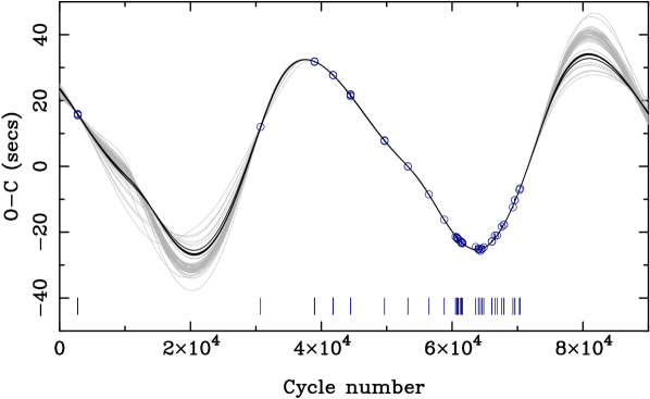
Figure 9: 50 orbit fits to NN Ser allowing for eccentricity in the outer planet’s orbit diverge in the near future. Darker lines highlight those models which are stable for more than a million years. The reference ephemeris for this plot is $\mathrm{BMJD(TDB)}=47344.0243673+0.130080141716E$. The plot extends until July 2020. Vertical lines at the bottom of the plot show the time sampling. Only points with uncertainties $<0.5\,$sec are shown.

shows all of the eclipse times of NN Ser with uncertainties less than 0.5 seconds, and projects a few years into the future. We are still paying the price for the poor coverage of the 1990s, but the next few years should see a great tightening of the constraints. It appears from this plot that a sampling interval of order a year or two should suffice.

4.3 The planet hypothesis of eclipse timing variations

Rather to our surprise, the new eclipse times of NN Ser presented in this paper are in good agreement with predictions based upon Beuermann et al. (2010)’s model in which two planets orbiting the binary cause the timing variations. We say to our surprise, because if all eclipse timing variations of compact binary stars are caused by planets, circum-binary planets must be common, since when looked at in detail the majority show timing variations (Zorotovic & Schreiber, 2013). We have long worried, and continue to worry, that the planet models are a glorified form of Fourier analysis, capable of fitting a large variety of smooth variations. We may simply have been lucky so far with NN Ser that the “orbits” returned have been stable, so, although our results are in line with the planet model, we do not regard the question as to the reality of the planets to be settled yet. Currently the main obstacle to a definitive answer is the still-considerable degeneracy in the orbit fits. Continued monitoring will cure this. However, it is notable that this degeneracy survives even with our mean timing precision of around $0.07\,$secs. Since one would need $\sim 200$ eclipse times of $1\,$sec precision to match a single time of $0.07\,$sec precision, we require not just extended coverage, but extended precision coverage. The ultimate goal should be to remove this degeneracy and, beyond this, detect $N$-body effects.

The planet model for NN Ser also survives the test of dynamical stability which has cut down so many other claims. Although we have challenged the methodology of many of these tests, we suspect that the general implication of implausibly unstable orbits found for many systems will prove to be correct. This is not the case for NN Ser yet, although it perhaps might be when further data are acquired, because the addition of new data has consistently made it harder to locate long-lived solutions. Around 50% of viable orbits fitted to the data of Beuermann et al. (2010) (with circular outer orbits) were long-lived. With our new data, this dropped to $0.02$%, prompting us to allow for eccentric outer orbits. Even allowing for eccentricity, we found a similar drop from $7.6$% to $0.7$% when we added the two ULTRACAM points from July 2013.

5 Conclusions

We have presented 25 new high precision eclipse times of the close white dwarf binary, NN Ser. The new times impressively follow the increasing delay predicted according to the two planet model presented by Beuermann et al. (2010). Moreover, some of the models supported by the full set of data are dynamically stable. We found during our analysis that the difference between Keplerian and properly integrated Newtonian models is significant compared to the data uncertainties and must be accounted for during fitting, not just in follow-up dynamical analysis.

The new data substantially reduce the degree of degeneracy in the planet model fits, but much still remains, especially if the models are given complete freedom with eccentricity in both orbits and orbital period change of the inner binary allowed. Such freedom may even be necessary as with the new data, very few of the orbits with the outer planet constrained to have a circular orbit are stable. With eccentricity allowed for both orbits we find orbital periods of $7.9\pm 0.5\,$yr and $15.3\pm 0.3\,$yr, and masses of $2.3\pm 0.5\,\mathrm{M}_{\mathrm{J}}$ and $7.3\pm 0.3\,\mathrm{M}_{\mathrm{J}}$, with stable orbits having close to 2:1 and 5:2 period ratios. At present, if a quadratic term is allowed in the binary ephemeris, degeneracy between it and the outermost planet’s orbit precludes an astrophysically significant measurement of the period change of the binary; this should improve significantly over the next few years.

Finally, we have demonstrated that several existing dynamical stability analyses of NN Ser and related systems are based upon a flawed methodology and require revision.

References

- Applegate (1992) Applegate, J. H., 1992, ApJ, 385, 621
- Beuermann et al. (2012) Beuermann, K., Dreizler, S., Hessman, F. V., Deller, J., 2012, A&A, 543, A138
- Beuermann et al. (2013) Beuermann, K., Dreizler, S., Hessman, F. V., 2013, A&A, 555, A133
- Beuermann et al. (2010) Beuermann, K., et al., 2010, A&A, 521, L60
- Beuermann et al. (2011) Beuermann, K., et al., 2011, A&A, 526, A53
- Brinkworth et al. (2006) Brinkworth, C. S., Marsh, T. R., Dhillon, V. S., Knigge, C., 2006, MNRAS, 365, 287
- Chambers (1999) Chambers, J. E., 1999, MNRAS, 304, 793
- Dai et al. (2010) Dai, Z.-B., Qian, S.-B., Fernández Lajús, E., Baume, G. L., 2010, MNRAS, 409, 1195
- Dhillon et al. (2007) Dhillon, V. S., et al., 2007, MNRAS, 378, 825
- Doyle et al. (2011) Doyle, L. R., et al., 2011, Science, 333, 1602
- Dvorak (1986) Dvorak, R., 1986, A&A, 167, 379
- Eastman et al. (2010) Eastman, J., Siverd, R., Gaudi, B. S., 2010, PASP, 122, 935
- Foreman-Mackey et al. (2013) Foreman-Mackey, D., Hogg, D. W., Lang, D., Goodman, J., 2013, PASP, 125, 306
- Gibson et al. (2008) Gibson, N. P., et al., 2008, A&A, 492, 603
- Goździewski et al. (2012) Goździewski, K., et al., 2012, MNRAS, 425, 930
- Haefner (1989) Haefner, R., 1989, A&A, 213, L15
- Haefner et al. (2004) Haefner, R., Fiedler, A., Butler, K., Barwig, H., 2004, A&A, 428, 181
- Hinse et al. (2012) Hinse, T. C., Lee, J. W., Goździewski, K., Haghighipour, N., Lee, C.-U., Scullion, E. M., 2012, MNRAS, 420, 3609
- Hobbs et al. (2006) Hobbs, G. B., Edwards, R. T., Manchester, R. N., 2006, MNRAS, 369, 655
- Horner et al. (2011) Horner, J., Marshall, J. P., Wittenmyer, R. A., Tinney, C. G., 2011, MNRAS, 416, L11
- Horner et al. (2012a) Horner, J., Hinse, T. C., Wittenmyer, R. A., Marshall, J. P., Tinney, C. G., 2012a, MNRAS, 427, 2812
- Horner et al. (2012b) Horner, J., Wittenmyer, R. A., Hinse, T. C., Tinney, C. G., 2012b, MNRAS, 425, 749
- Horner et al. (2013) Horner, J., Wittenmyer, R. A., Hinse, T. C., Marshall, J. P., Mustill, A. J., Tinney, C. G., 2013, ArXiv e-prints
- Kissler-Patig et al. (2008) Kissler-Patig, M., et al., 2008, A&A, 491, 941
- Knigge et al. (2011) Knigge, C., Baraffe, I., Patterson, J., 2011, ApJS, 194, 28
- Lee et al. (2009) Lee, J. W., Kim, S.-L., Kim, C.-H., Koch, R. H., Lee, C.-U., Kim, H.-I., Park, J.-H., 2009, AJ, 137, 3181
- Lee & Peale (2003) Lee, M. H., Peale, S. J., 2003, ApJ, 592, 1201
- Malhotra (1993) Malhotra, R., 1993, in Phillips, J. A., Thorsett, S. E., Kulkarni, S. R., eds., Planets Around Pulsars, vol. 36 of Astronomical Society of the Pacific Conference Series, p. 89
- Mustill et al. (2013) Mustill, A. J., Marshall, J. P., Villaver, E., Veras, D., Davis, P. J., Horner, J., Wittenmyer, R. A., 2013, ArXiv e-prints
- Parsons et al. (2010a) Parsons, S. G., Marsh, T. R., Copperwheat, C. M., Dhillon, V. S., Littlefair, S. P., Gänsicke, B. T., Hickman, R., 2010a, MNRAS, 402, 2591
- Parsons et al. (2010b) Parsons, S. G., et al., 2010b, MNRAS, 407, 2362
- Portegies Zwart (2013) Portegies Zwart, S., 2013, MNRAS, 429, L45
- Potter et al. (2011) Potter, S. B., et al., 2011, MNRAS, 416, 2202
- Press et al. (2002) Press, W. H., Teukolsky, S. A., Vetterling, W. T., Flannery, B. P., 2002, Numerical recipes in C++ : the art of scientific computing
- Qian et al. (2009a) Qian, S.-B., Dai, Z.-B., Liao, W.-P., Zhu, L.-Y., Liu, L., Zhao, E. G., 2009a, ApJLett., 706, L96
- Qian et al. (2010) Qian, S.-B., Liao, W.-P., Zhu, L.-Y., Dai, Z.-B., Liu, L., He, J.-J., Zhao, E.-G., Li, L.-J., 2010, MNRAS, 401, L34
- Qian et al. (2009b) Qian, S.-B., et al., 2009b, ApJLett., 695, L163
- Qian et al. (2011) Qian, S.-B., et al., 2011, MNRAS, 414, L16
- Steele et al. (2008) Steele, I. A., Bates, S. D., Gibson, N., Keenan, F., Meaburn, J., Mottram, C. J., Pollacco, D., Todd, I., 2008, in Society of Photo-Optical Instrumentation Engineers (SPIE) Conference Series, vol. 7014 of Society of Photo-Optical Instrumentation Engineers (SPIE) Conference Series
- Veras & Tout (2012) Veras, D., Tout, C. A., 2012, MNRAS, 422, 1648
- Welsh et al. (2012) Welsh, W. F., et al., 2012, Nature, 481, 475
- Wittenmyer et al. (2012) Wittenmyer, R. A., Horner, J., Marshall, J. P., Butters, O. W., Tinney, C. G., 2012, MNRAS, 419, 3258
- Wittenmyer et al. (2013) Wittenmyer, R. A., Horner, J., Marshall, J. P., 2013, MNRAS, 431, 2150
- Wood & Marsh (1991) Wood, J. H., Marsh, T. R., 1991, ApJ, 381, 551
- Zorotovic & Schreiber (2013) Zorotovic, M., Schreiber, M. R., 2013, A&A, 549, A95