Constraints on CP-violating Higgs couplings
to the third generation

Abstract

Discovering CP-violating effects in the Higgs sector would constitute an indisputable sign of physics beyond the Standard Model. We derive constraints on the CP-violating Higgs-boson couplings to top and bottom quarks as well as to tau leptons from low-energy bounds on electric dipole moments, resumming large logarithms when necessary. The present and future projections of the sensitivities and comparisons with the LHC constraints are provided. Non-trivial constraints are possible in the future, even if the Higgs boson only couples to the third-generation fermions.

1 Introduction

There is steady experimental progress in measuring the Higgs-boson couplings. Assuming for simplicity that deviations from the Standard Model (SM) manifest themselves predominantly in a single coupling, the couplings of the Higgs to $Z$ and $W$ bosons are known with an uncertainty of ${\mathcal{O}}(20-30\%)$, and to the third-generation fermions $t$, $b$, and $\tau$ with ${\mathcal{O}}(30\%)$, ${\mathcal{O}}(40\%)$, and ${\mathcal{O}}(60\%)$ relative errors, respectively (the sensitivity to the top-quark couplings arises from the loop processes $gg\to h$ and $h\to\gamma\gamma$) CMS-PAS-HIG-13-005 ; ATLAS-CONF-2013-034 ; Aad:2013wqa . The projected sensitivity for the 14 TeV LHC at 300 fb^-1 is ${\mathcal{O}}(4-15\%)$ and ${\mathcal{O}}(2-10\%)$ at 3000 fb^-1 of integrated luminosity Olsen:talk:Seattle . If deviations from the SM are found this would suggest that there is new physics (NP) close to the TeV scale. In this respect, CP-violating Higgs-boson couplings are particularly interesting, because any sign of CP violation in Higgs decays would constitute an indisputable NP signal.

Low-energy probes, such as electric dipole moments (EDMs), lead to severe constraints on CP-violating effects. The purpose of this paper is to derive the constraints that low-energy measurements set on CP-violating Higgs couplings to the third generation of fermions. In complete generality, we can write

$${\cal L}\supset-\frac{y_{f}}{\sqrt{2}}\left(\kappa_{f}\hskip 1.42262pt\bar{f}f+i\tilde{\kappa}_{f}\hskip 1.42262pt\bar{f}\gamma_{5}f\right)h\,,$$ (1)

where $f=t,b,\tau$ and $y_{f}=\sqrt{2}m_{f}/v$ is the SM Yukawa coupling with $m_{f}$ the fermion mass and $v\simeq 246\,{\rm GeV}$ the electroweak symmetry breaking vacuum expectation value of the Higgs field. The couplings $\tilde{\kappa}_{f}$ are CP violating, while $\kappa_{f}$ parametrize CP-conserving NP contributions. In the SM we have $\kappa_{f}=1$ and $\tilde{\kappa}_{f}=0$. Our primary aim is to derive bounds on the coefficient $\tilde{\kappa}_{f}$ using low-energy data. These can then be used as a useful target for direct searches at the LHC Berge:2008wi ; Berge:2008dr ; Berge:2011ij ; Fermilab:CPV ; Nishiwaki:2013cma ; Htt:CPV . Similarly, one could search for CP-violating Higgs-boson couplings to gauge bosons both at the LHC Godbole:2007cn ; Coleppa:2012eh ; Stolarski:2012ps ; Bolognesi:2012mm ; Boughezal:2012tz ; Chatrchyan:2012jja ; ATLAS:spin ; Freitas:2012kw or utilizing low-energy observables McKeen:2012av . Note that there could also be other contributions to the EDMs beyond the ones we discuss, for instance from complex flavor-violating couplings of the Higgs with the corresponding bounds given in McKeen:2012av ; Giudice:2008uua ; Goudelis:2011un ; Blankenburg:2012ex ; Harnik:2012pb .

The paper is organized as follows. Focusing first on the CP-violating Higgs-top couplings we deduce the corresponding constraints from EDMs in Sec. 2 and from the LHC Higgs data in Sec. 3. The combined effect of the two types of constraints as well as the projected future sensitivities are presented in Sec. 4. Analogous constraints on bottom and tau couplings to the Higgs are derived in Sec. 5. In Sec. 6 we summarize our main findings. A series of appendices completes our work. The details about the renormalization group (RG) analysis for the neutron EDM are given in App. A, while the RG resummation of the bottom-quark contributions to the neutron EDM is discussed in App. B. Finally, in App. C the constraints on the CP-violating couplings of the Higgs to third-generation fermions arising from flavor-changing neutral current processes are briefly examined.

2 Constraints from EDMs

EDMs are very sensitive probes of NP that contains new CP-violating weak phases. They can probe scales as high as $10^{8}\,{\rm GeV}$ Cirigliano:2013lpa ; Engel:2013lsa ; Pospelov:2005pr . Here we are interested in the constraints that the EDM measurements impose on the CP-violating Higgs-top coupling, i.e. the coefficient $\tilde{\kappa}_{t}$ in Eq. (1). The derivation of constraints on the Higgs-boson couplings to bottom quarks and tau leptons is relegated to Sec. 5.

2.1 EDM of the electron

The CP-violating Higgs-boson coupling to the top quark induces an electron EDM

$${\cal L}_{\rm eff}=-d_{e}\,\frac{i}{2}\,\bar{e}\hskip 1.42262pt\sigma^{\mu\nu}\gamma_{5}\hskip 0.7113pte\,F_{\mu\nu}\,,$$ (2)

through a Barr-Zee type two-loop diagram, cf. Fig. 1 (left). The diagram with the photon propagator gives Barr:1990vd

$$\frac{d_{e}}{e}=\frac{16}{3}\frac{\alpha}{(4\pi)^{3}}\hskip 0.7113pt\sqrt{2}G_{F}\hskip 0.7113ptm_{e}\,\Big{[}\kappa_{e}\tilde{\kappa}_{t}\,f_{1}(x_{t/h})+\tilde{\kappa}_{e}\kappa_{t}\,f_{2}(x_{t/h})\Big{]}\,,$$ (3)

where $x_{t/h}\equiv m_{t}^{2}/M_{h}^{2}$ and the loop functions $f_{1,2}(x)$ can be written as Stockinger:2006zn ,

$$\begin{split}f_{1}(x)&=\frac{2x}{\sqrt{1-4x}}\left[{\rm Li}_{2}\left(1-\frac{1-\sqrt{1-4x}}{2x}\right)-{\rm Li}_{2}\left(1-\frac{1+\sqrt{1-4x}}{2x}\right)\right]\,,\\[11.38109pt] f_{2}(x)&=\left(1-2x\right)f_{1}(x)+2x\left(\ln x+2\right)\,.\end{split}$$ (4)

Here ${\rm Li}_{2}(x)=-\int_{0}^{x}du\,\ln(1-u)/u$ is the usual dilogarithm.

From Eq. (3) it is evident that the electron EDM constraint on $\tilde{\kappa}_{t}$ vanishes in the limit that the Higgs does not couple to electrons, $\kappa_{e},\tilde{\kappa}_{e}\to 0$, or by an appropriate tuning of the ratio $\tilde{\kappa}_{e}/\kappa_{e}$. For simplicity we will from here on assume that the Higgs coupling to the electron is CP conserving, so that $\tilde{\kappa}_{e}=0$. In this case the top-quark contribution to the EDM of the electron is (with $\alpha\equiv\alpha(0)\simeq 1/137$)

$$\frac{d_{e}}{e}={3.26}\cdot 10^{-27}\,{\rm cm}\;\kappa_{e}\tilde{\kappa}_{t}\hskip 1.42262ptf_{1}(x_{t/h})={9.0}\cdot 10^{-27}\,{\rm cm}\;\kappa_{e}\tilde{\kappa}_{t}\,,$$ (5)

where in the second equality we used that $f_{1}(x_{t/h})\simeq 2.76$ for $m_{t}=163.3\,{\rm GeV}$ Alekhin:2012py and $M_{h}=126\,{\rm GeV}$. The 90% confidence level (CL) limit Baron:2013eja

$$\left|\frac{d_{e}}{e}\right|<8.7\cdot 10^{-29}\,{\rm cm}\,,$$ (6)

then translates into

$$\left|\tilde{\kappa}_{t}\right|<{0.01}\,,$$ (7)

assuming that the Higgs coupling to the electron is the SM one, $\kappa_{e}=1$.

Figure 1: Left: Two-loop Barr-Zee contributions to the EDM of the electron involving a virtual Higgs boson and a photon or $Z$ boson. Right: Two-loop contribution to the Weinberg operator.

Above we have neglect the two-loop diagram, Fig. 1 (left), with the $Z$ boson instead of the photon in the loop. Due to charge-conjugation invariance only the vector couplings of the $Z$ boson enter the Barr-Zee expression for the electron EDM. As a result the $Z$-boson contribution is strongly suppressed by Barr:1990vd

$$\left(-\frac{2}{3}\hskip 1.42262pte^{2}\right)^{-1}\,\frac{e^{2}}{s_{W}^{2}c_{W}^{2}}\left(-\frac{1}{4}+s_{W}^{2}\right)\left(\frac{1}{4}-\frac{2}{3}s_{W}^{2}\right)\simeq 1.6\%\,,$$ (8)

where $s_{W}^{2}\simeq 0.23$ denotes the sine of the weak mixing angle. Keeping in mind that there is a further suppression by the $Z$-boson mass, one concludes that the $Z$-boson contribution can be safely neglected in the phenomenological analysis.

2.2 EDM of the neutron

Integrating out the top quark and the Higgs, the CP-violating Higgs-top coupling Eq. (1) leads to the following effective Lagrangian relevant for the neutron EDM

$${\cal L}_{\rm eff}=-d_{q}\,\frac{i}{2}\,\bar{q}\hskip 0.7113pt\sigma^{\mu\nu}\gamma_{5}\hskip 0.7113ptq\,F_{\mu\nu}-\tilde{d}_{q}\,\frac{ig_{s}}{2}\,\bar{q}\hskip 0.7113pt\sigma^{\mu\nu}T^{a}\gamma_{5}\hskip 0.7113ptq\,G_{\mu\nu}^{a}-w\,\frac{1}{3}\hskip 0.7113ptf^{abc}\,G_{\mu\sigma}^{a}G_{\nu}^{b,\sigma}\widetilde{G}^{c,\mu\nu}\,,$$ (9)

where $q=u,d$, while $\widetilde{G}^{a,\mu\nu}=\frac{1}{2}\epsilon^{\mu\nu\alpha\beta}\,G_{\alpha\beta}^{a}$ is the dual field-strength tensor of QCD, with $\epsilon^{\mu\nu\lambda\rho}$ the fully anti-symmetric Levi-Civita tensor ($\epsilon^{0123}=1$). $T^{a}$ are the color generators normalized as ${\rm Tr}\hskip 1.42262pt(T^{a}T^{b})=\delta^{ab}/2$. The quark EDM $d_{q}$ is obtained from a two-loop diagram similar to Fig. 1 (left), but with the electron replaced by a light quark $q$, while for the chromoelectric dipole moment (CEDM) $\tilde{d}_{q}$ one in addition replaces all photons with gluons. The last term in the effective Lagrangian (9) is the purely gluonic Weinberg operator Weinberg:1989dx , which arises from the two-loop graph in Fig. 1 (right).

Keeping the dependence on the charge and color factors explicitly, the two-loop matching at the weak scale $\mu_{W}={\cal O}(m_{t})$ gives

$$\begin{split}d_{q}(\mu_{W})&=-4\hskip 0.7113pte\hskip 0.7113ptQ_{q}\hskip 0.7113ptN_{c}\hskip 0.7113ptQ_{t}^{2}\,\frac{\alpha}{(4\pi)^{3}}\hskip 0.7113pt\sqrt{2}G_{F}\hskip 0.7113ptm_{q}\,\kappa_{q}\tilde{\kappa}_{t}\hskip 1.42262ptf_{1}(x_{t/h})\,,\\[5.69054pt] \tilde{d}_{q}(\mu_{W})&=-2\,\frac{\alpha_{s}}{(4\pi)^{3}}\hskip 0.7113pt\sqrt{2}G_{F}\hskip 0.7113ptm_{q}\,\kappa_{q}\tilde{\kappa}_{t}\hskip 1.42262ptf_{1}(x_{t/h})\,,\end{split}$$ (10)

for the EDM and CEDM. Here $Q_{q}$ is the electric charge of the light quark, $N_{c}=3$, and $Q_{t}=2/3$. For simplicity we have assumed in Eq. (10) that the coupling of the Higgs to up and down quarks is CP conserving. Note further that both $d_{q}$ and $\tilde{d}_{q}$ vanish identically if the Higgs does not couple to the first generation of quarks.

The two-loop matching correction of the Weinberg operator in Eq. (9) has been calculated in Dicus:1989va , giving

$$w(\mu_{W})=\frac{g_{s}}{4}\frac{\alpha_{s}}{(4\pi)^{3}}\,\sqrt{2}G_{F}\,\kappa_{t}\tilde{\kappa}_{t}\,f_{3}(x_{t/h})\,,$$ (11)

where

$$f_{3}(x)=4x^{2}\int_{0}^{1}\!dv\int_{0}^{1}\!du\;\frac{u^{3}v^{3}\left(1-v\right)}{\left[x\hskip 1.42262ptv\left(1-uv\right)+\left(1-u\right)\left(1-v\right)\right]^{2}}\,.$$ (12)

Notice that the coefficient $w$ of the Weinberg operator depends only on the top-quark couplings. The neutron EDM thus provides a constraint on the product $\kappa_{t}\tilde{\kappa}_{t}$ even if the Higgs boson does not couple to the first generation of fermions. This constraint is complementary to the bounds from the Higgs production cross section at the LHC, which is proportional to the sum of $\kappa_{t}^{2}$ and $\tilde{\kappa}_{t}^{2}$ with appropriate weights (see Sec. 3).

The contributions of the EDM, CEDM, and Weinberg operators to the neutron EDM are then given by Pospelov:2005pr (see also Demir:2002gg ; Kamenik:2011dk )

$$\begin{split}\frac{d_{n}}{e}&=(1.0\pm 0.5)\left\{1.4\left[\frac{d_{d}(\mu_{H})}{e}-0.25\,\frac{d_{u}(\mu_{H})}{e}\right]+1.1\left[\tilde{d}_{d}(\mu_{H})+0.5\,\tilde{d}_{u}(\mu_{H})\right]\right\}\\[8.53581pt] &\phantom{xx}+(22\pm 10)\cdot 10^{-3}\,{\rm GeV}\,w(\mu_{H})\,,\end{split}$$ (13)

where $\mu_{H}=1\,{\rm GeV}$ is a hadronic scale. The RG evolution of the coefficients $d_{q}$, $\tilde{d}_{q}$, and $w$ from the weak to the hadronic scale is given in App. A. After performing the RG resummation we find the following numerical estimate for the CP-violating Higgs-top coupling contribution to the neutron EDM,

$$\begin{split}\frac{d_{n}}{e}&=\Big{\{}(1.0\pm 0.5)\left[-5.3\hskip 1.42262pt\kappa_{q}\tilde{\kappa}_{t}+5.1\cdot 10^{-2}\hskip 1.42262pt\kappa_{t}\tilde{\kappa}_{t}\right]\\[8.53581pt] &\phantom{xxx}+(22\pm 10)\,1.8\cdot 10^{-2}\hskip 1.42262pt\kappa_{t}\tilde{\kappa}_{t}\Big{\}}\cdot 10^{-25}\,{\rm cm}\,.\end{split}$$ (14)

For simplicity we have identified here the modifications of the CP-conserving up- and down-quark couplings, $\kappa_{q}=\kappa_{u}=\kappa_{d}$. This shows that the contribution of the Weinberg operator (which is proportional to the combination $\kappa_{t}\tilde{\kappa}_{t}$) is numerically subdominant to the quark EDM and CEDM contributions. Taking as an illustration the SM values for the CP-conserving couplings, i.e. $\kappa_{t}=\kappa_{q}=1$, the 95% CL upper bound on the neutron EDM Baker:2006ts

$$\left|\frac{d_{n}}{e}\right|<2.9\cdot 10^{-26}\,{\rm cm}\,,$$ (15)

leads to

$$|\tilde{\kappa}_{t}|<[0.03,0.10]\,,$$ (16)

which is weaker by almost an order of magnitude than the constraint (7) arising from the electron EDM.

2.3 EDM of mercury

The EDMs of diamagnetic atoms, i.e. atoms where the total angular momentum of the electrons is zero, also provide important tests of CP violation of the Higgs-quark interactions. Presently, the most stringent constraint in the diamagnetic sector comes from the limit on the EDM of mercury (Hg). The dominant contribution to $d_{\rm Hg}$ arises from CP-odd pion nucleon interactions involving the isovector channel ($g_{\pi NN}^{(1)}$), while isoscalar contributions ($g_{\pi NN}^{(0)}$) are accidentally small and effects related to the Weinberg operator are chirally suppressed (see Jung:2013hka for a comprehensive discussion of the theoretical errors plaguing the prediction of $d_{\rm Hg}$). Including only effects associated with the CP-odd pion nucleon coupling $g_{\pi NN}^{(1)}$, one obtains Pospelov:2005pr

$$\frac{d_{\rm Hg}}{e}\simeq-1.8\cdot 10^{-4}\left(4^{+8}_{-2}\right)\left(\tilde{d}_{u}(\mu_{H})-\tilde{d}_{d}(\mu_{H})\right)\,.$$ (17)

Numerically, we find

$$\frac{d_{\rm Hg}}{e}=-\left(4^{+8}_{-2}\right)\,\Big{[}3.1\hskip 1.42262pt\tilde{\kappa}_{t}-3.2\cdot 10^{-2}\hskip 1.42262pt\kappa_{t}\tilde{\kappa}_{t}\Big{]}\cdot 10^{-29}\,{\rm cm}\,,$$ (18)

which should be compared to the 95% CL bound Griffith:2009zz

$$\left|\frac{d_{\rm Hg}}{e}\right|<3.1\cdot 10^{-29}\,{\rm cm}\,,$$ (19)

when deriving limits on $\kappa_{t}$ and $\tilde{\kappa}_{t}$.

3 Constraints from Higgs production and decay

The CP-violating Higgs couplings affect the production cross sections and decay branching ratios of the Higgs. One can devise targeted search strategies optimized to the specifics of the kinematical distributions induced by the CP-violating couplings Berge:2008wi ; Berge:2008dr ; Berge:2011ij ; Fermilab:CPV ; Htt:CPV . Here we will be concerned only with the modifications of the total rates, focusing primarily on the couplings of the Higgs to the top, while the effect of bottom and tau couplings will be discussed in more detail in Sec. 5.

Modifications of the Higgs-top couplings affect both the $gg\to h$ as well as the $h\to\gamma\gamma$ vertex, which are generated at one loop in the SM. For the Higgs coupling to gluons one has the following effective action

$$V_{\rm eff}=-c_{g}\,\frac{\alpha_{s}}{12\pi}\,\frac{h}{v}\,G_{\mu\nu}^{a}\,G^{\mu\nu,a}-\tilde{c}_{g}\,\frac{\alpha_{s}}{8\pi}\,\frac{h}{v}\,G_{\mu\nu}^{a}\,\widetilde{G}^{\mu\nu,a}\,.$$ (20)

At one loop the coefficients $c_{g}$ and $\tilde{c}_{g}$ are given by

$$c_{g}=\sum_{f=t,b}\kappa_{f}\,A(\tau_{f})\,,\qquad\tilde{c}_{g}=\sum_{f=t,b}\tilde{\kappa}_{f}\,B(\tau_{f})\,,$$ (21)

where $\tau_{f}=4\hskip 0.7113ptm_{f}^{2}/M_{h}^{2}-i\varepsilon$ and

$$A(\tau)=\frac{3\tau}{2}\,\Big{[}1+(1-\tau)\arctan^{2}\frac{1}{\sqrt{\tau-1}}\Big{]}\,,\qquad B(\tau)=\tau\arctan^{2}\frac{1}{\sqrt{\tau-1}}\,.$$ (22)

Since the top quark is sufficiently heavier than the Higgs boson, $4\hskip 0.7113ptm_{t}^{2}\gg M_{h}^{2}$, it is a very good approximation to use the asymptotic values $A(\infty)=B(\infty)=1$ in the case of a top running in the loop. For light fermions, $\tau\ll 1$, we have instead $A(\tau)\to-3\tau/8\hskip 1.42262pt\big{[}\left(\ln\left(\tau/4\right)+i\pi\right)^{2}-4\big{]}$ and $B(\tau)\to-\tau/4\hskip 1.42262pt\left(\ln\left(\tau/4\right)+i\pi\right)^{2}$ .

The ratio of the cross sections for Higgs-boson production in gluon-gluon fusion can now be written as

$$\mu_{gg}=\frac{\sigma(gg\to h)}{\sigma(gg\to h)_{\rm SM}}=\big{|}\kappa_{g}\big{|}^{2}+\big{|}\tilde{\kappa}_{g}\big{|}^{2}\,,$$ (23)

with

$$\begin{split}\kappa_{g}&\equiv\frac{c_{g}}{c_{g,\rm SM}}=\frac{\kappa_{t}\,A(\tau_{t})+\kappa_{b}A(\tau_{b})}{\sum_{f=t,b}A(\tau_{f})}\,,\\[5.69054pt] \tilde{\kappa}_{g}&\equiv\frac{3}{2}\frac{\tilde{c}_{g}}{c_{g,\rm SM}}=\frac{3}{2}\,\frac{\tilde{\kappa}_{t}\,B(\tau_{t})+\tilde{\kappa}_{b}\,B(\tau_{b})}{\sum_{f=t,b}A(\tau_{f})}\,.\end{split}$$ (24)

Numerically, one has

$$\kappa_{g}\simeq\left(1.05-0.08\hskip 1.42262pti\right)\kappa_{t}-0.05+0.08\hskip 1.42262pti\,,\qquad\tilde{\kappa}_{g}\simeq\left(1.60-0.12\hskip 1.42262pti\right)\tilde{\kappa}_{t}\,,$$ (25)

where we have set $\kappa_{b}=1$ and $\tilde{\kappa}_{b}=0$ to obtain the final expressions. The imaginary terms are the absorptive parts of the amplitude that arise from virtual bottom quarks going on-shell. This generates strong phases that do not flip sign under CP conjugation. The only CP-violating contribution is therefore $\tilde{\kappa}_{g}$, which is proportional to the fundamental CP-violating coupling $\tilde{\kappa}_{t}$, as expected. Note that

$$\mu_{gg}\simeq\kappa_{t}^{2}+2.6\hskip 0.7113pt\tilde{\kappa}_{t}^{2}+0.11\hskip 0.7113pt\kappa_{t}\left(\kappa_{t}-1\right)\,,$$ (26)

so that the CP-violating Higgs-top coupling always enhances the signal strength compared to the case of purely CP-conserving couplings.

Similarly, we can define the effective action for the Higgs coupling to two photons

$$V_{\rm eff}=-c_{\gamma}\,\frac{\alpha}{\pi}\,\frac{h}{v}\,F_{\mu\nu}\,F^{\mu\nu}-\tilde{c}_{\gamma}\,\frac{3\alpha}{2\pi}\,\frac{h}{v}\,F_{\mu\nu}\,\widetilde{F}^{\mu\nu}\,,$$ (27)

where

$$c_{\gamma}=A_{W}+\sum_{f=t,b,\tau}\frac{N_{c}(f)}{6}\,Q_{f}^{2}\hskip 0.7113pt\kappa_{f}\,A(\tau_{f})\,,\qquad\tilde{c}_{\gamma}=\sum_{f=t,b,\tau}\frac{N_{c}(f)}{6}\,Q_{f}^{2}\hskip 0.7113pt\tilde{\kappa}_{f}\,B(\tau_{f})\,,$$ (28)

with

$$A_{W}=-\frac{1}{8}\left[2+3\hskip 0.7113pt\tau_{W}+3\hskip 0.7113pt\tau_{W}\left(2-\tau_{W}\right)\arctan^{2}\frac{1}{\sqrt{\tau_{W}-1}}\right]\,.$$ (29)

and $\tau_{W}=4m_{W}^{2}/M_{h}^{2}-i\varepsilon$. Here $N_{c}(t)=N_{c}(b)=3$, $N_{c}(\tau)=1$, and $\widetilde{F}^{\mu\nu}=\frac{1}{2}\epsilon^{\mu\nu\alpha\beta}\,F_{\alpha\beta}$ is the electromagnetic dual field-strength tensor. The modification of the signal strength for Higgs decays into two photons is parametrized by

$$\mu_{\gamma\gamma}=\frac{\Gamma(h\to\gamma\gamma)}{\Gamma(h\to\gamma\gamma)_{\rm SM}}=\big{|}\kappa_{\gamma}\big{|}^{2}+\big{|}\tilde{\kappa}_{\gamma}\big{|}^{2},$$ (30)

where

$$\begin{split}\kappa_{\gamma}&\equiv\frac{c_{\gamma}}{c_{\gamma,\rm SM}}=\frac{A_{W}+\frac{2}{9}\hskip 0.7113pt\kappa_{t}\hskip 0.7113ptA(\tau_{t})+\frac{1}{18}\hskip 0.7113pt\kappa_{b}\hskip 0.7113ptA(\tau_{b})+\frac{1}{6}\hskip 0.7113pt\kappa_{\tau}\hskip 0.7113ptA(\tau_{\tau})}{A_{W}+\frac{2}{9}\hskip 0.7113ptA(\tau_{t})+\frac{1}{18}\hskip 0.7113ptA(\tau_{b})+\frac{1}{6}\hskip 0.7113ptA(\tau_{\tau})}\,,\\[5.69054pt] \tilde{\kappa}_{\gamma}&\equiv\frac{3}{2}\frac{\tilde{c}_{\gamma}}{c_{\gamma,\rm SM}}=\frac{\frac{1}{3}\hskip 0.7113pt\tilde{\kappa}_{t}\hskip 0.7113ptB(\tau_{t})+\frac{1}{12}\hskip 0.7113pt\tilde{\kappa}_{b}\hskip 0.7113ptB(\tau_{b})+\frac{1}{4}\hskip 0.7113pt\tilde{\kappa}_{\tau}\hskip 0.7113ptB(\tau_{\tau})}{A_{W}+\frac{2}{9}\hskip 0.7113ptA(\tau_{t})+\frac{1}{18}\hskip 0.7113ptA(\tau_{b})+\frac{1}{6}\hskip 0.7113ptA(\tau_{\tau})}\,.\end{split}$$ (31)

In the SM the $h\to\gamma\gamma$ decay width is dominated by $W$ bosons running in the loop, which gives $A_{W}\simeq-1.04$ using $\tau_{W}\simeq 1.63$. Assuming that the only modifications are in the Higgs-top couplings (and thus setting $\kappa_{b}=\kappa_{\tau}=1$ and $\tilde{\kappa}_{b}=\tilde{\kappa}_{\tau}=0$) one arrives at

$$\kappa_{\gamma}\simeq-0.28\hskip 1.42262pt\kappa_{t}+1.28\,,\qquad\tilde{\kappa}_{\gamma}\simeq-0.43\hskip 1.42262pt\tilde{\kappa}_{t}\,.$$ (32)

Notice that the CP-violating coupling $\tilde{\kappa}_{t}$ always gives a positive contribution to $\mu_{\gamma\gamma}$ compared to the CP-conserving case. While the sign of $\kappa_{t}$ is not very important for $\mu_{gg}$ as it only affects the numerically sub-leading interference with the bottom-quark contribution, for $\mu_{\gamma\gamma}$ the sign of $\kappa_{t}$ is crucial. Given the destructive interference between the $W$-boson and the top-quark loop, positive values of $\kappa_{t}$ diminish $\mu_{\gamma\gamma}$, while a negative $\kappa_{t}$ has the opposite effect on $\mu_{\gamma\gamma}$.

The precise meaning of these modifications for different Higgs signal strengths depends on the particular channel considered. For instance, the inclusive Higgs di-photon rate is dominated by the gluon-gluon fusion cross section, so that the modified signal strength due to non-standard Higgs-top couplings is simply $\mu_{\gamma\gamma,\rm incl}=\mu_{gg}\hskip 0.7113pt\mu_{\gamma\gamma}$, with $\mu_{gg}$ given in Eqs. (23), (25) and $\mu_{\gamma\gamma}$ in Eqs. (30), (32). For the case where the bottom and tau couplings are modified one must, however, take into account the changes in the total rate. We will come back to this point in Sec. 5.

4 Combined constraints on top couplings

We next combine the EDM and Higgs signal-strength constraints on the CP-violating Higgs-top coupling. We use the results of a global fit to Higgs production channels performed by experimental collaborations, where the effective $gg\to h$ and $h\to\gamma\gamma$ couplings are left to vary freely. All the remaining couplings are set to their SM values. This corresponds to our case, where only the couplings of the top quark to the Higgs are modified. The ATLAS collaboration measures $\kappa_{g}=1.04\pm 0.14$, $\kappa_{\gamma}=1.20\pm 0.15$ Aad:2013wqa , and the CMS collaboration obtains $(\kappa_{g},\kappa_{\gamma})=(0.83,0.97)$ for the best-fit value, while the 95% CL regions for each of these couplings separately are $\kappa_{g}\in[0.63,1.05]$ and $\kappa_{\gamma}\in[0.59,1.30]$ CMS-PAS-HIG-13-005 . A naive weighted average then gives

$$\kappa_{g,\rm WA}=0.91\pm 0.08\,,\qquad\kappa_{\gamma,\rm WA}=1.10\pm 0.11\,,$$ (33)

for the experimental world averages. In the experimental analyses CP-conserving couplings to the Higgs are assumed. With the addition of CP-violating couplings the efficiencies for different Higgs production and decay channels can change in principle. For the moment, we ignore this subtlety and simply set $\kappa_{g,\rm WA}^{2}=|\kappa_{g}|^{2}+|\tilde{\kappa}_{g}|^{2}$ and $\kappa_{\gamma,\rm WA}^{2}=|\kappa_{\gamma}|^{2}+|\tilde{\kappa}_{\gamma}|^{2}$ in our numerical estimates of the experimental constraints. This approximate treatment can easily be improved once more information on the dependence of the efficiencies on the assumption of CP conservation is available from experiments. We also neglect the correlations between the measurements of $\kappa_{g}$ and $\kappa_{\gamma}$, which is a good approximation Aad:2013wqa ; CMS-PAS-HIG-13-005 .

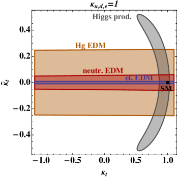
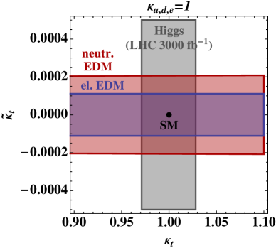
Figure 2: Left: Present constraints on $\kappa_{t}$ and $\tilde{\kappa}_{t}$ from the electron EDM (blue), the neutron EDM (red), the mercury EDM (brown), and Higgs physics (gray). Right: Projected future constraints on $\kappa_{t}$ and $\tilde{\kappa}_{t}$, see text for details.

The present constraints on $\kappa_{t}$ and $\tilde{\kappa}_{t}$ are shown in Fig. 2 (left). The regions allowed by the electron EDM, neutron EDM, mercury EDM, and collider constraints are colored in blue, red, brown, and gray, respectively, while the black point corresponds to the SM prediction. The constraints resulting from the EDM of the neutron and mercury employ the central values of the matrix elements in Eqs. (14) and (18). Note that the corrections to the $gg\to h$ and $h\to\gamma\gamma$ vertices scale differently with $\kappa_{t}$ and $\tilde{\kappa}_{t}$ and thus provide complementary constraints. The Higgs measurements are precise enough that they already by themselves constrain the CP-violating modification of the Higgs-top coupling to be below $\tilde{\kappa}_{t}\lesssim{\mathcal{O}}(0.5)$. The EDM constraints shrink the allowed region further to $\tilde{\kappa}_{t}\lesssim{\mathcal{O}}(0.01)$.

The right panel in Fig. 2 shows the prospects of the constraints. In order to obtain the plot we have assumed that $|d_{e}/e|<10^{-30}\,{\rm cm}$ Hewett:2012ns , a factor of $90$ improvement over the current best limit (6), and that $|d_{n}/e|<10^{-28}\,{\rm cm}$ Hewett:2012ns , a factor of 300 improvement with respect to the present bound (15). Our forecast for the future sensitivity of the Higgs production constraints is based on the results of the CMS study with a projection of errors to $3000$ fb^-1, which assumed $1/\sqrt{{\cal L}}$ scaling of the experimental uncertainties with luminosity ${\cal L}$, and also anticipates that the theory errors will be halved by then Olsen:talk:Seattle . In Fig. 2 we therefore take $\kappa_{g}=1.00\pm 0.03$ and $\kappa_{\gamma}=1.00\pm 0.02$ as the possible future fit inputs (centered around the SM predictions).

Since the EDMs depend linearly on $\tilde{\kappa}_{t}$, the projected order-of-magnitude improvements of the EDM constraints directly translate to order-of-magnitude improvements of the bounds on $\tilde{\kappa}_{t}$. For instance, the electron EDM is projected to be sensitive to values of $\tilde{\kappa}_{t}={\cal O}(10^{-4})$ which implies that one can probe scales up to $\Lambda={\cal O}(25\,{\rm TeV})$ for models (such as theories with top compositeness) where $\tilde{\kappa}_{t}\sim v^{2}/\Lambda^{2}$.

Note that the above EDM constraints rely heavily on the assumption that the Higgs couples to electrons, up, and down quarks. For illustration we assumed that these couplings are the same as in the SM. The possibility that the Higgs only couples to the third-generation fermions cannot be ruled out from current Higgs data. In this case there is no constraint from the electron EDM which is proportional to $\kappa_{e}\hskip 0.35565pt\tilde{\kappa}_{t}$. The neutron and mercury EDM are similarly dominated by the quark EDMs and CEDMs which scale as $\kappa_{u,d}\hskip 0.7113pt\tilde{\kappa}_{t}$. However, setting $\kappa_{u,d}=0$ the constraints due to $d_{n}$ and $d_{\rm Hg}$ do not vanish, because there is also a small contribution from the Weinberg operator which scales as $\kappa_{t}\hskip 0.35565pt\tilde{\kappa}_{t}$. In Fig. 3 we show the constraints for the limiting case where the Higgs only couples to the third-generation fermions. We see that at present ${\mathcal{O}(1)}$ values of $\tilde{\kappa}_{t}$ are allowed by the constraint from the neutron EDM. Assuming that only the Higgs-top couplings are modified, the Higgs data are then more constraining than the neutron EDM. This situation might change dramatically in the future with the expected advances in the measurement of the neutron EDM. As illustrated in Fig. 3 (right), a factor 300 improvement in the measurement of $d_{n}$ will lead to ${\mathcal{O}}(10^{-3})$ constraints on $\tilde{\kappa}_{t}$, making the neutron EDM as (or even more) powerful than the projected precision Higgs measurements at a high-luminosity upgrade of the LHC.

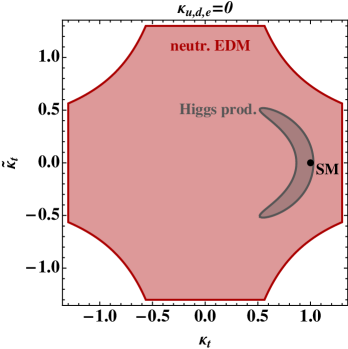
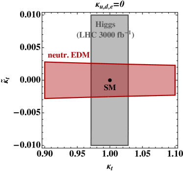
Figure 3: Left: Present constraints on $\kappa_{t}$ and $\tilde{\kappa}_{t}$ from the neutron EDM (red) and Higgs physics (gray), assuming that the Higgs only couples to the third generation. Right: Projected future constraints on $\kappa_{t}$ and $\tilde{\kappa}_{t}$, see text for details.

5 Constraints on bottom and tau couplings

In the following we analyze indirect and direct bounds on the couplings between the Higgs and the other two relevant third-generation fermions, i.e. the bottom quark and the tau lepton. In this case, the EDM constraints are suppressed by the small bottom and tau Yukawa couplings, which renders the present indirect limits weak. However, given the projected order-of-magnitude improvements in the experimental determinations of EDMs, relevant bounds are expected to arise in the future. We will see that these limits are complementary to the constraints that can be obtained via precision studies of Higgs properties at a high-luminosity LHC.

5.1 EDM constraints

The bottom-quark and tau-lepton loop contributions to the electron EDM are found from Eq. (3) after a simple replacement of charges and couplings. The calculation of the hadronic EDMs, on the other hand, is complicated by the appearance of large logarithms of the ratios $x_{f/h}\equiv m_{f}^{2}/M_{h}^{2}$ with $f=b,\tau$. The structure of the logarithmic corrections can be understood by evaluating Eqs. (10) and (11) in the limit $x_{f/h}\to 0$. In the bottom-quark case, we find

$$\begin{split}d_{q}(\mu_{W})&\simeq-4\hskip 0.7113pte\hskip 0.7113ptQ_{q}\hskip 0.7113ptN_{c}\hskip 0.7113ptQ_{b}^{2}\,\frac{\alpha}{(4\pi)^{3}}\hskip 0.7113pt\sqrt{2}G_{F}\hskip 0.7113ptm_{q}\,\kappa_{q}\tilde{\kappa}_{b}\,x_{b/h}\left(\ln^{2}x_{b/h}+\frac{\pi^{2}}{3}\right)\,,\\[5.69054pt] \tilde{d}_{q}(\mu_{W})&\simeq-2\,\frac{\alpha_{s}}{(4\pi)^{3}}\hskip 0.7113pt\sqrt{2}G_{F}\hskip 0.7113ptm_{q}\,\kappa_{q}\tilde{\kappa}_{b}\,x_{b/h}\left(\ln^{2}x_{b/h}+\frac{\pi^{2}}{3}\right)\,,\\[5.69054pt] w(\mu_{W})&\simeq-g_{s}\hskip 0.7113pt\frac{\alpha_{s}}{(4\pi)^{3}}\,\sqrt{2}G_{F}\,\kappa_{b}\tilde{\kappa}_{b}\,x_{b/h}\left(\ln x_{b/h}+\frac{3}{2}\right)\,.\end{split}$$ (34)

Here we have employed the asymptotic expansions $f_{1}(x)=x\left(\ln^{2}x+\pi^{2}/3\right)+{\cal O}(x^{2})$ and $f_{3}(x)=-4x\left(\ln x+3/2\right)+{\cal O}(x^{2})$ valid for $x\ll 1$. Note that $\tilde{d}_{q}$ is proportional to $\alpha_{s}\ln^{2}x_{b/h}$, whereas $w$ involves a term $\alpha_{s}\ln x_{b/h}$. This implies that only the coefficient $\tilde{d}_{q}$ leads to a leading logarithmic (LL) effect, while $w$ represents next-to-leading logarithmic (NLL) QCD corrections. In order to obtain reliable results for $d_{n}$ and $d_{\rm Hg}$ the logarithmic QCD effects in Eq. (34) have to be resummed to all orders in the strong coupling constant using the full machinery of RG-improved perturbation theory. We give details on this RG calculation in App. B. On the other hand, the double logarithm in $d_{q}$ arises from QED corrections and thus does not need to be resummed. In the appendix we calculate the LL QCD corrections to the quark EDM and show that they are larger than the QED effects given above. Therefore we will include both the leading QED and QCD contributions to $d_{q}$ in our numerical analysis.

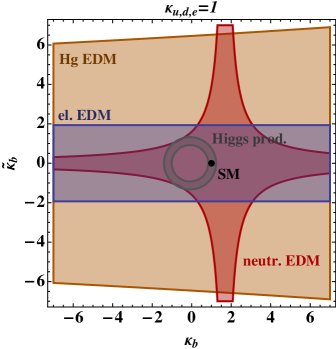
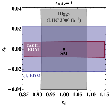
Figure 4: Left: Present constraints on $\kappa_{b}$ and $\tilde{\kappa}_{b}$ from the electron EDM (blue), the neutron EDM (red), the mercury EDM (brown), and Higgs physics (gray), restricting all other Higgs couplings to their SM values. Right: Possible future constraints on $\kappa_{b}$ and $\tilde{\kappa}_{b}$, see text for details.

Solving the relevant RG equations, we obtain the following approximate expressions for the case of the Higgs-bottom couplings $\kappa_{b}$ and $\tilde{\kappa}_{b}$:

$$\begin{split}\frac{d_{e}}{e}&=4.5\cdot 10^{-29}\,\tilde{\kappa}_{b}\,{\rm cm}\,,\\[5.69054pt] \frac{d_{n}}{e}&=\Big{\{}(1.0\pm 0.5)\left[-18.1\hskip 1.42262pt\tilde{\kappa}_{b}+0.15\hskip 1.42262pt\kappa_{b}\tilde{\kappa}_{b}\right]+(22\pm 10)\,0.48\hskip 1.42262pt\kappa_{b}\tilde{\kappa}_{b}\Big{\}}\cdot 10^{-27}\,{\rm cm}\,,\\[5.69054pt] \frac{d_{\rm Hg}}{e}&=-\left(4^{+8}_{-2}\right)\Big{[}0.12\hskip 1.42262pt\tilde{\kappa}_{b}-1.1\cdot 10^{-3}\hskip 1.42262pt\kappa_{b}\tilde{\kappa}_{b}\Big{]}\cdot 10^{-29}\,{\rm cm}\,.\end{split}$$ (35)

For the bottom-quark contribution to the electron EDM we take into account logarithmic effects associated to the running of the electromagnetic coupling constant by employing $\alpha\simeq 1/137$, renormalized at zero-momentum transfer, which is appropriate for real photon emission. In consequence, the above formula for $d_{e}$ is obtained from the result for $d_{q}$ in Eq. (34) by replacing $q\to e$ everywhere. Electromagnetic corrections describing operator mixing are, on the other hand, not included.

In the case of modified Higgs-tau couplings $\kappa_{\tau}$ and $\tilde{\kappa}_{\tau}$, we find

$$\begin{split}\frac{d_{e}}{e}&=3.7\cdot 10^{-29}\,{\rm cm}\,\tilde{\kappa}_{\tau}\,,\\[5.69054pt] \frac{d_{n}}{e}&=\left(1.0\pm 0.5\right)22.3\hskip 1.42262pt\tilde{\kappa}_{\tau}\cdot 10^{-29}\,{\rm cm}\,.\end{split}$$ (36)

Again no RG resummation of QED effects beyond the renormalization of the electric charge has been performed here. Numerically, this resummation is a ${\mathcal{O}}(10\%)$ correction for the neutron EDM, which is clearly a sub-leading effect given the present hadronic uncertainties in $d_{n}$. The expression for $d_{n}$ is obtained from $d_{q}$, as given in Eq. (34), by replacing $b\to\tau$ in all subscripts and setting $N_{c}\to 1$, while in the case of $d_{e}$ one in addition replaces $q\to e$ in all the subscripts. Since the mercury EDM does not provide a meaningful constraint on the couplings $\kappa_{\tau}$ and $\tilde{\kappa}_{\tau}$, we do not give an expression for $d_{\rm Hg}/e$.

5.2 Direct Higgs constraints

The modified Higgs-bottom couplings induce corrections to the effective $gg\to h$ and $h\to\gamma\gamma$ vertices of the following form

$$\begin{split}\kappa_{g}&\simeq\left(-0.05+0.08\hskip 1.42262pti\right)\kappa_{b}+1.05-0.08\hskip 1.42262pti\,,\qquad\hskip 14.22636pt\tilde{\kappa}_{g}\simeq\left(-0.06+0.08\hskip 1.42262pti\right)\tilde{\kappa}_{b}\,,\\[2.84526pt] \kappa_{\gamma}&\simeq\left(0.004-0.005\hskip 1.42262pti\right)\kappa_{b}+0.996+0.005\hskip 1.42262pti\,,\qquad\tilde{\kappa}_{\gamma}\simeq\left(0.004-0.005\hskip 1.42262pti\right)\tilde{\kappa}_{b}\,.\end{split}$$ (37)

The SM vertices in the two cases are dominated by the top-quark and $W$-boson couplings to the Higgs, both of which are ${\mathcal{O}}(1)$, and thus much larger than the SM bottom-quark Yukawa coupling $y_{b}={\cal O}(0.02)$. As a result the corrections in $\kappa_{g,\gamma}$ and $\tilde{\kappa}_{g,\gamma}$ due to $\kappa_{b}\neq 1$ and $\tilde{\kappa}_{b}\neq 0$ are sub-leading and can be neglected in our analysis (we have checked this explicitly).

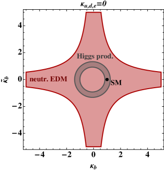
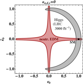
Figure 5: Left: Present constraints on $\kappa_{b}$ and $\tilde{\kappa}_{b}$ from the neutron EDM (red) and Higgs physics (gray), assuming that the Higgs only couples to the third-generation fermions, $W$, and $Z$ bosons. Right: Possible future constraints on $\kappa_{b}$ and $\tilde{\kappa}_{b}$, see text for details.

The most significant change in the Higgs signals arises therefore from the change in the total Higgs-decay width. Assuming that only the Higgs coupling to bottom quarks is modified, the new total decay width of the Higgs is

$$\Gamma=\left[1+\left(\kappa_{b}^{2}+\tilde{\kappa}_{b}^{2}-1\right){\rm Br}(h\to b\bar{b})_{\rm SM}\right]\Gamma_{\rm SM}\,\,.$$ (38)

This means that the $h\to b\bar{b}$ branching ratio is now

$${\rm Br}(h\to b\bar{b})=\frac{\left(\kappa_{b}^{2}+\tilde{\kappa}_{b}^{2}\right){\rm Br}(h\to b\bar{b})_{\rm SM}}{1+\left(\kappa_{b}^{2}+\tilde{\kappa}_{b}^{2}-1\right){\rm Br}(h\to b\bar{b})_{\rm SM}}\,,$$ (39)

while all the other Higgs-decay modes get rescaled to

$${\rm Br}(h\to X)=\frac{{\rm Br}(h\to X)_{\rm SM}}{1+\left(\kappa_{b}^{2}+\tilde{\kappa}_{b}^{2}-1\right){\rm Br}(h\to b\bar{b})_{\rm SM}}\,,$$ (40)

where $X\neq b\bar{b}$. As inputs we use the naive averages of the ATLAS ATLAS-CONF-2013-034 and CMS collaborations CMS-PAS-HIG-13-005 in different Higgs-decay channels

$$\begin{split}\hat{\mu}_{b\bar{b}}&=0.72\pm 0.53\,,\quad\hat{\mu}_{\tau\bar{\tau}}=1.02\pm 0.35\,,\quad\hat{\mu}_{\gamma\gamma}=1.14\pm 0.20\,,\\[5.69054pt] &\qquad\hat{\mu}_{WW}=0.78\pm 0.17\,,\quad\hat{\mu}_{ZZ}=1.11\pm 0.23\,,\end{split}$$ (41)

where $\hat{\mu}_{X}\equiv[\sigma(pp\to h)\hskip 1.42262pt{\rm Br}(h\to X)]/[\sigma(pp\to h)\hskip 1.42262pt{\rm Br}(h\to X)]_{\rm SM}$ denotes the signal strengths. We work in the limit where the Higgs couplings to the $W$ and $Z$ bosons are the SM ones. We keep the effect of $\kappa_{b},\tilde{\kappa}_{b}$ in the $gg\to h$ and $h\to\gamma\gamma$ vertices $\big{(}$cf. Eq. (37)$\big{)}$, where the former interaction also modifies the Higgs production cross section. Up to these sub-leading corrections the changes in the signal strengths are the same as in the corresponding branching ratios, Eqs. (39), (40), with $\hat{\mu}_{X}={\rm Br}(h\to X)/{\rm Br}(h\to X)_{\rm SM}$.

The resulting direct constraints in the $\kappa_{b}$–$\tilde{\kappa}_{b}$ plane are displayed in Fig. 4. As shown in the left panel, the present restrictions from Higgs physics carve out a ring-like allowed region that corresponds to effects of ${\cal O}(1)$ in $\kappa_{b}$ and $\tilde{\kappa}_{b}$. We also see that the EDMs currently impose even weaker bounds, with the strongest limit coming from $d_{n}$. However, the relative strength of the two sets of constraints is expected to change in the future, as illustrated in the right panel. For our forecast we use the CMS projections for a $h\to b\bar{b}$ coupling measurement with 3000 fb^-1 of integrated luminosity Olsen:talk:Seattle , assuming that this bounds the combination $\kappa_{b}^{2}+\tilde{\kappa}_{b}^{2}$. Including the constraints from the projected measurements of the $gg\to h$ and $h\to\gamma\gamma$ vertices breaks the symmetry between $\kappa_{b}$ and $\tilde{\kappa}_{b}$, so that only part of the ring-like region survives (we used the SM values for the central values of the hypothetical measurements). This limits the size of possible modifications in $\kappa_{b}$ to ${\cal O}(0.05)$. Complementary information is obtained in such a future scenario from the envisioned high-precision measurements of the electron and neutron EDM, which might allow to probe values of the CP-violating coefficient $\tilde{\kappa}_{b}$ down to ${\cal O}(10^{-2})$.

While the EDM constraints depicted in Fig. 4 assume that the Higgs couples to first-generation fermions with SM strength, meaningful EDM constraints on $\tilde{\kappa}_{b}$ can even emerge if $\kappa_{u,d}=0$. In fact, as illustrated in Fig. 5, the neutron EDM probes $\tilde{\kappa}_{b}$ through the Weinberg operator also if the Higgs couples only to the third generation. While at present (left panel) no relevant constraint can be derived in such a case, extracting a limit on $\tilde{\kappa}_{b}$ of ${\mathcal{O}}(0.1)$ may be possible in the future (right panel) if $\kappa_{b}$ is SM-like. This feature again highlights the power of low-energy EDM measurements in probing new sources of CP violation.

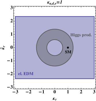
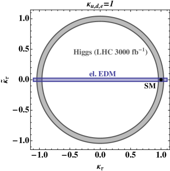
Figure 6: Left: Present constraints on $\kappa_{\tau}$ and $\tilde{\kappa}_{\tau}$ from the electron EDM (blue) and Higgs production (gray), assuming SM values for the remaining Higgs couplings. Right: Possible future constraints on $\kappa_{\tau}$ and $\tilde{\kappa}_{\tau}$, see text for details.

Modifying the Higgs-tau couplings changes the effective $h\to\gamma\gamma$ vertex. The induced shifts are parametrized by

$$\kappa_{\gamma}\simeq\left(0.004-0.003\hskip 1.42262pti\right)\kappa_{\tau}+0.996+0.003\hskip 1.42262pti\,,\qquad\tilde{\kappa}_{\gamma}\simeq\left(0.004-0.003\hskip 1.42262pti\right)\tilde{\kappa}_{\tau}\,.$$ (42)

Similar to the case of Higgs couplings to bottom quarks, the corrections to $\kappa_{\gamma}$ and $\tilde{\kappa}_{\gamma}$ are suppressed by the small tau Yukawa coupling, $y_{\tau}={\cal O}(0.01)$. The main effect is therefore the rescaling of the total decay widths, as in Eqs. (39), (40), but replacing $b\to\tau$. The resulting constraints in the $\kappa_{\tau}$–$\tilde{\kappa}_{\tau}$ plane are displayed in Fig. 6, with the left panel showing the current bounds, and the right panel the extrapolation to $3000$ fb^-1 of integrated luminosity, using again Olsen:talk:Seattle . One observes that even the projected precision of $2\%$ on $\kappa_{\gamma}$ will not suffice to break the symmetry between $\kappa_{\tau}$ and $\tilde{\kappa}_{\tau}$ and the ring-like bound persists, allowing for potentially ${\mathcal{O}}(1)$ values of the CP-violating modification $\tilde{\kappa}_{\tau}$. While at present the EDMs lead to a bound $|\tilde{\kappa}_{\tau}|\lesssim 2$, of the same order but slightly weaker than the collider constraint, assuming a factor of $90$ improvement in the determination of the electron EDM will change the situation, as it will make values $\tilde{\kappa}_{\tau}={\cal O}(10^{-2})$ accessible. Direct searches at the LHC using angular correlations in the $h\to\tau\bar{\tau}$ channel may be capable to probe $\tilde{\kappa}_{\tau}$ values of ${\cal O}(0.1)$ Berge:2008wi ; Berge:2008dr ; Berge:2011ij ; Fermilab:CPV , and are thus less powerful than the indirect bounds. Unlike the constraint from the electron EDM, direct bounds, however, do not depend on the assumption $\kappa_{e}=1$.

6 Conclusions

The LHC discovery of the Higgs boson furnishes new opportunities in the search for physics beyond the SM. Since in the SM the Higgs couplings to both gauge bosons and fermions are uniquely fixed in terms of the corresponding masses, finding a significant deviation from this simple pattern would constitute a clear signal of NP. In fact, a major experimental effort is directed towards determining the structure of the Higgs sector including its CP properties by measuring the various decay rates of the new boson as accurately as possible. While the current LHC results favor purely scalar-like Higgs-gauge boson interactions, searches for CP violation in fermionic Higgs decays are still in their fledgling stages.

In this article we have emphasized the complementarity between high-$p_{T}$ and low-energy precision measurements in extracting information about the CP properties of the Higgs-boson couplings to third-generation fermions. In the case of the Higgs-top couplings we find that the existing data on Higgs production and decay are already precise enough to constrain the CP-violating modification to $\tilde{\kappa}_{t}\lesssim{\cal O}(0.5)$. The present constraints arising from the EDMs shrink the allowed region further to $\tilde{\kappa}_{t}={\cal O}(0.01)$, if SM couplings of the Higgs to the first generation fermions are assumed. At a high-luminosity LHC and the next generation of EDM experiments it should be possible to improve the above limits on CP violation in the Higgs-top coupling significantly. Our analysis shows that while at the 14 TeV LHC with $3000\,{\rm fb}^{-1}$ of integrated luminosity a sensitivity of $\tilde{\kappa}_{t}={\cal O}(10^{-2})$ can be reached, the electron EDM is projected to be sensitive to values down to $\tilde{\kappa}_{t}={\cal O}(10^{-4})$. Such a precision will allow to indirectly probe for NP scales up to $\Lambda={\cal O}(25\,{\rm TeV})$ in models, such as theories with top compositeness, that predict $\tilde{\kappa}_{t}\sim v^{2}/\Lambda^{2}$.

The above EDM bounds on $\tilde{\kappa}_{t}$ only apply under the assumption that the electron and the down- and up-quark Yukawa couplings take their SM values. This requirement can be avoided, however. The constraints due to the neutron and mercury EDM do not vanish even if the Higgs boson couples only to the third generation of fermions, because there is a small contribution from the Weinberg operator proportional to the product $\kappa_{t}\tilde{\kappa}_{t}$. Our numerical study shows that a factor 300 improvement in the measurement of the neutron EDM will lead to ${\mathcal{O}}(10^{-3})$ constraints on $\tilde{\kappa}_{t}$ from the Weinberg operator alone (and will thus not dependent on assumptions about the Higgs couplings to the first generation fermions). This sensitivity exceeds the projected precision of the Higgs-boson measurements at a high-luminosity upgrade of the LHC.

In the case of the Higgs-bottom and -tau couplings we find that the present LHC Higgs data permit ${\cal O}(1)$ modifications in $\kappa_{b,\tau}$ and $\tilde{\kappa}_{b,\tau}$. While the EDMs currently impose even weaker bounds, the situation may be reversed in the future. With $3000\,{\rm fb}^{-1}$ of integrated luminosity the LHC should be able to constrain ${\cal O}(0.05)$ values of $\kappa_{b}$, while the sensitivity of the proposed EDM measurements reaches ${\cal O}(10^{-2})$ for $\tilde{\kappa}_{b}$, if the Higgs boson couples to the first generation with SM strength. Assuming that the Higgs does only interact with the third generation, extracting a limit from the neutron EDM on $\tilde{\kappa}_{b}$ of ${\cal O}(0.05)$ should still be possible. In the case of the Higgs-tau couplings, we saw that even the full high-luminosity LHC data set will allow for $\tilde{\kappa}_{\tau}={\cal O}(1)$. Using angular correlations in the $h\to\tau\bar{\tau}$ channel, direct searches at the LHC may be capable to probe $\tilde{\kappa}_{\tau}$ values of ${\cal O}(0.1)$ Berge:2008wi ; Berge:2008dr ; Berge:2011ij ; Fermilab:CPV . A possible improvement by three orders of magnitudes in the determination of the electron EDM will, on the other hand, make values $\tilde{\kappa}_{\tau}={\cal O}(10^{-2})$ accessible, if the Higgs couples to the electron.

Appendix A RG analysis for neutron EDM

In order to estimate the size of the neutron EDM one has to perform a RG analysis including the effects of operator mixing. The mixing of the three operators

$$\begin{split}{\cal Q}_{1}^{q}&=-\frac{i}{2}\hskip 0.7113pte\,Q_{q}\,m_{q}\,\bar{q}\hskip 0.7113pt\sigma^{\mu\nu}\gamma_{5}\hskip 0.7113ptq\,F_{\mu\nu}\,,\\[2.84526pt] {\cal Q}_{2}^{q}&=-\frac{i}{2}\hskip 0.7113ptg_{s}m_{q}\,\bar{q}\hskip 0.7113pt\sigma^{\mu\nu}T^{a}\gamma_{5}\hskip 0.7113ptq\,G^{a}_{\mu\nu}\,,\\[2.84526pt] {\cal Q}_{3}&=-\frac{1}{3}\hskip 0.7113ptg_{s}\hskip 0.7113ptf^{abc}\,G_{\mu\sigma}^{a}G_{\nu}^{b,\sigma}\widetilde{G}^{c,\mu\nu}\,,\end{split}$$ (43)

has been given in Braaten:1990gq ; Degrassi:2005zd . In this normalization the Wilson coefficients at the high scale read

$$\begin{split}{\cal C}_{1}^{q}(\mu_{W})&=-\frac{16}{3}\frac{\alpha}{(4\pi)^{3}}\hskip 0.7113pt\sqrt{2}G_{F}\,\kappa_{q}\tilde{\kappa}_{t}\hskip 1.42262ptf_{1}(x_{t/h})\,,\\[2.84526pt] {\cal C}_{2}^{q}(\mu_{W})&=-2\hskip 0.7113pt\,\frac{\alpha_{s}}{(4\pi)^{3}}\hskip 0.7113pt\sqrt{2}G_{F}\,\kappa_{q}\tilde{\kappa}_{t}\hskip 1.42262ptf_{1}(x_{t/h})\,,\\[2.84526pt] {\cal C}_{3}(\mu_{W})&=\frac{1}{4}\frac{\alpha_{s}}{(4\pi)^{3}}\,\sqrt{2}G_{F}\,\kappa_{t}\hskip 0.7113pt\tilde{\kappa}_{t}\,f_{3}(x_{t/h})\,,\end{split}$$ (44)

where $\alpha$ and $\alpha_{s}$ are understood to be evaluated at the scale $\mu_{W}={\cal O}(m_{t})$. By solving the RG equations

$$\mu\hskip 1.42262pt\frac{d}{d\mu}\,\vec{{\cal C}}(\mu)=\gamma^{T}\,\vec{{\cal C}}(\mu)\,,\qquad\vec{{\cal C}}(\mu)=\big{(}{\cal{C}}_{1}^{q}(\mu),{\cal{C}}_{2}^{q}(\mu),{\cal{C}}_{3}(\mu)\big{)}^{T}\,,$$ (45)

using the leading-order (LO) anomalous dimension matrix (ADM)

$$\gamma=\frac{\alpha_{s}}{4\pi}\begin{pmatrix}\frac{32}{3}&\phantom{-}0&0\\[5.69054pt] \frac{32}{3}&\phantom{-}\frac{28}{3}&0\\[5.69054pt] 0&-6&14+\frac{4N_{f}}{3}\end{pmatrix}\,,$$ (46)

with $N_{f}$ denoting the number of active flavors, one resums LL effects and can determine the Wilson coefficients at the hadronic scale $\mu_{H}$.

In Pospelov:2005pr a normalization of the three operators for calculating their matrix elements is used that differs from Braaten:1990gq ; Degrassi:2005zd , namely

$${\cal Q}_{e}^{q}=\frac{{\cal Q}_{1}^{q}}{e}\,,\qquad{\cal Q}_{c}^{q}={\cal Q}_{2}^{q}\,,\qquad{\cal Q}_{G}=\frac{{\cal Q}_{3}}{g_{s}}\,.$$ (47)

In the latter basis, the Wilson coefficients at the high scale are given by

$${\cal C}_{e}^{q}(\mu_{W})=e\hskip 1.42262pt{\cal C}_{1}^{q}(\mu_{W})\,,\qquad{\cal C}_{c}^{q}(\mu_{W})={\cal C}_{2}^{q}(\mu_{W})\,,\qquad{\cal C}_{G}(\mu_{W})=g_{s}(\mu_{W})\hskip 1.42262pt{\cal C}_{3}(\mu_{W})\,.$$ (48)

The new Wilson coefficients (48) can be obtained from the old ones (44) by the simple redefinition $g_{s}(\mu_{H})\,{\cal C}_{3}(\mu_{W})=\eta^{-1/2}\,{\cal C}_{G}(\mu_{W})$ with $\eta=\alpha_{s}(\mu_{W})/\alpha_{s}(\mu_{H})$. Performing five- and four-flavor running, we find in the new basis

$$\begin{split}{\cal C}_{e}^{q}(\mu_{H})&=0.45\,{\cal C}_{e}^{q}(\mu_{W})-0.38\;{\cal C}_{c}^{q}(\mu_{W})-0.07\;\frac{{\cal C}_{G}(\mu_{W})}{g_{s}(\mu_{W})}\,,\\[2.84526pt] {\cal C}_{c}^{q}(\mu_{H})&=0.50\,{\cal C}_{c}^{q}(\mu_{W})+0.15\;\frac{{\cal C}_{G}(\mu_{W})}{g_{s}(\mu_{W})}\,,\\[8.53581pt] {\cal C}_{G}(\mu_{H})&=0.40\,{\cal C}_{G}(\mu_{W})\,.\end{split}$$ (49)

The above low-energy Wilson coefficients are related to the dipole moments $d_{q}$, $\tilde{d}_{q}$, and the coefficient $w$ as follows

$$d_{q}=\hskip 0.7113ptQ_{q}\hskip 0.7113ptm_{q}\,C_{e}^{q}(\mu_{H})\,,\qquad\tilde{d}_{q}=m_{q}\,C_{c}^{q}(\mu_{H})\,,\qquad w=C_{G}(\mu_{H})\,.$$ (50)

We now set $\mu_{W}=m_{t}$, $\mu_{H}=1\,{\rm GeV}$, and use $\alpha_{s}(m_{t})=0.109$, $\alpha_{s}(\mu_{H})=0.36$, $m_{u}(\mu_{H})=2.4\cdot 10^{-3}\,{\rm GeV}$, and $m_{d}(\mu_{H})=5.4\cdot 10^{-3}\,{\rm GeV}$. These numerical values are obtained from the input given in Beringer:1900zz and Laiho:2011rb , by employing one-loop running of the strong coupling constant and the quark masses. In this way, we arrive at

$$\begin{split}\frac{d_{n}}{e}&=\Big{\{}(1.0\pm 0.5)\left[-(1.0\hskip 0.7113pt\kappa_{u}+4.3\hskip 0.7113pt\kappa_{d})\hskip 1.42262pt\tilde{\kappa}_{t}+5.1\cdot 10^{-2}\hskip 1.42262pt\kappa_{t}\tilde{\kappa}_{t}\right]\\[8.53581pt] &\phantom{xxx}+(22\pm 10)\,1.8\cdot 10^{-2}\hskip 1.42262pt\kappa_{t}\tilde{\kappa}_{t}\Big{\}}\cdot 10^{-25}\,{\rm cm}\,,\end{split}$$ (51)

where we kept the couplings to up and down quarks explicit. This result generalizes the expression given in (14).

Appendix B Bottom-quark contributions to neutron EDM

In Sec. 5.1 we have argued that integrating out the bottom quark together with the Higgs boson at the electroweak scale introduces a large scale uncertainty. The situation can be remedied by removing the Higgs and the bottom quark as active degrees of freedoms in two steps and using RG-improved perturbation theory to resum the logarithms in the expansions (34) of the full results.

In a first step we integrate out the Higgs boson at the scale $\mu_{W}={\cal O}(M_{h})$, which leads to an effective five-flavor theory. The corresponding Lagrangian is given in terms of the following operators

$$\begin{split}O_{1}^{q}&=\bar{q}q\,\bar{b}\hskip 0.7113pti\gamma_{5}\hskip 0.7113ptb\,,\\[5.69054pt] O_{2}^{q}&=\bar{q}\hskip 1.42262ptT^{a}\hskip 0.35565ptq\,\bar{b}\hskip 0.7113pti\gamma_{5}T^{a}\hskip 0.7113ptb\,,\\[5.69054pt] O_{3}^{q}&=\bar{q}\hskip 0.7113pt\sigma_{\mu\nu}\hskip 0.7113ptq\,\bar{b}\hskip 0.7113pti\sigma^{\mu\nu}\gamma_{5}\hskip 0.7113ptb\,,\\[5.69054pt] O_{4}^{q}&=\bar{q}\hskip 0.7113pt\sigma_{\mu\nu}T^{a}\hskip 0.7113ptq\,\bar{b}\hskip 0.7113pti\sigma^{\mu\nu}\gamma_{5}T^{a}\hskip 0.7113ptb\,,\\[5.69054pt] O_{5}^{q}&=-\frac{i}{2}\hskip 0.7113pte\hskip 0.7113ptQ_{b}\hskip 0.7113pt\frac{m_{b}}{g_{s}^{2}}\,\bar{q}\hskip 0.7113pt\sigma^{\mu\nu}\gamma_{5}\hskip 0.7113ptq\hskip 1.42262ptF_{\mu\nu}\,,\\ O_{6}^{q}&=-\frac{i}{2}\hskip 0.7113pt\frac{m_{b}}{g_{s}}\,\bar{q}\hskip 0.7113pt\sigma^{\mu\nu}T^{a}\gamma_{5}\hskip 0.7113ptq\hskip 1.42262ptG^{a}_{\mu\nu}\,,\\ O_{7}&=-\frac{1}{3\hskip 0.35565ptg_{s}}\hskip 0.7113ptf^{abc}\,G_{\mu\sigma}^{a}G_{\nu}^{b,\sigma}\widetilde{G}^{c,\mu\nu}\,,\end{split}$$ (52)

by

$$\begin{split}{\mathcal{L}}_{\text{eff}}=-\frac{\sqrt{2}G_{F}}{M_{h}^{2}}\,m_{b}\hskip 0.7113pt\tilde{\kappa}_{b}\,\bigg{\{}&\sum_{q=u,d}m_{q}\hskip 0.7113pt\kappa_{q}\sum_{i=1,2,3,4,5,6}C_{i}^{q}\hskip 0.7113ptO_{i}^{q}\\[5.69054pt] &+m_{b}\hskip 0.7113pt\kappa_{b}\,\bigg{[}\,\sum_{j=1,3,5,6}C_{j}^{b}\hskip 0.7113ptO_{j}^{b}+C_{7}\hskip 0.7113ptO_{7}\,\bigg{]}\bigg{\}}\,.\end{split}$$ (53)

Notice that the above operators are normalized in such a way that operator mixing starts at $\mathcal{O}(\alpha_{s})$, $\gamma=\alpha_{s}/(4\pi)\,\gamma^{(0)}+(\alpha_{s}/(4\pi))^{2}\,\gamma^{(1)}+{\cal O}(\alpha_{s}^{3})$. The Wilson coefficients $C_{5}^{q}$, $C_{6}^{q}$, and $C_{7}$ are related to $d_{q}$, $\tilde{d}_{q}$, and $w$ by

$$\begin{split}d_{q}(\mu)&=-\frac{e\hskip 0.7113ptQ_{b}}{4\pi\alpha_{s}}\,\sqrt{2}G_{F}\hskip 0.7113ptm_{q}\,\kappa_{q}\tilde{\kappa}_{b}\,x_{b/h}\,C_{5}^{q}(\mu)\,,\\[5.69054pt] \tilde{d}_{q}(\mu)&=-\frac{1}{4\pi\alpha_{s}}\,\sqrt{2}G_{F}\hskip 0.7113ptm_{q}\,\kappa_{q}\tilde{\kappa}_{b}\,x_{b/h}\,C_{6}^{q}(\mu)\,,\\[5.69054pt] w(\mu)&=-\frac{g_{s}}{4\pi\alpha_{s}}\,\sqrt{2}G_{F}\hskip 0.7113pt\kappa_{b}\tilde{\kappa}_{b}\,x_{b/h}\,C_{7}(\mu)\,.\end{split}$$ (54)

    

Figure 7: Left: The diagram in the full theory that gives rise to the LO matching correction to $C_{1}^{q}$. The same graph with the quarks $q$ replaced by a bottom quarks $b$ induces a non-zero initial condition for $C_{1}^{b}$. Middle: An example of a graph that contributes to the one-loop mixing of $O_{1}^{q}$ into $O_{4}^{q}$. Right: Feynman diagram describing the one-loop mixing of $O_{4}^{q}$ into $O_{6}^{q}$. The shown graph involves a closed bottom-quark line. See text for further explanations.

We perform the RG running between $\mu_{W}$ and the bottom-quark threshold $\mu_{b}={\cal O}(m_{b})$ employing the operator basis

$$\vec{O}=(O_{1}^{q},O_{2}^{q},O_{3}^{q},O_{4}^{q},O_{1}^{b},O_{3}^{b},O_{5}^{q},O_{6}^{q},O_{5}^{b},O_{6}^{b},O_{7})^{T}\,,$$ (55)

with $q=u,d$. At the tree level only the Wilson coefficients of $O_{1}^{q}$ and $O_{1}^{b}$ receive a non-zero initial condition, cf. Fig. 7 (left). In our normalization the corresponding matching coefficients read

$$\vec{C}^{\,(0)}(\mu_{W})=(1,0,0,0,1,0,0,0,0,0,0)^{T}\,.$$ (56)

Adapting existing results for the anomalous dimensions Braaten:1990gq ; Degrassi:2005zd ; Borzumati:1999qt ; Buras:2000if ; Hisano:2012cc to our definition of operators (52), we find for the LO ADM in the effective five-flavor theory

$$\gamma^{(0)}=\setcounter{MaxMatrixCols}{11}\begin{pmatrix}-16&0&0&-2&0&0&0&0&0&0&0\\[5.69054pt] 0&2&-\frac{4}{9}&-\frac{5}{6}&0&0&0&0&0&0&0\\[5.69054pt] 0&-96&\frac{16}{3}&0&0&0&-48&0&0&0&0\\[5.69054pt] -\frac{64}{3}&-40&0&-\frac{38}{3}&0&0&0&-8&0&0&0\\[5.69054pt] 0&0&0&0&-10&-\frac{1}{6}&0&0&4&4&0\\[5.69054pt] 0&0&0&0&40&\frac{34}{3}&0&0&-112&-16&0\\[5.69054pt] 0&0&0&0&0&0&-\frac{14}{3}&0&0&0&0\\[5.69054pt] 0&0&0&0&0&0&\frac{32}{3}&-6&0&0&0\\[5.69054pt] 0&0&0&0&0&0&0&0&-\frac{14}{3}&0&0\\[5.69054pt] 0&0&0&0&0&0&0&0&\frac{32}{3}&-6&0\\[5.69054pt] 0&0&0&0&0&0&0&-6&0&-6&\frac{16}{3}\end{pmatrix}\,.$$ (57)

Notice that the operators $O_{1}^{b}$ and $O_{3}^{b}$ only mix among themselves at the one-loop level. This implies that they do not affect the resummation of the LL QCD contributions to $C_{5}^{q}$ and $C_{6}^{q}$. The one-loop mixing of $O_{1}^{b}$ and $O_{3}^{b}$ plays however an important role in the calculation of the NLL corrections to $C_{7}$.

We first discuss the resummation of logarithms for the Wilson coefficient of $O_{6}^{q}$. By solving the usual RG equations $\big{(}$see Eq. (45)$\big{)}$, we obtain in terms of $\eta_{5}\equiv\alpha_{s}(\mu_{W})/\alpha_{s}(\mu_{b})$, the following expression

$$\begin{split}C_{6}^{q}(\mu_{b})&=\frac{432}{2773\hskip 1.42262pt\eta_{5}^{9/23}}+\frac{0.07501}{\eta_{5}^{1.414}}+9.921\cdot 10^{-4}\hskip 1.42262pt\eta_{5}^{0.7184}-\frac{0.2670}{\eta_{5}^{0.6315}}+\frac{0.03516}{\eta_{5}^{0.06417}}+{\cal O}(\alpha_{s}^{3})\\[5.69054pt] &\simeq\bigg{(}\frac{\alpha_{s}}{4\pi}\bigg{)}^{2}\,\frac{\gamma_{14}^{(0)}\gamma_{48}^{(0)}}{8}\,\ln^{2}x_{b/h}+{\cal O}(\alpha_{s}^{3})\,,\end{split}$$ (58)

for the Wilson coefficient of the CEDM operator. Notice that the final result only contains the LL correction which is proportional to the combination $\gamma_{14}^{(0)}\gamma_{48}^{(0)}$ of one-loop anomalous dimensions (cf. (57)). Inserting (58) into (54) we recover the result for $\tilde{d}_{q}$ as given in Eq. (34). Diagrammatically the LL bottom-quark corrections to the CEDM therefore arise from the mixing $O_{1}^{q}\to O_{4}^{q}$ followed by $O_{4}^{q}\to O_{6}^{q}$, cf. Fig. 7 (middle and right). Employing $\mu_{W}=M_{h}$ and $\mu_{b}=m_{b}=4.2\,{\rm GeV}$ with $\alpha_{s}(M_{h})=0.113$ and $\alpha_{s}(m_{b})=0.212$, we find numerically $C_{6}^{q}(m_{b})=0.008\;(0.026)$ for the last line in Eq. (58) using $\alpha_{s}=\alpha_{s}(M_{h})$ $\big{(}$$\alpha_{s}=\alpha_{s}(m_{b})$$\big{)}$. The resummed result is $C_{6}^{q}(m_{b})=0.022$, which shows that the resummation of QCD logarithms is phenomenologically important for the CEDM $\tilde{d}_{q}$.

The Wilson coefficient of the operator $O_{5}^{q}$ receives both QED and QCD corrections. Including the ${\cal O}(\alpha)$ contributions to $d_{q}$ as given in Eq. (34) in their unresummed form, but resumming the LL QCD effects, we obtain

$$\begin{split}C_{5}^{q}(\mu_{b})&=-4\,\frac{\alpha\hskip 0.7113pt\alpha_{s}}{(4\pi)^{2}}\,Q_{q}\left(\ln^{2}x_{b/h}+\frac{\pi^{2}}{3}\right)+\frac{2688}{2773\hskip 1.42262pt\eta_{5}^{7/23}}-\frac{3456}{2773\hskip 1.42262pt\eta_{5}^{9/23}}\\[5.69054pt] &\phantom{xx}-\frac{0.03467}{\eta_{5}^{1.414}}+0.01407\hskip 1.42262pt\eta_{5}^{0.7184}+\frac{0.4102}{\eta_{5}^{0.6315}}-\frac{0.1126}{\eta_{5}^{0.06417}}+{\cal O}(\alpha_{s}^{4})\\[8.53581pt] &\simeq-4\,\frac{\alpha\hskip 0.7113pt\alpha_{s}}{(4\pi)^{2}}\,Q_{q}\ln^{2}x_{b/h}+\bigg{(}\frac{\alpha_{s}}{4\pi}\bigg{)}^{3}\,\frac{\gamma_{14}^{(0)}\gamma_{48}^{(0)}\gamma_{87}^{(0)}}{48}\,\ln^{3}x_{b/h}+{\cal O}(\alpha_{s}^{4})\,.\end{split}$$ (59)

One observes that the leading QCD contribution to $C_{5}^{q}$ is of ${\cal O}(\alpha_{s}^{3}\hskip 0.7113pt\ln^{3}x_{b/h})$ and proportional to the product $\gamma_{14}^{(0)}\gamma_{48}^{(0)}\gamma_{87}^{(0)}$ of the elements of the LO ADM (57). The LL QCD effects are hence formally of three-loop order, cf. Fig. 8 (left). It follows that the ratio between QCD and QED effects in $C_{5}^{q}$ is approximately given by

$$-\frac{2\hskip 0.7113pt\alpha_{s}^{2}}{9\pi\hskip 0.7113ptQ_{q}\hskip 0.7113pt\alpha}\,\ln x_{b/h}\simeq\frac{3.0}{Q_{q}}\,.$$ (60)

This shows that for $q=u$ ($q=d$) QCD corrections dominate over the QED effects by a factor of around $4.5$ ($-9.0$). In our numerical analysis we therefore employ the full result for the Wilson coefficient $C_{5}^{q}$ as given in the first two lines of Eq. (59).

Figure 8: Left: An example of a three-loop diagram involving an insertion of $O_{1}^{q}$ that gives rise to a logarithm of the form $\alpha_{s}^{3}\ln^{3}x_{b/h}$ in the Wilson coefficient $C_{5}^{q}$. Right: A two-loop graph describing the mixing of $O_{1}^{b}$ into $O_{7}$. For further details see text.

In the case of the coefficient $w$ of the Weinberg operator the resummation of the logarithmically-enhanced corrections in Eq. (34) is slightly more involved as it requires the knowledge of one- and two-loop anomalous dimensions. However, since only the initial condition for $Q_{1}^{b}$ is non-vanishing at LO, the only element needed from the ${\cal O}(\alpha_{s}^{2})$ ADM to resum the $\alpha_{s}\ln x_{b/h}$ term in $w$ is $\gamma_{5,11}^{(1)}$. This element describes the mixing of the operator $O_{1}^{b}$ into $O_{7}$, cf. Fig. 8 (right). From the LL-expanded expression for $w$, i.e. Eq. (34), we obtain $\gamma_{5,11}^{(1)}=2$. To gain full control over the order $\alpha_{s}^{3}\ln^{2}x_{b/h}$ terms in the Wilson coefficient $C_{7}$ requires also the knowledge of the element $\gamma_{6,11}^{(1)}$ of the two-loop ADM. By performing an explicit calculation we find that $\gamma_{6,11}^{(1)}=0$. Solving the RG equations then gives the full two-loop result

$$\begin{split}C_{7}(\mu_{b})&=\frac{\alpha_{s}(\mu_{b})}{4\pi}\left(\frac{4200}{659}\hskip 1.42262pt\eta_{5}^{31/23}+0.3176\hskip 1.42262pt\eta_{5}^{0.7184}-\frac{6.691}{\eta_{5}^{0.6315}}\right)\cdot 10^{-2}+{\cal O}(\alpha_{s}^{3})\\[8.53581pt] &\simeq\bigg{(}\frac{\alpha_{s}}{4\pi}\bigg{)}^{2}\,\frac{\gamma_{5,11}^{(1)}}{2}\,\ln x_{b/h}+{\cal O}(\alpha_{s}^{3})\,.\end{split}$$ (61)

Using Eq. (54), we recover from the final expression the NLL contribution to $w$ as reported in Eq. (34). Comparing the leading term in the expansion to the resummed result, we find $C_{7}(m_{b})=-0.6\cdot 10^{-3}\;(-2.0\cdot 10^{-3})$ for the last line in Eq. (61) employing $\alpha_{s}=\alpha_{s}(M_{h})$ $\big{(}\alpha_{s}=\alpha_{s}(m_{b})\big{)}$, while the RG-improved result is $C_{7}(m_{b})=-1.2\cdot 10^{-3}$. One observes again that for an accurate description of the effects associated to the Weinberg operator an RG analysis is mandatory.

Below the bottom-quark threshold one has to switch to the four-flavor theory by integrating out the $b$ quark. We use the following reduced set of operators

$$\vec{O}=\left(\frac{m_{q}}{m_{b}}\,O_{5}^{q},\frac{m_{q}}{m_{b}}\,O_{6}^{q},O_{7}\right)^{T}\,,$$ (62)

for which the corresponding LO ADM reads Degrassi:2005zd

$$\gamma^{(0)}=\begin{pmatrix}-6&0&0\\[5.69054pt] \frac{32}{3}&-\frac{22}{3}&0\\[5.69054pt] 0&-6&\frac{8}{3}\end{pmatrix}\,.$$ (63)

The tree-level matching for the Wilson coefficients $C_{5}^{q}(\mu_{b})$ and $C_{6}^{q}(\mu_{b})$ is trivial, but at the one-loop level the CEDM operator $O_{6}^{b}$ induces a finite threshold correction $\delta C_{7}(\mu_{b})$ to the Wilson coefficient of the Weinberg operator when the bottom quark is integrated out Chang:1990jv . The relevant one-loop graphs are shown in Fig. 9. We have

$$\delta C_{7}(\mu_{b})=\frac{\alpha_{s}(\mu_{b})}{8\pi}\,C_{6}^{b}(\mu_{b})\,,$$ (64)

with

$$C_{6}^{b}(\mu_{b})=\frac{50}{47\hskip 1.42262pt\eta_{5}^{9/23}}+3.969\cdot 10^{-3}\hskip 1.42262pt\eta_{5}^{0.7184}-\frac{1.0678}{\eta_{5}^{0.6315}}+{\cal O}(\alpha_{s}^{3})\,.$$ (65)

Solving the RG equations, we then obtain for the Wilson coefficients at the hadronic scale $\mu_{H}$ the following expressions

$$\begin{split}C_{5}^{q}(\mu_{H})&=\eta_{4}^{-9/25}\,C_{5}^{q}(\mu_{b})+8\left(\eta_{4}^{-9/25}-\eta_{4}^{-11/25}\,\right)C_{6}^{q}(\mu_{b})\\[5.69054pt] &\phantom{xx}+\left(\frac{72}{13}\,\eta_{4}^{-9/25}-\frac{24}{5}\,\eta_{4}^{-11/25}-\frac{48}{65}\,\eta_{4}^{4/25}\,\right)\frac{\kappa_{b}}{\kappa_{q}}\,C_{7}(\mu_{b})\,,\\[8.53581pt] C_{6}^{q}(\mu_{H})&=\eta_{4}^{-11/25}\,C_{6}^{q}(\mu_{b})+\frac{3}{5}\left(\eta_{4}^{-11/25}-\eta_{4}^{4/25}\,\right)\frac{\kappa_{b}}{\kappa_{q}}\,C_{7}(\mu_{b})\,,\\[8.53581pt] C_{7}(\mu_{H})&=\eta_{4}^{4/25}\,\Big{(}C_{7}(\mu_{b})+\delta C_{7}(\mu_{b})\Big{)}\,.\end{split}$$ (66)

Here $\eta_{4}\equiv\alpha_{s}(\mu_{b})/\alpha_{s}(\mu_{H})$ and the results for $C_{5}^{q}(\mu_{b})$, $C_{6}^{q}(\mu_{b})$, $C_{7}(\mu_{b})$, and $\delta C_{7}(\mu_{b})$ were given previously in Eqs. (59), (58), (61), and (64). Notice that we have included the $\delta C_{7}(\mu_{b})$ contribution only in the case of $C_{7}(\mu_{H})$, since it gives a $\alpha_{s}^{3}\ln^{2}x_{b/h}$ correction, which corresponds to a sub-leading logarithm in the case of $C_{5}^{q}(\mu_{H})$ and $C_{6}^{q}(\mu_{H})$.

Figure 9: One-loop diagrams leading to a correction to the Weinberg operator at the bottom-quark threshold. The black square denotes the insertion of the operator $O_{6}^{b}$. For further details consult the text.

Appendix C Other low-energy constraints

In this appendix we consider constraints on the modifications of the Higgs couplings to third-generation fermions that arise from low-energy probes other than the EDMs. Although the constraints discussed below turn out to be not very restrictive, we still mention them for completeness.

We begin our survey in the quark-flavor sector. Naively one might expect that the Higgs exchange in two-loop diagrams, cf. Fig. 10 (left), would lead to a CP-violating contribution to $B_{s}$–$\bar{B}_{s}$ mixing. Due to the symmetric nature of the diagrams, however, there is no correction proportional to $\kappa_{t}\hskip 0.7113pt\tilde{\kappa}_{t}$ at the level of dimension-six operators (we checked this through an explicit calculation). The contributions proportional to $\kappa_{t}\hskip 0.7113pt\tilde{\kappa}_{t}$ do arise beyond dimension six. As such they are suppressed by light quark masses and thus unobservable in practice. In consequence, CP violation in $B_{s}$–$\bar{B}_{s}$ mixing does not provide any relevant constraints on the modifications of the Higgs-top couplings.

    

Figure 10: Left: An example of a two-loop contribution to $B_{s}$–$\bar{B}_{s}$ mixing. Right: One-loop contribution to the magnetic dipole moment of the top quark. See text for details.

Constraints on $\kappa_{t}$ and $\tilde{\kappa}_{t}$ in principle arise also from the inclusive $B\to X_{s}\gamma$ decay at the two-loop level. The resulting bounds can be estimated by calculating the magnetic dipole moment of the top quark that is induced by Higgs exchange as shown in Fig. 10 (right). Inserting the effective top-photon interaction into the two one-loop graphs in which the photon is emitted from the internal top-quark line, i.e. those with $W$-boson and would-be Goldstone boson exchange, then leads to a contribution to $b\to s\gamma$. Performing such an analysis one finds that effects of ${\cal O}(100)$ in $\kappa_{t}$ and $\tilde{\kappa}_{t}$ are not in conflict with $B\to X_{s}\gamma$. Notice that an explicit two-loop calculation of $B\to X_{s}\gamma$ would e.g. also involve diagrams with $hWW$ vertices that are not included in our estimate. However, we expect that a complete ${\cal O}(\alpha^{2})$ calculation would not change our general conclusions.

If the Higgs-fermion interactions are modified according to Eq. (1) the one-loop amplitude of the $b\to sh$ transition is altered. Such a modification will change the prediction for the branching ratio of $B_{s}\to\mu^{+}\mu^{-}$. Allowing for a shift in ${\rm Br}\left(B_{s}\to\mu^{+}\mu^{-}\right)$ of $10^{-9}$ one can derive that values of ${\cal O}(100)$ of both $\kappa_{t}$ and $\tilde{\kappa}_{t}$ are consistent with the latter constraint.

In the case of $\kappa_{\tau}\neq 1$ and $\tilde{\kappa}_{\tau}\neq 0$, one-loop Higgs exchange will modify the prediction for the anomalous magnetic moment $a_{\tau}$ of the tau lepton. Modifications of ${\cal O}(10)$ in the Higgs-tau couplings can be shown to result in shifts in $a_{\tau}$ of ${\cal O}(10^{-8})$, i.e. effects comparable to the present SM uncertainty. Given that the experimental accuracy of the measurements of $a_{\tau}$ are of ${\cal O}(10^{-2})$ even future measurement of the anomalous magnetic moment of the tau are unlikely to provide useful restrictions on $\kappa_{\tau}$ and $\tilde{\kappa}_{\tau}$.

References

• (1) The CMS Collaboration, CMS-PAS-HIG-13-00, available at http://cds.cern.ch/record/1542387/.
• (2) The ATLAS Collaboration, ATLAS-CONF-2013-034, available at http://cds.cern.ch/record/1528170/.
• (3) G. Aad et al. [ATLAS Collaboration], Phys. Lett. B (2013) [arXiv:1307.1427 [hep-ex]].
• (4) J. Olsen, talk at the Snowmass Energy Frontier Workshop, Seattle, July 1 2013.
• (5) S. Berge, W. Bernreuther and J. Ziethe, Phys. Rev. Lett.  100, 171605 (2008) [arXiv:0801.2297 [hep-ph]].
• (6) S. Berge and W. Bernreuther, Phys. Lett. B 671, 470 (2009) [arXiv:0812.1910 [hep-ph]].
• (7) S. Berge, W. Bernreuther, B. Niepelt and H. Spiesberger, Phys. Rev. D 84, 116003 (2011) [arXiv:1108.0670 [hep-ph]].
• (8) R. Harnik, A. Martin, T. Okui, R. Primulando and F. Yu, arXiv:1308.1094 [hep-ph].
• (9) K. Nishiwaki, S. Niyogi and A. Shivaji, arXiv:1309.6907 [hep-ph].
• (10) D. Stolarski, R. Primulando and J. Zupan, in preparation.
• (11) R. M. Godbole, D. J. Miller and M. M. Mühlleitner, JHEP 0712, 031 (2007) [arXiv:0708.0458 [hep-ph]].
• (12) B. Coleppa, K. Kumar and H. E. Logan, Phys. Rev. D 86 (2012) 075022 [arXiv:1208.2692 [hep-ph]].
• (13) D. Stolarski and R. Vega-Morales, Phys. Rev. D 86 (2012) 117504 [arXiv:1208.4840 [hep-ph]].
• (14) S. Bolognesi, Y. Gao, A. V. Gritsan, K. Melnikov, M. Schulze, N. V. Tran and A. Whitbeck, Phys. Rev. D 86 (2012) 095031 [arXiv:1208.4018 [hep-ph]].
• (15) R. Boughezal, T. J. LeCompte and F. Petriello, arXiv:1208.4311 [hep-ph].
• (16) S. Chatrchyan et al. [CMS Collaboration], Phys. Rev. Lett. 110 (2013) 081803 [arXiv:1212.6639 [hep-ex]].
• (17) The ATLAS Collaboration, ATLAS-CONF-2013-040, available at http://cds.cern.ch/record/1542341/.
• (18) A. Freitas and P. Schwaller, Phys. Rev. D 87, 055014 (2013) [arXiv:1211.1980 [hep-ph]].
• (19) D. McKeen, M. Pospelov and A. Ritz, Phys. Rev. D 86 (2012) 113004 [arXiv:1208.4597 [hep-ph]].
• (20) G. F. Giudice and O. Lebedev, Phys. Lett. B 665 (2008) 79 [arXiv:0804.1753 [hep-ph]].
• (21) A. Goudelis, O. Lebedev and J. -h. Park, Phys. Lett. B 707 (2012) 369 [arXiv:1111.1715 [hep-ph]].
• (22) G. Blankenburg, J. Ellis and G. Isidori, Phys. Lett. B 712 (2012) 386 [arXiv:1202.5704 [hep-ph]].
• (23) R. Harnik, J. Kopp and J. Zupan, JHEP 1303 (2013) 026 [arXiv:1209.1397 [hep-ph]].
• (24) V. Cirigliano and M. J. Ramsey-Musolf, Prog. Part. Nucl. Phys. 71 (2013) 2 [arXiv:1304.0017 [hep-ph]].
• (25) J. Engel, M. J. Ramsey-Musolf and U. van Kolck, Prog. Part. Nucl. Phys. 71 (2013) 21 [arXiv:1303.2371 [nucl-th]].
• (26) M. Pospelov and A. Ritz, Annals Phys. 318 (2005) 119 [hep-ph/0504231].
• (27) S. M. Barr and A. Zee, Phys. Rev. Lett.  65, 21 (1990) [Erratum-ibid.  65, 2920 (1990)].
• (28) D. Stöckinger, J. Phys. G 34, R45 (2007) [hep-ph/0609168].
• (29) S. Alekhin, A. Djouadi and S. Moch, Phys. Lett. B 716, 214 (2012) [arXiv:1207.0980 [hep-ph]].
• (30) J. Baron et al. [ACME Collaboration], arXiv:1310.7534 [physics.atom-ph].
• (31) S. Weinberg, Phys. Rev. Lett.  63, 2333 (1989).
• (32) D. A. Dicus, Phys. Rev. D 41, 999 (1990).
• (33) W. Bernreuther and M. Suzuki, Rev. Mod. Phys.  63, 313 (1991) [Erratum-ibid.  64, 633 (1992)].
• (34) D. A. Demir, M. Pospelov and A. Ritz, Phys. Rev. D 67, 015007 (2003) [hep-ph/0208257].
• (35) J. F. Kamenik, M. Papucci and A. Weiler, Phys. Rev. D 85, 071501 (2012) [arXiv:1107.3143 [hep-ph]].
• (36) C. A. Baker, D. D. Doyle, P. Geltenbort, K. Green, M. G. D. van der Grinten, P. G. Harris, P. Iaydjiev and S. N. Ivanov et al., Phys. Rev. Lett.  97, 131801 (2006) [hep-ex/0602020].
• (37) M. Jung and A. Pich, arXiv:1308.6283 [hep-ph].
• (38) W. C. Griffith, M. D. Swallows, T. H. Loftus, M. V. Romalis, B. R. Heckel and E. N. Fortson, Phys. Rev. Lett.  102, 101601 (2009).
• (39) J. L. Hewett, H. Weerts, R. Brock, J. N. Butler, B. C. K. Casey, J. Collar, A. de Govea and R. Essig et al., arXiv:1205.2671 [hep-ex].
• (40) E. Braaten, C. -S. Li and T. -C. Yuan, Phys. Rev. Lett.  64, 1709 (1990).
• (41) G. Degrassi, E. Franco, S. Marchetti and L. Silvestrini, JHEP 0511, 044 (2005) [hep-ph/0510137].
• (42) J. Beringer et al. [Particle Data Group Collaboration], Phys. Rev. D 86 (2012) 010001 and 2013 partial update for the 2014 edition available at http://pdg.lbl.gov/.
• (43) J. Laiho, arXiv:1106.0457 [hep-lat].
• (44) F. Borzumati, C. Greub, T. Hurth and D. Wyler, Phys. Rev. D 62, 075005 (2000) [hep-ph/9911245].
• (45) A. J. Buras, M. Misiak and J. Urban, Nucl. Phys. B 586, 397 (2000) [hep-ph/0005183].
• (46) J. Hisano, K. Tsumura and M. J. S. Yang, Phys. Lett. B 713, 473 (2012) [arXiv:1205.2212 [hep-ph]].
• (47) D. Chang, W. -Y. Keung, C. S. Li and T. C. Yuan, Phys. Lett. B 241, 589 (1990).