Test of the He-McKellar-Wilkens topological phase by atom interferometry.
Part I: theoretical discussion

Abstract

We have recently tested the topological phase predicted by He and McKellar and by Wilkens: this phase appears when an electric dipole propagates in a transverse magnetic field. In the present paper, we first recall the physical origin of this phase and its relations to the Aharononov-Bohm and Aharonov-Casher phases. We then explain possible detection schemes and we briefly describe the lithium atom interferometer we have used for this purpose. Finally, we analyze in great detail the phase shifts induced by electric and magnetic fields acting on such an interferometer, taking into account experimental defects. The experiment and its results are described in a companion paper.

Keywords topological phases; Aharononov-Bohm; Aharonov-Casher; He-McKellar-Wilkens; atom interferometry; Stark effect; Zeeman effect

I Introduction

In 1993, X.G. He and B.H.J. McKellar HePRA93 predicted a new topological phase when an electric dipole encircles a line of magnetic monopoles. Magnetic monopoles being hypothetical milton06 , this idea seemed purely speculative but, in 1994, M. Wilkens WilkensPRL94 proposed an experimental test with an atom (or a molecule) polarized by an electric field interacting with a feasible magnetic field. This topological phase is now called the He-McKellar-Wilkens (HMW) phase and it is the third electromagnetic topological phase, after the Aharonov-Bohm Aharonov59 and Aharonov-Casher phases AharonovPRL84 .

We have recently made an experimental test of the HMW phase LepoutrePRL12 . The present paper describes the theory of our experiment, which analysis and results are given in a companion paper LepoutreXXX called here HMWII. Section II explains the nature of a topological phase and recalls what the Aharonov-Bohm phase is. We then discuss the Aharonov-Casher and HMW phases and the connections between these three effects. In section III, we describe various possible ways of detecting the HMW phase and the principle of our experiment. In section IV, we calculate the effects of phase dispersions on the fringe signal of an atom interferometer. In sections V and VI, we evaluate the phases induced by electric and magnetic fields in a lithium atom interferometer. In section VII, we evaluate the Aharonov-Casher phase in our experiment and in section VII, we summarize the various phase shifts present in our experiments, their magnitude, their velocity dispersion, their internal state dependence and their effect on fringe visibility.

II Electromagnetic topological phases: theory and previous experiments

Here, we explain the nature of a topological phase and describe the Aharonov-Bohm, Aharonov-Casher and HMW phases, and their connections.

II.1 Topological phases and Aharonov-Bohm effect

Topological (or geometric) phases were introduced in their general form in 1984 by M.V. Berry BerryPRS84 as phase factors associated to adiabatic transport (for a review, see ref. Shapere89 ), and we will consider here only matter waves. It is interesting to compare topological phases and dynamic phases.

• A topological phase is a quantum effect without any other modification of the particle propagation and it can be detected only by interferometry. It is independent of the modulus of the velocity but it changes sign with the direction of propagation.

• A dynamic phase is induced by a classical force acting on the particle and, at first order of perturbation theory, it is proportional to the difference, between the two interferometer arms, of the potential energy from which the force derives and it is also proportional to the interaction time. Therefore, a dynamic phase scales like the inverse of the particle velocity and is independent of the direction of propagation. Moreover, the classical force can be detected by other experiments such as the deflection of the particle trajectory or by the modification of its time-of-flight.

The vectorial Aharonov-Bohm (AB) phase Aharonov59 , discovered in 1959, appears when a charged particle propagates in an electromagnetic time-independent vector potential. The proposed experiment (see fig. 2 of ref. Aharonov59 ) involved an electron interferometer with its arms encircling an infinite solenoid. The AB phase shift reads:

$$\varphi_{AB}=\frac{q}{\hbar}\oint\mathbf{A}\left(\mathbf{r}\right)d\mathbf{r}=\frac{q}{\hbar}\Phi_{0}$$ (1)

where $q$ is the electron charge, $\mathbf{r}$ is the electron position and the closed circuit follows the interferometer arms, $\mathbf{A}\left(\mathbf{r}\right)$ is the vector potential and $\Phi_{0}$ is the total magnetic flux through any surface lying on the closed circuit (the same result is obtained if the solenoid is replaced by an infinite line of magnetic dipoles). In the proposition of Aharonov and Bohm, the magnetic field vanishes on the interferometer arms and the particle does not feel any force, nevertheless the AB phase does not vanish. A controversy followed this surprising prediction ErlichsonAJP70 ; OlariuRMP85 but the AB effect was observed as soon as 1960 by R.G. Chambers ChambersPRL60 and, thanks to progress in electron interferometry, all the striking characteristics of the AB effect have been tested experimentally TonomuraPRL86 ; Peshkin89 .

M.V. Berry interpreted the vectorial Aharonov-Bohm phase as a geometric phase BerryPRS84 : the common use is to call topological the AB phase and to call geometric a phase acquired through adiabatic transport but there are no fundamental differences between these two types of phase. The AB effect is the first member of a family of three topological phases occurring in the propagation of particles in time-independent electromagnetic potentials or fields, the other members being the Aharonov-Casher (AC) phase and the He-McKellar-Wilkens (HMW) phase.

II.2 Theory of the Aharonov-Casher phase

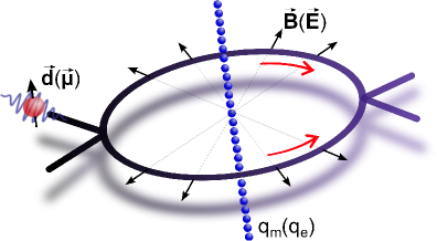
Figure 1: (color online). Connection between the HMW and AC phases by electric-magnetic duality. The HMW phase arises when an electric dipole moment $\mathbf{d}$ propagates in the radial magnetic field created by a line of magnetic monopoles $q_{m}$ while the AC phase (between parenthesis) appears when a magnetic dipole $\boldsymbol{\mu}$ encircles a line of electric charges $q_{e}$.

An Aharonov-Bohm phase appears when a charged particle encircles an infinite line of magnetic dipoles. By exchanging the roles of the charged particle and of the magnetic dipole, Y. Aharonov and A. Casher AharonovPRL84 predicted in 1984 a topological phase when a magnetic dipole encircles an infinite line of electric charges (see fig. 1). This phase had already been predicted in 1982 by J. Anandan AnandanPRL82 , with no insistence on its topological character. The Aharonov-Casher (AC) phase is given by:

$$\varphi_{AC}=-\frac{1}{\hbar c^{2}}\oint\left[\mathbf{E}\left(\mathbf{r}\right)\times\boldsymbol{\mu}\right]\cdot d\mathbf{r}$$ (2)

where $\boldsymbol{\mu}$ is the magnetic dipole and $\mathbf{E}$ the electric field. As for the AB effect, the nature of the AC effect was widely discussed KleinPhysica86 ; BoyerPRA87 ; AharonovPRA88 ; ReznikPRD89 ; GoldhaberPRL89 ; AnandanPLA89 ; LiangPRL89 ; VaidmanAJP90 ; LiangMPLA90 ; HagenPRL90 ; HagenIJMP91 ; RubioNC91 ; MignaniJPA91 ; GoldhaberPLB91 ; ZeilingerPLA91 ; HePLB91 ; HePLB91Bis ; HolsteinAJP91 ; LiangIJMP92 ; HanPLA92 ; SpavieriEPL92 ; LiangPLA93 ; RamseyPRA93 ; BalatskyPRL93 ; ChoiPRL93 ; ReznikPLB93 ; SpavieriNC94 ; LeePLA94 ; PeshkinPRL95 ; AlJaberNC95 ; LeeMPL96 ; FreemanEJP97 ; PeshkinFoP99 ; AharonovPRL00 ; SpavieriNC00 ; SwanssonJPA01 ; BoyerFoP02 ; HyllusPRL02 ; AharonovPRL02 ; DulatPRL12 . In the non-relativistic limit (an excellent approximation for matter wave interferometers if we except electron interferometers), we can demonstrate eq. 2, starting from the Lagrangian of a particle of mass $m$ and velocity $\mathbf{v}=\mathbf{\dot{r}}$ carrying a magnetic dipole $\boldsymbol{\mu}$ in an electric field AharonovPRL84 :

$$L=\frac{1}{2}m\mathbf{v}^{2}-\frac{1}{c^{2}}\mathbf{v}\cdot\left(\mathbf{E}\left(\mathbf{r}\right)\times\boldsymbol{\mu}\right)$$ (3)

The particle acceleration $\mathbf{\dot{v}}$ is given by Lagrange equation AharonovPRA88 :

$$m\mathbf{\dot{v}}=\left(\boldsymbol{\mu}\cdot\nabla\right)\left(\frac{\mathbf{E}\left(\mathbf{r}\right)\times\mathbf{v}}{c^{2}}\right)$$ (4)

In the configuration of ref. AharonovPRL84 , with a straight homogeneously charged line, the right-hand term of eq. 4 vanishes: no force acts on the particle.

A heuristic point of view introduced by A.G. Klein KleinPhysica86 relates the AC phase results to the interaction of the magnetic moment $\boldsymbol{\mu}$ with the motional magnetic field $\mathbf{B}_{mot}\approx-\left(\mathbf{v}\times\mathbf{E}\right)/c^{2}$ experienced by the particle in its rest frame, and calculated at first order in $v/c$. Substituting $d\mathbf{r}=\mathbf{v}dt$ into eq. 2 yields $\varphi_{AC}=\oint\left(\boldsymbol{\mu}\cdot\mathbf{B}_{mot}\right)dt/\hbar$, a result identical to the phase due to the magnetic dipole interaction $-\boldsymbol{\mu}\cdot\mathbf{B}_{mot}$. Eq. (3) reads $L=m\mathbf{v}^{2}/2+L_{AC}$, where $L_{AC}=\boldsymbol{\mu}\cdot\mathbf{B}_{mot}$ is the additional term due to the electric field. Although $-L_{AC}$ looks like a potential energy, it is not a potential energy for the motion of the particle, because $m\mathbf{\dot{v}}$ given by equation (4) is not equal to $\nabla\left(\boldsymbol{\mu}\cdot\mathbf{B}_{mot}\right)$. Indeed, the use of Newton’s equation with the force $\nabla\left(\boldsymbol{\mu}\cdot\mathbf{B}_{mot}\right)$ leads to incorrect results with regards to the topological nature of the AC phase BoyerPRA87 ; AharonovPRA88 ; GoldhaberPRL89 .

To deduce the AC phase from the Lagrangian (eq. (3)), we apply Feynman’s path integral FeynmanRMP48 to matter-wave interferometry CohenJDP94 . At first-order of perturbation theory, the phase $\varphi_{AC}$ is given by the classical action calculated along the unperturbed interferometer arms:

$$\varphi_{AC}=\frac{1}{\hbar}\oint\mathbf{p}_{AC}\cdot d\mathbf{r}$$ (5)

where $\mathbf{p}_{AC}=\partial L_{AC}/\partial\mathbf{v}=-\mathbf{E}\left(\mathbf{r}\right)\times\boldsymbol{\mu}/c^{2}$ is the modification of the particle momentum by the electric field.

II.3 Detection of the AC phase

The AC phase was first detected by A. Cimmino et al. CimminoPRL89 ; KaiserPhysicaB88 using a neutron interferometer. The neutron magnetic dipole is small and the AC phase was only $1.50$ mrad for $E\approx 30$ MV/m. Because of limited neutron flux, $35$ days were needed to get one measurement. Further tests (proportionality to the electric field, independence with neutron velocity) were not feasible.

A noticeable difference between the AB and AC phases is that the particle must propagate in an electric field to get a non-zero AC phase. This circumstance gives more freedom in the field configurations and, in particular, the electric charge between the interferometer arms may vanish AnandanPLA89 ; CasellaPRL90 . K. Sangster et al. SangsterPRL93 ; SangsterPRA95 used this possibility to perform a measurement of the AC phase with a Ramsey interferometer RamseyPR50 : a molecular beam, prepared in a coherent superposition of states with opposite magnetic dipoles, propagates in an electric field perpendicular to the beam velocity. The AC phase shift has opposite values for these two states and the resulting phase difference is directly detected on the fringe signal. The AC phase, measured with a few percent error bar, was found in agreement with theory SangsterPRL93 ; SangsterPRA95 ; its proportionality to the electric field and its velocity independence were both successfully tested. Several other measurements of the AC phase have been performed, always with Ramsey interferometers ZeiskeAPB95 ; GorlitzPRA95 ; YanagimachiPRA02 . The AC effect has also been observed in interference of vortices in a Josephson-junction array ElionPRL93 .

II.4 The He-McKellar-Wilkens phase

In 1993, X.G. He and B.H.J. McKellar HePRA93 applied Maxwell duality to the AC phase, thus predicting a new topological phase when a particle with an electric dipole $\mathbf{d}$ encircles an infinite line of magnetic monopoles (see fig. 1). Because of the hypothetical character of magnetic monopoles milton06 , this paper did not suggest any test but M. Wilkens WilkensPRL94 proposed an experiment, with an electric dipole produced by the polarization of an atom or a molecule, interacting with a magnetic field $\mathbf{B}$ guided by ferromagnetic materials. The general expression of the HMW phase is:

$$\varphi_{HMW}=\frac{1}{\hbar}\oint\left(\mathbf{B}\left(\mathbf{r}\right)\times\mathbf{d}\right)\cdot d\mathbf{r}$$ (6)

Fig. 1 is inspired by the work of J.P. Dowling et al. DowlingPRL99 who gave an overview of the electromagnetic topological phases. Maxwell duality applied to the AB phase leads to a fourth topological phase for a magnetic monopole encircling a line of electric dipoles: this phase will remain hypothetical as long as magnetic monopoles.

The AB phase involves a particle carrying an electric charge and the AC and HMW phases involve particles carrying magnetic and electric dipoles: it is natural to predict topological phases for particles carrying higher-order electromagnetic multipoles, in interaction with electric or magnetic fields of the convenient symmetry. A calculation for the case of electric or magnetic quadrupoles was made by C.-C. Chen ChenPRA95 who states that, with quadrupoles of the order of one atomic unit, the detection of these new topological phases ”would require an unrealistically huge electromagnetic field”. As a consequence, these higher-order phases appear to be out of reach and the HMW phase was the last undetected topological phase of electromagnetic origin.

II.5 Some properties of the HMW effect and the associated particle dynamics

In complete analogy with the AC effect, the HMW effect can be interpreted as due to the interaction of the electric dipole $\mathbf{d}$ with the motional electric field $\mathbf{E}_{mot}\approx\mathbf{v}\times\mathbf{B}$, at the lowest order in $v/c$. Equation (6) can be rewritten:

$$\varphi_{HMW}=\frac{1}{\hbar}\oint\mathbf{d}\cdot\mathbf{E}_{mot}dt$$ (7)

A remark first done by Wei et al. WeiPRL95 suggests a strong link between the AB and the HMW phases. Consider the particular field configuration illustrated by fig. 2, where the electric dipole which undergoes the HMW phase shift is induced by an external electric field (more details are given in part III.1). If the dipole is described by two particles with charges $\pm q$ at positions $\mathbf{r}_{\pm}$, with $\mathbf{d}=q\left(\mathbf{r}_{+}-\mathbf{r}_{-}\right)$, the HMW phase is equal to the algebraic sum of the AB phases for the two particles.

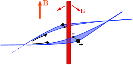
Figure 2: (color online). Connection between the HMW and the AB phases following Wei et al. WeiPRL95 . The interferometer arms (blue full lines) encircle an infinite charged wire (red vertical cylinder) which produces a radial electric field $\mathbf{E}$ and induces an electric dipole $\mathbf{d}$ represented by a positive charge ($+$, large bullet) and a negative charge ($-$, small bullet). Each charge undergoes the AB effect in the uniform magnetic field $\mathbf{B}$. The HMW phase is equal to the sum of the two AB phases and it is proportional to the magnetic flux through the (blue) shaded surface.

The HMW effect and its connection with the AB and AC effects has been the subject of many theoretical works LiuCPL95 ; YiPRB95 ; SpavieriNC96 ; HagenPRL96 ; WeiPRL96 ; SpavieriPRL98 ; WilkensPRL98 ; LeonhardtEPL98 ; AudretschPLA98 ; AudretschPRA99 ; LeonhardtPLA99 ; AudretschPLA99 ; SpavieriPRA99 ; SpavieriPRL99 ; TkachukPRA00 ; AnandanPRL00 ; LeePRA00 ; LeePRA01 ; SpavieriPLA03 ; FurtadoPRA04 ; IvezicPRL07 . Let us summarize the main results concerning the dynamics of an electric dipole in a magnetic field. The electric dipole moment $\mathbf{d}=q\mathbf{r}_{0}$ is described by two charges with $\mathbf{r}_{0}=\mathbf{r}_{+}-\mathbf{r}_{-}$ and its internal dynamics is described by an interaction energy $U\left(r_{0}\right)$, function of the distance $r_{0}$ between the charges. The compound particle (mass $M$, center of mass $\mathbf{r}$, velocity $\mathbf{v}=\dot{\mathbf{r}}$) interacts with an external electromagnetic field described by its potential $\left(\mathbf{A}\left(\mathbf{r},t\right),V\left(\mathbf{r},t\right)\right)$, with the electric field $\mathbf{E}\left(\mathbf{r},t\right)=-\nabla V-\partial\mathbf{A}/\partial t$ and the magnetic field $\mathbf{B}\left(\mathbf{r},t\right)=\nabla\times\mathbf{A}$. The standard Lagrangian for the system, expressed in the dipole approximation, is SpavieriPRA99 :

$$L = \frac{1}{2}M{\dot{\mathbf{r}}}^{2}+\frac{1}{2}\mu{\dot{\mathbf{r}}_{0}}^{2}+\dot{\mathbf{r}}\cdot\left[\left(\mathbf{d}\cdot\nabla\right)\mathbf{A}\left(\mathbf{r},t\right)\right]$$

$$\quad+\dot{\mathbf{d}}\cdot\mathbf{A}\left(\mathbf{r},t\right)-\left(\mathbf{d}\cdot\nabla\right)V\left(\mathbf{r},t\right)-U\left(r_{0}\right)$$

where $M$ is the total mass of the compound particle and $\mu$ is the reduced mass of the two particles. Expanding the total derivative $d/dt=\partial/\partial t+\left({\dot{\mathbf{r}}}\cdot\nabla\right)$, it can be rewritten:

$$L = \frac{1}{2}M{\dot{\mathbf{r}}}^{2}+\frac{1}{2}\mu{\dot{\mathbf{r}}_{0}}^{2}+L_{W}-U\left(r_{0}\right)+\frac{d}{dt}\left(\mathbf{d}\cdot\mathbf{A}\right)$$

$$\text{with: }L_{W}=\mathbf{d}\cdot\left(\mathbf{E}+\mathbf{v}\times\mathbf{B}\right)$$

$L_{W}$ is the term introduced by M. Wilkens WilkensPRL94 to describe the interaction of the dipole with the field. In his calculation, the total derivative term $d\left(\mathbf{d}\cdot\mathbf{A}\right)/dt$ was omitted. Because this total derivative is a single valued function of the dynamical variables and of time, the standard Lagrangian and the Lagrangian proposed by Wilkens are strictly equivalent SpavieriPRL98 ; WilkensPRL98 . With the Lagrangian used by Wilkens, the canonical momenta are given by:

$$\mathbf{p} = \frac{\partial L}{\partial\dot{\mathbf{r}}}=M\mathbf{v}+\mathbf{B}\times\mathbf{d}$$ (10)

$$\mathbf{p}_{0} = \frac{\partial L}{\partial{\dot{\mathbf{r}}}_{0}}=\mu{\dot{\mathbf{r}}}_{0}$$ (11)

As for the AC effect, the extra-contribution $\mathbf{p}_{HMW}=\mathbf{B}\times\mathbf{d}$ to the momentum $\mathbf{p}$ yields the HMW phase:

$$\varphi_{HMW}=\frac{1}{\hbar}\oint\mathbf{p}_{HMW}\cdot d\mathbf{r}$$ (12)

The Lagrange equations yield the dynamics of the particle in the laboratory frame and its internal dynamics:

$$M\ddot{\mathbf{r}} = \dot{\mathbf{d}}\times\mathbf{B}+\left(\mathbf{d}\cdot\nabla\right)\left[\mathbf{E}+\mathbf{v}\times\mathbf{B}\right]$$ (13)

$$\mu\ddot{\mathbf{r}}_{0} = q\left(\mathbf{E}+\mathbf{v}\times\mathbf{B}\right)-\frac{\partial U}{\partial\mathbf{r}_{0}}$$ (14)

In the original configuration with an infinite line of magnetic monopoles line (see Fig. 1), the force on the particle vanishes. Here is a brief summary of the explanation given by M. Wilkens WilkensPRL94 . The dipole dynamics is limited to rotation, with the dipole initially parallel to the line of monopoles, while the particle propagates in a plane perpendicular to this line. The torque exerted on the dipole, $\mathbf{d}\times\left(\mathbf{E}+\mathbf{v}\times\mathbf{B}\right)$ vanishes and we may drop the term $\dot{\mathbf{d}}\times\mathbf{B}$ from Eq. ((13)). If the fields $\mathbf{E}$ and $\mathbf{B}$ are invariant by a translation along the direction of the dipole, the force vanishes.

A closer look is needed in the case of an induced dipole. In this case, it is a good approximation to consider that the variations of the external fields in the frame moving with the atom are infinitely slow and that the dynamics of $\mathbf{r_{0}}$ is adiabatic, so that the atom exhibits the dipole $\mathbf{d}=4\pi\varepsilon_{0}\alpha\left(\mathbf{E}+\mathbf{v}\times\mathbf{B}\right)$, where $\alpha$ is the polarizability. With this approximation, one obtains the Lagrangian proposed by Wei et al WeiPRL95 :

$$L=\frac{1}{2}M{\dot{\mathbf{r}}}^{2}+2\pi\varepsilon_{0}\alpha{\left(\mathbf{E}+\mathbf{v}\times\mathbf{B}\right)}^{2}$$ (15)

From this Lagrangian, it is easy to deduce the force on the atom and we consider here only three terms which involve the presence of $\mathbf{E}$ and $\mathbf{B}$ simultaneously:

$$\mathbf{F}_{1} = 4\pi\varepsilon_{0}\alpha\left(\mathbf{\dot{E}}\times\mathbf{B}\right)$$

$$\mathbf{F}_{2} = 4\pi\varepsilon_{0}\alpha\left(\mathbf{v}\times\mathbf{B}\right)\cdot\nabla\mathbf{E}$$

$$\mathbf{F}_{3} = 4\pi\varepsilon_{0}\alpha\mathbf{E}\cdot\nabla\left(\mathbf{v}\times\mathbf{B}\right)$$ (16)

We assume that both fields are static i.e. $\partial\mathbf{E}/\partial t=\mathbf{0}=\partial\mathbf{B}/\partial t$. $\mathbf{F}_{1}$ is non-zero in the regions where the electric field is inhomogeneous because, in the atom frame, $\mathbf{\dot{E}}=\left(\mathbf{v}\cdot\nabla\right)\mathbf{E}$. When the electric field varies, the dipole varies too, which induces a current, and $\mathbf{F}_{1}$ is the associated Lorentz force. If we take the $\mathbf{z}$ axis along the velocity $\mathbf{v}=v\mathbf{z}$ and the $\mathbf{y}$ axis along the magnetic field $\mathbf{B}=B\mathbf{y}$, we are interested only in the $z$-components of the forces because they are the only ones which can change the velocity:

$$F_{1,z} = 4\pi\varepsilon_{0}\alpha vB\frac{\partial E_{x}}{\partial z}$$

$$F_{2,z} = -4\pi\varepsilon_{0}\alpha vB\frac{\partial E_{z}}{\partial x}$$

$$F_{3,z} = 0$$ (17)

As $\nabla\times\mathbf{E}=-\partial\mathbf{B}/\partial t=0$, then $\partial E_{x}/\partial z=\partial E_{z}/\partial x$ and $F_{1,z}+F_{2,z}=0$: in the Wilkens-Wei configuration WilkensPRL94 ; WeiPRL95 , the HMW phase is a topological phase.

III Toward a detection of the HMW phase

In this section, we describe various proposals for the detection of the HMW phase, and we explain the choices we have made for our experiment.

III.1 Possible detection schemes

The detection of the HMW phase is difficult for two reasons: we need a particle with an electric dipole and we must replace the radial magnetic field of a line of magnetic monopoles by some other field configuration. Here are the experimental schemes proposed for this detection:

• M. Wilkens WilkensPRL94 proposed to polarize atoms (or molecules) by an electric field $\mathbf{E}$, thus inducing a dipole $\mathbf{d}=4\pi\varepsilon_{0}\alpha\mathbf{E}$, and to apply different magnetic fields on the two interferometer arms thanks to a pierced sheet of ferromagnetic material. The use of such a sheet appears to be very difficult because of the small distance between interferometer arms and of the associated perturbation of the electric field. However, this proposal opened the way toward experiments.

• H. Wei et al. WeiPRL95 proposed to introduce a charged wire between the arms of an atom interferometer, thus inducing opposite dipoles on the two interferometer arms, and to use a common homogeneous magnetic field to induce the HMW phase. Figures 2 and 3 illustrates this scheme, and figure 3 depicts our own configuration which is directly inspired by this proposal.

• H. Wei et al. WeiPRL95 also predicted a persistent current in a polarizable superfluid (see also YiPRB95 ). Following this idea, Y. Sato and R. Packard SatoJOP09 have proposed to detect the HMW phase with a superfluid helium interferometer.

It would be very convenient to use a Ramsey interferometer to detect the HMW phase, as done for most of the AC phase measurements SangsterPRL93 ; SangsterPRA95 ; ZeiskeAPB95 ; GorlitzPRA95 ; YanagimachiPRA02 . Such an interferometer requires a coherent superposition of states with opposite electric dipole moments SpavieriPRL99 ; DowlingPRL99 , which seems feasible with molecules or with Rydberg atoms, because they have quasi-degenerate states of opposite parity DowlingPRL99 , but not with ground state atoms. As a consequence, Ramsey interferometry with ground state atoms cannot be used for the detection of the HMW phase. Instead, the HMW phase will be given by the difference of successive phase measurements, a technique more sensitive to systematic effects than Ramsey interferometry.

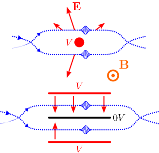
Figure 3: (color online). Geometry of the electric field for the detection of the HMW phase, following the proposal of Wei et al. WeiPRL95 . The atom (blue dots) propagates in the interferometer plane, with the homogeneous magnetic field $\mathbf{B}$ perpendicular to this plane. The conductors are shown with their potential (red or black if grounded) and the electric field vector $\mathbf{E}\left(\mathbf{r}\right)$ is represented by red arrows for some sample positions along the interferometer arms. Upper panel (similar to fig. 2): the original proposal with a charged wire which produces a strongly inhomogeneous electric field. Lower panel: our geometry with homogeneous electric fields produced by plane capacitors.

III.2 Principle of our experiment

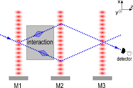
Figure 4: (color online). Schematic top-view of our atom interferometer: the HMW interaction region is placed just before the second laser standing wave, at the place where the arm separation is largest. It is thus possible to introduce a septum between the two interferometer arms without any perturbation of the interferometer signal.

To detect the HMW phase, we have built an experiment LepoutrePhD ; LepoutrePRL12 with our atom interferometer MiffreEPJD05 ; MiffrePhD (see fig. 4). A highly collimated supersonic beam of lithium seeded in argon, with a mean lithium velocity $v_{m}\approx 1065$ m/s, crosses three quasi-resonant laser standing waves which diffract the atoms in the Bragg regime. With first order Bragg diffraction which produces only two diffracted beams (orders $p=0$ and either $p=+1$ or $p=-1$), we get in this way an almost perfect Mach-Zehnder interferometer. A slit selects one of the two output beams carrying complementary interference signals and the intensity $I$ of this beam, measured by a surface ionization detector, is the output signal of the interferometer:

$$I=I_{0}\left[1+\mathcal{V}\cos\left(\varphi_{d}+\varphi_{p}\right)\right]$$ (18)

$I_{0}$ is the mean intensity, $\mathcal{V}$ is the fringe visibility and $\varphi_{p}$ is the phase due to various perturbations. The phase $\varphi_{d}$, due to laser diffraction, is a function of the positions $x_{i}$ of the three standing wave mirrors M_i: $\varphi_{d}=2k_{L}(x_{1}-2x_{2}+x_{3})$, where $k_{L}$ is the laser wavevector. The choice of the laser frequency, very close to the first resonance transition of lithium MiffreEPJD05 , and the natural abundance of ⁷Li ($92.5$%) make that the signal is purely due to this isotope MiffreEPJD05 ; JacqueyEPL07 .

To observe a non-zero HMW phase, the atom must propagate in crossed electric and magnetic fields transverse to its velocity and the fields on the two interferometer arms must be different. Near the second laser standing wave, the two arms are separated by a distance close to $100$ $\mu$m, sufficient to insert a septum between the two arms. A septum can be used to produce different magnetic fields by circulating a current in the septum SchmiedmayerJPII94 or different electric fields with two capacitors sharing the septum as a common electrode EkstromPRA95 . The difference of magnetic fields achieved in ref. SchmiedmayerJPII94 was quite small, near $10^{-5}$ T, limited by the current in the septum, while the second arrangement EkstromPRA95 has produced intense electric fields, of the order of $1$ MV/m. We have chosen the second arrangement with opposite electric fields on the two interferometer arms and a common magnetic field: in addition to the HMW phase, this arrangement produces several other phases discussed in sections V and VI. This setup is very close to the idea of Wei et al. WeiPRL95 but the charged wire is replaced by a septum, which improves considerably the electric field homogeneity.

IV Effect of a dispersion of the phase on the interferometer signal

Any dispersion of the phase $\varphi=\varphi_{d}+\varphi_{p}$ reduces the fringe visibility ${\mathcal{V}}$ and a good visibility is necessary for accurate phase measurements. In this part, we study the origins of phase dispersions and the associated systematic effects.

IV.1 Origins of phase dispersion

The interferometer phase is dispersed because of its dependence with the atom velocity, with the atom trajectory and with the atom internal state.

The diffraction phase $\varphi_{d}$ is independent of the atom velocity $v$ but the perturbation phase $\varphi_{p}$ is a priori a function of $v$. A dynamic phase due to a perturbation applied to one arm is proportional to $1/v$. If the same perturbation is applied to both arms, the phase shift vanishes if the perturbation is homogeneous and is proportional to $1/v^{2}$ in the presence of a perturbation gradient, with an extra $1/v$-factor due to the distance between the interferometer arms which is approximately proportional to $1/v$. The topological AC and HMW phases are independent of the velocity. Finally, inertial phase shifts are proportional to $1/v$ (Sagnac effect) and to $1/v^{2}$ (homogeneous gravitational field): in our experiment, there is a small Sagnac phase due to Earth rotation JacqueyPRA08 but the phase due to the gravitational field vanishes because the interferometer is an horizontal plane.

In our experiment, the magnetic field is slightly inhomogeneous and the electric fields have slightly different modulus on the two interferometer arms. Atom diffraction is in the horizontal plane, which means that the interferometer signal is sensitive to the difference of the propagation phases on the two arms at the same altitude $y$. The resulting phase shifts are functions of the $y$-coordinate because of the spatial dependence of the fields.

The diffraction phase shift $\varphi_{d}$ is also a function of the $y$-coordinate, if the laser standing wave mirrors M_i are not perfectly aligned (for an analysis, see ref. ChampenoisEPJD99 ; ChampenoisPhD ). The final alignment of these mirrors is done by optimizing the fringe visibility MiffreEPJD05 and this procedure is not sensitive to a small residual $y$-dependence of $\varphi_{d}$.

The Zeeman phase is a function of the hyperfine-Zeeman $F,m_{F}$ sublevel; this phase, which may be large, varies rapidly with $F,m_{F}$ (see section VI). The interferometer signal is the sum of the contributions of these 8 sublevels: in the absence of optical pumping, the sublevels are equally populated in the incident atomic beam, but the interferometer transmission is a function of the hyperfine level $F$. As a consequence, the 8 sublevels may have different populations in the detected signal: this question is discussed in Appendix A.

IV.2 Effect of the velocity dependence of the phase-shifts

The normalized velocity distribution of a supersonic beam is given by:

$$P(v)=\frac{S_{\|}}{v_{m}\sqrt{\pi}}\exp\left[-\left(\frac{\left(v-v_{m}\right)S_{\|}}{v_{m}}\right)^{2}\right]$$ (19)

$v_{m}$ is the mean velocity, $S_{\|}$ is the parallel speed ratio. A $v^{3}$ pre-factor, usually included HaberlandRSI85 , has been omitted for two reasons: - when $S_{\|}$ is large, this pre-factor has small effects; - because of the use of Bragg diffraction, the interferometer transmission is a function of the velocity and this effect modifies the velocity distribution. We consider a perturbation phase $\varphi_{p}(v)\propto 1/v^{n}$ so that we can write $\varphi_{p}(v)=\varphi_{p}(v_{m})(v_{m}/v)^{n}$. The interferometer signal is the velocity-average of eq. (18):

$$I=I_{0}\int dvP(v)\left[1+{\mathcal{V}}\cos\left(\varphi_{d}+\varphi_{p}(v_{m})\left(\frac{v_{m}}{v}\right)^{n}\right)\right]$$ (20)

If the ratio $\varphi_{p}(v_{m})/S_{\|}$ is not too large, it is a good approximation to expand $v_{m}/v$ up to the second order in powers of $(v-v_{m})/v_{m}$ and the integral can be calculated analytically MiffreEPJD06 ; MiffrePhD . The phase shift differs from $\varphi_{p}(v_{m})$ by a term linear in $\varphi_{p}(v_{m})/S_{\|}^{2}$ because of the non-linear dependence of $\varphi_{p}$ with $v$ and the visibility decreases rapidly when $\varphi_{p}(v_{m})\approx S_{\|}/n$, with a quasi-Gaussian dependence.

IV.3 Calculation of the effect of a narrow distribution of phase shift

Eq. (20) uses analytical expressions of $\varphi(v)$ and of $P(v)$. For other types of phase dispersion, this information is not generally available. For instance, for the dependence of the phase with the atom trajectory, we may assume that the phase is a function $\varphi(y)$ of a continuous variable $y$ with a normalized probability $P(y)$ and we must average eq. (18):

$$\left<I\right>=I_{0}\int dyP(y)\left[1+{\mathcal{V}}\cos\left(\varphi(y)\right)\right]$$ (21)

$\left<...\right>$ denotes the average over $y$ with the weight $P(y)$. We assume that the visibility ${\mathcal{V}}$ is independent of $y$ because the fringe visibility has a very low sensitivity to the diffraction amplitudes MiffreEPJD05 . We introduce:

$$\left<\varphi\right>=\int dyP(y)\varphi(y)$$ (22)

$$\delta\varphi=\varphi(y)-\left<\varphi\right>$$

Obviously $\left<\delta\varphi\right>=0$. Assuming that $\delta\varphi$ is small, we expand $\sin\left(\delta\varphi\right)$ and $\cos\left(\delta\varphi\right)$ up to third order in $\delta\varphi$ (these expansions are of reasonable accuracy even if $\left|\delta\varphi\right|\approx 1$ rad). Once averaged over $y$, eq. (21) is similar to eq. (18) with a modified visibility $\mathcal{V}_{m}$ and a modified phase $\varphi_{m}$:

$$\mathcal{V}_{m}/\mathcal{V}_{0} = 1-\left<\left(\delta\varphi\right)^{2}/2\right>$$

$$\varphi_{m} = \left<\varphi\right>-\left<\left(\delta\varphi\right)^{3}/6\right>$$ (23)

The reduced visibility $\mathcal{V}_{r}=\mathcal{V}_{m}/\mathcal{V}_{0}$ carries interesting information when two perturbations $a$ and $b$ inducing the phases $\varphi_{a}$ and $\varphi_{b}$ are simultaneously applied:

$$\mathcal{V}_{r,a+b}=\frac{\mathcal{V}_{m,a+b}}{\mathcal{V}_{0}} = 1-\frac{\left<\left(\delta\varphi_{a}+\delta\varphi_{b}\right)^{2}/2\right>}{2}$$ (24)

$$\approx \mathcal{V}_{r,a}\mathcal{V}_{r,b}\left[1-\left<\delta\varphi_{a}\delta\varphi_{b}\right>\right]$$

By measuring three reduced visibility $\mathcal{V}_{r,a}$, $\mathcal{V}_{r,b}$ and $\mathcal{V}_{r,a+b}$, we have access to the correlation $\left<\delta\varphi_{a}\delta\varphi_{b}\right>$ of the dispersions of the two phases. The phase shift $\varphi_{m}$ due to the perturbation is not equal to the mean phase $\left<\varphi\right>$ because, even if, by definition, $\left<\delta\varphi\right>=0$, $\left<\left(\delta\varphi\right)^{3}\right>$ is usually not equal to $0$. Moreover, if two perturbations $a$ and $b$ are simultaneously applied, the phase shifts are not additive, because of the cross-terms $\left<\delta\varphi_{a}^{2}\delta\varphi_{b}\right>$ and $\left<\delta\varphi_{a}\delta\varphi_{b}^{2}\right>$.

IV.4 Discrete average over Zeeman-hyperfine sublevels

The signal is given by:

$$I = I_{0}\sum_{j}P_{j}\left[1+\mathcal{V}_{j}\cos\left(\left<\varphi_{j}\right>\right)\right]$$ (25)

where the signal due to the sublevel $j$ is characterized by a normalized population $P_{j}$ ($\sum_{j}P_{j}=1$), a visibility $\mathcal{V}_{j}$ and a phase $\varphi_{j}$. The visibility $\mathcal{V}_{j}$ varies with the sublevel because the reduction of visibility given by eq. (IV.3) is a function of the sublevel. The $-\left<\left(\delta\varphi_{j}\right)^{3}/6\right>$ term, omitted in eq. (25), will be taken into account in the complete calculation. For the contribution of sublevel $j$ to the signal, we define a complex fringe visibility $\underline{\mathcal{V}}_{j}$ given by:

$$\underline{\mathcal{V}}_{j}=\mathcal{V}_{j}\exp\left(i\left<\varphi_{j}\right>\right)$$ (26)

The complex visibility for the total signal is given by:

$$\underline{\mathcal{V}}= \sum_{j}P_{j}\underline{\mathcal{V}}_{j}$$ (27)

This is a Fresnel construction from which we deduce the modified fringe visibility $\mathcal{V}_{m}$ and phase $\varphi_{m}$:

$$\mathcal{V}_{m} = \sqrt{\left[\sum P_{j}\mathcal{V}_{j}\cos\left<\varphi_{j}\right>\right]^{2}+\left[\sum P_{j}\mathcal{V}_{j}\sin\left<\varphi_{j}\right>\right]^{2}}$$

$$\tan\varphi_{m} = \left(\sum P_{j}\mathcal{V}_{j}\sin\left<\varphi_{j}\right>\right)/\left(\sum P_{j}\mathcal{V}_{j}\cos\left<\varphi_{j}\right>\right)$$ (28)

When the phases $\left<\varphi_{j}\right>$ are very close to their mean, the resulting phase $\varphi_{m}$ is their weighted average, but the weights are the products $P_{j}\mathcal{V}_{j}$ and not the populations $P_{j}$. This result has an important consequence: when a perturbation modifies the visibility $\mathcal{V}_{j}$, the modified phase $\varphi_{m}$ is not a simple average of $\left<\varphi_{j}\right>$. In this case too, even without the non-linear term $\left<\delta\varphi^{3}\right>/6$, the phase shifts resulting from two perturbations are not additive, because the weights $P_{j}\mathcal{V}_{j}$ are different in the three cases : application of perturbation $a$, application of perturbation $b$ and simultaneous application of both perturbations.

V Effects of the electric field on the interferometer signals

An electric field induces a large phase due to Stark effect and a small one due to Aharonov-Casher effect AharonovPRL84 . Because of its dependence on the magnetic dipole moment, the AC phase appears as a modification of the Zeeman effect and we will discuss it after the Zeeman phase in section VII.

V.1 Effective Stark Hamiltonian

If we neglect hyperfine structure, an electric field $\mathbf{E}$ induces only a global displacement of lithium ²S_1/2 ground state described by the Stark Hamiltonian $H_{S}$ :

$$H_{S}=-2\pi\varepsilon_{0}\alpha\mathbf{E}^{2}$$ (29)

$\alpha$ is the electric polarizability, $\alpha=(24.34\pm 0.16)\times 10^{-30}$ m³ MiffreEPJD06 ; JacqueyPRA08 . Theoretical values PuchalskiPRA12 are considerably more accurate and in good agrement with this experimental value. For our largest field $E_{max}\approx 0.8$ MV/m, the Stark energy is $E_{S}\approx 10^{-27}$ J while the atom kinetic energy is $K=mv_{m}^{2}/2\approx 7\times 10^{-21}$ J. With $E_{S}/K$ smaller than $2\times 10^{-7}$, a first order perturbation calculation of the Stark phase is fully justified:

$$\varphi_{S}=2\pi\varepsilon_{0}\alpha\oint\mathbf{E}^{2}dt/\hbar$$ (30)

If the field $E_{max}\approx 0.8$ MV/m was applied on one interferometer arm only, the Stark phase would be large, $\varphi_{S}\approx 300$ rad. In the experiments devoted to the detection of the HMW phase, opposite electric fields are applied on the two interferometer arms, resulting in a very small detected Stark phase shift.

Because of its $3/2$ nuclear spin, ⁷Li has $8$ hyperfine-Zeeman sublevels. The Stark shift is only approximately independent of the sublevel but this dependence is very weak. This question is very important for atomic clocks and it has been studied theoretically by Sandars SandarsPPS67 and Ulzega et al. UlzegaEPL06 : the results are in good agreement with experiments for the cesium clock SimonPRA98 ; OspelkausPRA03 . For ⁷Li, only the energy shift difference $\Delta\textrm{E}_{S}$ of the $F=1$, $m_{F}=0$ and $F=2$, $m_{F}=0$ sublevels has been measured MowatPRA72 , $\Delta\textrm{E}_{S}/h=-0.061(2)\times 10^{-10}E^{2}$ Hz with $E$ in V/m. This measurement is in good agreement with theoretical values KaldorJPB73 ; PuchalskiPRA12 . The ratio of this differential shift to the mean energy shift is $\Delta\textrm{E}_{S}/\textrm{E}_{S}\approx 3\times 10^{-6}$ and we may deduce that the $F,m_{F}$-dependence of the Stark phase is negligible in our experiment.

V.2 Stark phase-shift of an ideal experiment

We first assume defect-free capacitors, with plane parallel electrodes. We use the same notations as in ref. MiffreEPJD06 : electrode spacing $h_{i}$ and length between the guard electrodes $2a_{i}$. The electric field $\mathbf{E}_{i}(z)$ is easily calculated MiffreEPJD06 and the Stark phase shift $\varphi_{S,i}$ for an atom in the interferometer arm $i$ is given by:

$$\varphi_{S,i} = \frac{2\pi\epsilon_{0}\alpha}{\hbar v}\int\mathbf{E}_{i}^{2}(z)dz$$ (31)

$$= \frac{2\pi\epsilon_{0}\alpha}{\hbar v}\frac{V_{i}^{2}}{h_{i}^{2}}L_{i}$$

where $L_{i}=\left[2a_{i}-(2h_{i}/\pi)\right]$ is the effective length of capacitor $i$ and $V_{i}$ the potential difference across the capacitor. The small correction MiffreEPJD06 due to the fact that the atom passes at a distance ca. $40$ $\mu$m of the septum, is negligible. The Stark phase shift $\varphi_{S}$ is the difference of these two phase shifts:

$$\varphi_{S} = \varphi_{S,l}-\varphi_{S,u}=\frac{2\pi\epsilon_{0}\alpha}{\hbar v}\left[\frac{V_{l}^{2}}{h_{l}^{2}}L_{l}-\frac{V_{u}^{2}}{h_{u}^{2}}L_{u}\right]$$ (32)

where $l$ ($u$) refers to the upper (lower) arm of the interferometer as schemed in fig. 4. By tuning the voltage ratio $V_{u}/V_{l}$, we can cancel $\varphi_{S}$ for all atom velocities.

V.3 Taking into account capacitor defects

The two capacitors present geometrical defects: the electrodes and the septum are not perfectly plane and parallel and the design of the guard electrodes is imperfect. We describe these defects by assuming that the spacing $h_{i}(y,z)$ of capacitor $i$ is a slowly varying function of $y$ and $z$ and that the length $L_{i}(y)$ between guard electrodes is a slowly varying function of $y$. Finally, the voltage across the capacitor $i$ is the sum of the applied voltage $V_{i}$ and of contact potentials $V_{c,i}(y,z)$ which is the difference of the work functions of the two electrodes ($V_{c,i}(y,z)$ is of the order of $100$ mV). An exact calculation of the field would be complicated and we assume that the local field $E_{i}(y,z)$ is the field of a perfect plane capacitor of spacing $h_{i}(y,z)$:

$$E_{i}(y,z) = \frac{V_{i}+V_{c,i}(y,z)}{h_{i}(y,z)}$$ (33)

The phase $\varphi_{S,i}$ is a function of $y$:

$$\varphi_{S,i}(y) = \frac{2\pi\epsilon_{0}\alpha}{\hbar v}\int_{L_{i}(y)}E_{i}^{2}(y,z)dz$$ (34)

In an exact calculation of $E_{i}(y,z)$, the small-scale variations of $h_{i}(y,z)$ and $V_{c,i}(y,z)$ would be washed out because the atoms sample the electric field at a distance ca. $40$ $\mu$m of the septum and only variations with a scale larger than this distance may play a role. We will not try to take this effect into account but most of the rapid variations of the electric field are already washed out in the phase because of the integral appearing in equation (34). The calculation of $\varphi_{S,i}(y)$ is detailed in Appendix B. Because $V_{c,i}(y,z)$ is always much smaller than $V_{i}$, the quadratic term in $V_{c,i}(y,z)$ is negligible and we get $\varphi_{S,i}(y)=\varphi_{S,g,i}(y)+\varphi_{S,c,i}(y)$ with a dominant term $\varphi_{S,g,i}\propto V_{i}^{2}$ and a minor term $\varphi_{S,c,i}(y)\propto V_{i}V_{c,i}(y,z)$. The $y$-variations of $\varphi_{S,g}$ are due to geometrical defects:

$$\varphi_{S,g,i}(y) = \frac{2\pi\epsilon_{0}\alpha}{\hbar v}V_{i}^{2}\int_{L_{i}(y)}\frac{dz}{h_{i}^{2}(y,z)}$$ (35)

while the $y$-variations of $\varphi_{S,c,i}(y)$ are mostly due to contact potentials $V_{c,i}(y,z)$:

$$\varphi_{S,c,i}(y) = \frac{4\pi\epsilon_{0}\alpha}{\hbar v}V_{i}\int_{L_{i}(y)}\frac{V_{c,i}(y,z)dz}{h_{i}^{2}(y,z)}$$ (36)

As in eq. (32), the Stark phase shift is the difference of the phases on the two arms $i=l,u$.

VI Effects of the magnetic field on the interferometer signals

In this section, we recall the hyperfine-Zeeman Hamiltonian and we discuss the Zeeman phase shifts resulting from a gradient of the magnetic field between the two interferometer arms.

VI.1 The hyperfine-Zeeman Hamiltonian

For lithium ground state, the hyperfine-Zeeman Hamiltonian $H_{HFS+Z}$ is given by:

$$H_{HFS+Z}=A\mathbf{I}\cdot\mathbf{S}-g_{S}\mu_{B}\mathbf{S}\cdot\mathbf{B}-g_{I}\mu_{B}\mathbf{I}\cdot\mathbf{B}$$ (37)

$\mathbf{S}$ and $\mathbf{I}$ are the electronic ($S=1/2$) and nuclear ($I=3/2$) spins respectively. The ground state is split in two hyperfine levels $F=1,2$ and 8 $F,m_{F}$ sublevels. The Fermi-contact hyperfine parameter $A$, the electronic Landé factor $g_{S}$ and the nuclear Landé factor $g_{I}$ are very accurately known ArimondoRMP77 ; YanPRL01 .

We have omitted the diamagnetic term $H_{dia}=-\sum_{i}q^{2}(r_{\perp,i}^{2})\mathbf{B}^{2}/8m$, where $r_{\perp,i}$ is the projection of the nucleus-electron vector on a plane perpendicular to $\mathbf{B}$. Using $\sum_{i}<r_{i}^{2}>$ given by ref. YanPRA95 , for our largest field, $B_{max}\approx 1.4\times 10^{-2}$ T, the energy shift is $\Delta E_{dia}\approx 2.4\times 10^{-32}$ J, which is very small and independent of the sublevel. Moreover, as the interferometer signal is sensitive only to the difference of $\Delta E_{dia}$ between the two interferometer arms and as the magnetic field homogeneity is very good, the resulting phase is fully negligible.

The Zeeman energy shifts are always smaller than $\mu_{B}B_{max}\approx 1.3\times 10^{-25}$ J and the ratio of these shifts to the kinetic energy is smaller than $2\times 10^{-5}$, which remains small. The magnetic field extends over $\approx 80$ mm corresponding to an interaction time $t_{int}\approx 75$ $\mu$s. If the magnetic field was applied to one interferometer arm only, a first-order perturbation calculation predicts a maximum phase $\varphi_{Z,max}=\mu_{B}B_{max}t_{int}/\hbar\approx 10^{5}$ rad and the second-order term of the perturbation expansion is of the order of $1$ rad, which is not at all negligible. In our experiment, the field homogeneity is good, $\Delta B/B\approx 10^{-4}$, where $\Delta B$ is the difference of the field on the two interferometer arms: with this field difference, the first order term induces a Zeeman phase shift of the order of $10$ rad at most, while the second order terms compensate each other and their contribution to the Zeeman phase shift is negligible, below $1$ mrad. Finally, hyperfine uncoupling cannot be neglected for our maximum field and the hyperfine Zeeman energies are given by:

$$E(F,m_{F},B) = -\frac{A}{4}-g_{I}\mu_{B}m_{F}B\pm A\sqrt{1+m_{F}X+X^{2}}$$

$$\mbox{with }X = -\frac{\left(g_{S}-g_{I}\right)\mu_{B}B}{2A}$$ (38)

with $X=34.9B$ ($B$ in Tesla) so that for our largest field $X\approx 0.5$. If $X<1$, the $\pm$ sign is associated to the $F=I\pm 1/2$ level. If we forget the small $g_{I}\mu_{B}m_{F}B$ term in eq. (VI.1), there are four pairs of levels with opposite Zeeman energy shifts, the three pairs of levels with the same $m_{F}$ value and the pair $F=2,m_{F}=\pm 2$ and this property will be useful. The variations of $E(F,m_{F},X)$ are plotted in fig. 5. Later, we will use the derivatives of $E(F,m_{F},X)$ with respect to $X$, given by:

$$\frac{\partial E(F,m_{F},B)}{A\partial X} \approx -g_{F}m_{F}\pm\left[1-\frac{m_{F}^{2}}{4}\right]X$$ (39)

$$\pm\frac{3m_{F}}{4}\left[\frac{m_{F}^{2}}{4}-1\right]X^{2}$$

This expansion, limited to the $X^{2}$ terms, is exact for the $F=2,m_{F}=\pm 2$ sublevels. For $\left|X\right|<0.5$, its accuracy is better than $3$% for the $m_{F}=\pm 1$ sublevels, but only $12$% for the $m_{F}=0$ sublevels.

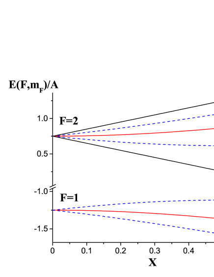
Figure 5: (color online). Hyperfine-Zeeman energies $E(F,m_{F})/A$ plotted as a function of $X=-\left(g_{S}-g_{I}\right)\mu_{B}B/(2A)$. It appears clearly that there are four pair of levels with almost opposite Zeeman energy shifts.

VI.2 Calculation of the Zeeman phases and their effects on the fringe phase and visibility

If the magnetic field never vanishes and if its direction is slowly varying along the atom trajectory, it is a good approximation to assume an adiabatic behavior SchmiedmayerJPII94 ; giltner95 ; JacqueyEPL07 : the projection $m_{F}$ of the total angular momentum $\mathbf{F}$ on an axis parallel to $\mathbf{B}$ is constant and the Zeeman phase is given by:

$$\varphi_{Z}\left(F,m_{F}\right) = -\frac{1}{\hbar v}\oint_{l-u}E(F,m_{F},B)ds$$ (40)

$$\approx \frac{1}{\hbar v}\int\frac{\partial E(F,m_{F},B)}{\partial B}\frac{\partial B}{\partial x}\delta x(z)dz$$

where $\delta x(z)$ is the distance between the interferometer arms at the coordinate $z$ and $B$ is the modulus of the magnetic field. When the magnetic field is produced by a current $I$ circulating in a coil, the dependence with $I$ of the Zeeman phase shifts are complicated. We obtain an approximate analytic expression using the power expansion, eq. (39):

$$\varphi_{Z}\left(F,m_{F}\right) = -g_{F}m_{F}J_{1}\pm\left[1-\frac{m_{F}^{2}}{4}\right]J_{2}$$

$$\pm\frac{3m_{F}}{4}\left[\frac{m_{F}^{2}}{4}-1\right]J_{3}$$

$$J_{1} = \frac{\mu_{B}}{\hbar v}\int\frac{\partial B}{\partial x}\delta x(z)dz$$

$$J_{2} = \frac{\left(g_{S}-g_{I}\right)^{2}\mu_{B}^{2}}{8A\hbar v}\int\frac{\partial(B^{2})}{\partial x}\delta x(z)dz$$

$$J_{3} = \frac{3\left(g_{S}-g_{I}\right)^{3}\mu_{B}^{3}}{128A^{2}\hbar v}\int\frac{\partial(B^{3})}{\partial x}\delta x(z)dz$$ (41)

$J_{k}$ is proportional to ${\left|I\right|}^{k}$ and the Zeeman phase shifts are expressed as third order polynomials of $I$. Moreover, the presence and inhomogeneity of the laboratory field, which exists when $I=0$, must be taken into account. In this aim, we introduce corrections to the linear Zeeman effect (coefficient $J_{1}$): in consistency with the weak value of the laboratory field, these corrections will be most accurate when the field produced by the coil is weak.

VI.3 The case of linear Zeeman effect

If the field $B$ is smaller than about $2\times 10^{-3}$ T corresponding to $\left|X\right|<0.07$, Zeeman effect is almost purely linear, with Landé factors $g_{F}$ equal to $g_{1}=\left(-g_{S}+5g_{I}\right)/4\approx-0.502053\approx-1/2$ and $g_{2}=\left(g_{S}+3g_{I}\right)/4\approx 0.499689\approx 1/2$, the approximate values $\pm 1/2$ being sufficiently accurate. Taking into account the population unbalance described by the parameter $\chi$ given by eq. (X.2), the complex visibility defined by eq. (26) and (27) is equal to:

$$\frac{\underline{\mathcal{V}}}{\mathcal{V}_{0}} = \frac{1}{4}\left[1+2(1+5\chi)\cos\left(g_{1}J_{1}\right)+(1-3\chi)\cos\left(g_{2}J_{1}\right)\right.$$ (42)

$$\left.+(1-3\chi)\cos\left(2g_{2}J_{1}\right)\right]$$

In this case, the complex visibility remains real i.e. the fringe phase is exactly equal to $0$ or $\pi$. For a well defined atom velocity, when $J_{1}$ increases, the visibility first decreases and presents revivals with $\mathcal{V}=\mathcal{V}_{0}$ when $J_{1}/(4\pi)$ is equal to an integer. In fig. 6, the modulus and the phase of the complex visibility are plotted as a function of $J_{1}$, for different values of the parameter $\chi$, with the velocity distribution parameter $S_{\|}=8$: the visibility revivals are less intense because of the velocity average.

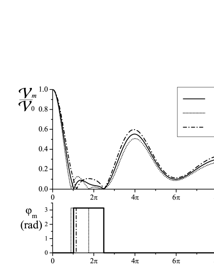
Figure 6: Calculated relative visibility and phase as a function of $J_{1}$, for a velocity distribution with a typical value of the parallel speed ratio $S_{\|}=8$ and for three values of the population unbalance parameter $\chi$: $\chi=0$ full curve; $\chi=0.1$ dash-dotted curve; $\chi=-0.1$ dotted curve. This parameter has a large effect especially when the visibility is very low.

We now calculate corrections of $J_{1}$ to describe the influence of the laboratory field $\mathbf{B}_{0}$, which is not perfectly homogeneous. We express the total magnetic field $\mathbf{B}_{tot}=\mathbf{B}_{coil}+\mathbf{B}_{0}$, where $\mathbf{B}_{coil}$ is the coil field proportional to the coil current $I_{coil}$. Its modulus is:

$$B_{tot} = \sqrt{\left(\mathbf{B}_{coil}+\mathbf{B}_{0}\right)^{2}}$$ (43)

$$\approx B_{coil}\left(1\pm\frac{\mathbf{u}\cdot\mathbf{B}_{0}}{B_{coil}}\right)$$

an approximation valid when $B_{0}\ll B_{coil}$. $\mathbf{u}$ is a local vector parallel to $\mathbf{B}_{coil}$ so that $\mathbf{B}_{coil}=\pm\mathbf{u}B_{coil}$ where the $\pm$ sign is the sign of $I_{coil}$. We split the integral giving $J_{1}$ in two regions, the region where the coil field is dominant ($in$) and the region where the laboratory field is dominant ($out$):

$$J_{1} \approx \frac{\mu_{B}}{\hbar v}\left[\int_{in}\frac{\partial B_{coil}}{\partial x}\delta x(z)dz\pm\int_{in}\frac{\partial\mathbf{u}\cdot\mathbf{B}_{0}}{\partial x}\delta x(z)dz\right.$$ (44)

$$\left.+\int_{out}\frac{\partial B_{0}}{\partial x}\delta x(z)dz\right]$$

The first term, proportional to $\left|I_{coil}\right|$, is written $A_{J1,coil}\left|I_{coil}\right|$. The second term is constant and it is convenient to write it $-A_{J1,coil}I_{0,coil}$ which defines a quantity $I_{0,coil}$ homogeneous to a current. The third term is independent of the current in the coil and we write it $J_{0,coil}$. In this way, we get:

$$J_{1}=A_{J1,coil}\left|I_{coil}-I_{0,coil}\right|+J_{0,coil}$$ (45)

It is important to note that $J_{0,coil}$ depends on the coil because of integration in the $out$ region. We call $J_{0}$ the integral as in equation (44) extended to the whole interferometer:

$$J_{0} = \frac{\mu_{B}}{\hbar v}\int\frac{\partial B_{0}}{\partial x}\delta x(z)dz$$ (46)

We need a formula which interpolates smoothly when $I_{coil}$ varies. When $I_{coil}\rightarrow 0$, the quantity $J_{1}$ must tend toward $J_{0}$. This property is verified by eq. (45) if we take $J_{0,coil}=J_{0}-A_{J1,coil}\left|I_{0,coil}\right|$. Finally, as we use two coils, a main coil (current $I$) and a compensator coil (current $I_{C}$), we generalize eq. (45) which becomes:

$$J_{1}=A_{J1}\left|I-I_{0}\right|+A_{J1,C}\left|I_{C}-I_{0,C}\right|+J_{0,I+C}$$ (47)

where $J_{0,I+C}=J_{0}-A_{J1}\left|I_{0}\right|-A_{J1}\left|I_{0,C}\right|$. To establish eq. (47), we must assume that the ($in$) regions of the two coils do not overlap, which is satisfied by our experimental apparatus LepoutrePhD ; LepoutreXXX . Eq. (47) will be used to fit experimental data.

VI.4 The case of larger magnetic fields

We consider here only $J_{1}$ and $J_{2}$ to simplify the equations. The complex visibility is then given by:

$$\frac{\underline{\mathcal{V}}}{\mathcal{V}_{0}} = \frac{1}{4}\left[(1+\chi)\left(\cos\left(J_{2}\right)+2\cos\left(\frac{3J_{2}}{4}\right)\cos\left(\frac{J_{1}}{2}\right)\right)\right.$$

$$\left.+(1-3\chi)\cos\left(J_{1}\right)\right]$$

$$+i\chi\left[\sin\left(J_{2}\right)+2\cos\left(\frac{J_{1}}{2}\right)\sin\left(\frac{3J_{2}}{4}\right)\right]$$

In fig. 7, we have plotted the complex fringe visibility as a function of the magnetic field inhomogeneity. When $\chi=0$, the imaginary part of $\underline{\mathcal{V}}$ almost vanishes but it differs slightly from $0$ because we have taken into account the nuclear spin contribution (an effect neglected in eq. (VI.4)). When $\chi$ differs from $0$, the imaginary part is not at all negligible and the fringe phase may be large, of the order of $1$ rad, when the real part of the visibility is small.

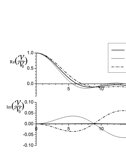
Figure 7: Calculated real and imaginary parts of the complex visibility $\underline{\mathcal{V}}/\mathcal{V}_{0}$ as a function of the coil current $I$. We use the values $J_{1}/I=0.5$ rad/A and $J_{2}/I^{2}=0.01$ rad/A², which are close to our experimental values. Same $S_{\|}$ and $\chi$ values as in fig. 6.

We should also calculate corrections to $J_{2}$ and $J_{3}$ for the inhomogeneity of the laboratory field, but these refinements are expected to be of weak influence and did not appear to improve the quality of the fits. As a consequence, only the correction to $J_{1}$ given by eq. (47) have been taken into account.

VII The Aharonov-Casher phase shift

As explained above, the Aharonov-Casher phase $\varphi_{AC}$, given by eq. (2), can be considered as being due to the motional magnetic field $\mathbf{B}_{mot}=\mathbf{E}\times\mathbf{v}/c^{2}$. This field is usually very small, $B_{mot}\approx 10^{-8}$ T for our largest electric field $E_{max}\approx 0.8$ MV/m and $v=v_{m}=1065$ m/s, but it has opposite values on the two interferometer arms as we use opposite electric fields. In practice, $B_{mot}$ is always smaller than $10^{-3}$ of the magnetic field and only the component of $B_{mot}$ parallel to this local magnetic field can play a role, but it cannot be neglected. The magnetic moment $\mu(F,m_{F})$ of the $F,m_{F}$ sublevel is a function of the magnetic field $\mathbf{B}$. We introduce a vector $\mathbf{u}_{tot}=\mathbf{B}/B$ parallel to the total magnetic field at the location $\mathbf{r}$, and we approximate the magnetic dipole moment value by using an expansion similar to eq. (39):

$$\boldsymbol{\mu}(F,m_{F}) = \mu(F,m_{F})\mathbf{u}_{tot}$$

$$\mbox{with }\mu(F,m_{F}) = \mp\mu_{B}\frac{m_{F}+2X}{2\sqrt{1+m_{F}X+X^{2}}}$$ (49)

$$\approx \mp\mu_{B}\left[\frac{m_{F}}{2}+\left(1-\frac{m_{F}^{2}}{4}\right)X\right.$$

$$+ \left.\frac{3m_{F}}{4}\left(\frac{m_{F}^{2}}{4}-1\right)X^{2}\right]$$

with the notations of eq. (VI.1). We then use equation (2) to calculate the AC phase shift as a function of $F$, $m_{F}$.

VIII Summary of the various phase shifts

In this section, we rapidly review the various phase shifts discussed in the previous sections and we estimate their magnitude in our experimental setup. We also explain their effects on the fringe visibility. The phase $\varphi_{p}$ in equation (18) is the sum of 5 contributions:

$$\varphi_{p} = \varphi_{Sagnac}+\varphi_{S}+\varphi_{Z}\left(F,m_{F}\right)$$ (50)

$$+\varphi_{AC}(F,m_{F})+\varphi_{HMW}$$

Phase Shift	Maximum value	Dependence	Effect on
	(rad)	with $F$, $m_{F}$	fringe visibility
Sagnac	$0.64$	no	negligible
Polarizability	$\approx 0.1$	no	weak
Zeeman	$\approx 10$	yes	strong
AC	$0.07$	yes	weak
HMW	$0.027$	no	no

Table 1: The phase shifts present in our experiment: for each phase shift, we give its value for the maximum fields $E_{max}\approx 0.8$ MV/m and $B_{max}\approx 14$ mT available in the interaction region used for the detection of the HMW phase, the existence of a dependence with the sublevel and its effect on the fringe visibility.

Let us discuss each term separately:

• the Sagnac phase shift $\varphi_{Sagnac}$ due to Earth rotation is easily calculated from the latitude of our experiment and the size of the interferometer:

  $$\varphi_{Sagnac}=688/v$$ (51)

  where $v$ is the atom velocity in m/s and $\varphi_{Sagnac}$ is measured in rad. With $v_{m}=1065$ m/s, this phase is rather small, $\varphi_{Sagnac}\approx 0.65$ rad JacqueyPRA08 and, as its dispersion is solely due to its velocity dependence, it has only minor effects on the fringe visibility $\mathcal{V}$.

• the Stark phase shift $\varphi_{S}$ can be very large, about $300$ rad if we applied the largest electric field $E=0.8$ MV/m on one arm only. Because of its velocity dependence, $\varphi_{S}\propto 1/v$, the fringe visibility $\mathcal{V}$ decreases when $\varphi_{S}$ increases and becomes very small for $\varphi_{S}>30$ rad because the velocity distribution of our atomic beam has a relative full width of the order of $25$%. In order to measure the HMW phase, we need the best possible fringe visibility and we tune the electric fields on the two arms so that the mean $\varphi_{S}$ is of the order of $100$ mrad. The reduction of fringe visibility due to the velocity averaging is then completely negligible but, because of defects of the geometry of the two capacitors, the $y$-dependence of $\varphi_{S}(y)$ discussed above induces a minor reduction of the fringe visibility.

• the Zeeman phase shift $\varphi_{Z}\left(F,m_{F}\right)$ would be extremely large, about $10^{5}$ rad if our maximum field $B=14$ mT was applied on one interferometer arm only, but with a relative field difference $\delta B/B\sim 10^{-4}$ between the two interferometer arms, the Zeeman phase shift is reduced to about $10$ rad for the $F=2,m_{F}=\pm 2$ sublevels. Because of the dependence of $\varphi_{Z}$ with $F,m_{F}$ and with the atom velocity, $\varphi_{Z}\propto 1/v^{2}$, this phase shift would still be sufficient to reduce the fringe visibility to a very small value. A compensating coil creating an opposite field gradient between the two interferometer arms is necessary to preserve a good visibility but, because of non-linear Zeeman effect due hyperfine uncoupling, this compensation is not complete.

• the Aharonov-Casher phase shift $\varphi_{AC}(F,m_{F})$ is a function of the $F$, $m_{F}$ sublevel and it is largest for the $F=2$, $m_{F}=\pm 2$ sublevels. Because of its geometric character, it is independent of the atom velocity. For our largest electric field, $\varphi_{AC}(F=2,m_{F}=2)\approx 70$ mrad. Because of its $F,m_{F}$-dependence, the AC phase shift has a weak but detectable effect on the fringe visibility.

• the He-McKellar-Wilkens phase shift $\varphi_{HMW}$ is independent of the $F,m_{F}$ hyperfine sublevel and of the atom velocity, because of its geometric character. For our largest electric and magnetic fields, $\varphi_{HMW}\approx 27$ mrad. As the HMW phase shift is not dispersed, it has no effect on the fringe visibility.

Table 1 summarizes the main properties of these phase shifts present in our experiment. We have two comments. The existence of phase shifts larger than the one we want to measure is not a problem as long these large phase shifts are stable: in order to observe the weak HMW phase shift, we subtract the phase shift due to the electric field and the one due to the magnetic field from the one observed when both fields are applied. The real problem comes from the fact that the signal is the sum of the signals due to 8 hyperfine sublevels and, as shown by equation (IV.4), the weights of the sublevel $j$ is the product $P_{j}\mathcal{V}_{j}$. The visibility $\mathcal{V}_{j}$ varies with the applied perturbations and this is the basis of systematic effects analyzed in section IV.

IX Conclusion

In this paper, we have recalled what are the topological phases of electromagnetic origin, namely the Aharonov-Bohm, the Aharonov-Casher and He-McKellar-Wilkens phases and the theoretical connections between these various effects. We have also discussed the possible detection schemes of the HMW phase and we have explained the principle of our experiment based on a separated-arm lithium-atom interferometer.

During our experiment, which is briefly described in ref. LepoutrePRL12 (with more details in the companion paper HMWII LepoutreXXX ), we have observed unexpected stray phases: most of them have been explained by our calculations and they result from phase-averaging effects due to experimental defects. We have discussed these effects on general grounds in section IV.

In order to develop a model of our experiment, we have analyzed in detail the Stark and Zeeman effective Hamiltonian in the ²S_1/2 ground state of ⁷Li atom and we have discussed the validity of several approximations. We have thus shown that we may assume that the Stark shift is independent of the $F,m_{F}$ sublevel and that the diamagnetic term is negligible. We have explained why we use a first-order calculation of the Stark and Zeeman phases. We have also discussed in detail the phase shifts resulting of the inhomogeneities of the electric or magnetic fields and the consequences of these phase shifts on the fringe phase and visibility. Finally, we have evaluated the Aharonov-Casher phase in our experiment and shown that it is small but not fully negligible.

X Appendix A: Relative contributions of the $F,m_{F}$ sublevels to the signal

In this appendix, we discuss various effects which may modify the relative populations of the $F,m_{F}$ sublevels.

X.1 The populations of the $F,m_{F}$ sublevels in the incident atomic beam

The atomic beam, when it enters the atom interferometer, is not optically pumped. We may assume that the $8$ Zeeman-hyperfine sublevels are equally populated for the following reasons: the only effects which could induce a partial selection of the internal states are the supersonic expansion and Stern-Gerlach forces and they are too weak to play a role in our experiment.

Supersonic expansions are well known to align the rotational angular momentum of molecules by collisions with the carrier gas, because the collisions between the seeded molecule and the carrier gas are not isotropically distributed, an anisotropy due to the velocity difference between the two species (the so-called velocity slip effect). A similar effect can align an atomic angular momentum. However, lithium atom in its ground state is in a spin $1/2$ state which cannot be aligned. Nuclear spins are uncoupled during a collision, because of the weakness of the hyperfine Hamiltonian with respect to a typical collision duration, below $10^{-12}$ s, so that collisions are not expected to align the total angular momentum $\mathbf{F}$.

Stern-Gerlach forces due to a magnetic field gradient can deflect differently the various $F,m_{F}$ sublevels and a $F,m_{F}$-dependent deflection can produce a population unbalance between these sublevels. The only places where such a deflection could occur are in the collimation slits and this would require a magnetic field gradient of the order of $10^{3}$ Tesla/m. We have chosen to use collimation slits made of silicon, a non-ferromagnetic material, so that the magnetic field gradient is surely very small.

X.2 The transmission of the interferometer

As we are using linear polarization of the laser standing waves and as the hyperfine structure of the ²P first resonance state of lithium is quite small, the diffraction amplitude is independent of $m_{F}$ for a given $F$ level ChampenoisPhD . This is true even in the presence of a weak magnetic field, comparable to the Earth field, $4\times 10^{-5}$ T, because the Zeeman splitting of the transitions, of the order of $1$ MHz in frequency units, is negligible with respect to the laser frequency detuning $\delta_{L}/(2\pi)\sim 2$ GHz MiffreEPJD05 .

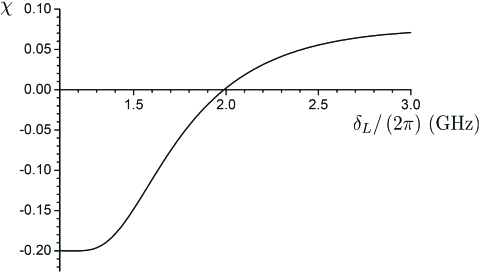
Figure 8: The population unbalance parameter $\chi$ as a function of laser frequency detuning $\delta_{L}/(2\pi)$ GHz as given by the simple model (eq. 54). The $\beta$ parameter has been taken equal to $\beta/(2\pi)=3.65$ GHz, which is optimum for a detuning $\delta_{L}/(2\pi)=2$ GHz.

The diffraction amplitude still depends on $F$ because the laser frequency detuning is not the same for the two hyperfine levels, the ground state hyperfine splitting being equal to $\omega_{HFS}/(2\pi)=0.803$ GHz in frequency units. We define the population unbalance by writing the relative population $P(F,m_{F})$ of the $F,m_{F}$ sub-level in the form:

$$P(F,m_{F}) = \left(1+5\chi\right)/8\mbox{ if }F=1$$

$$P(F,m_{F}) = \left(1-3\chi\right)/8\mbox{ if }F=2$$ (52)

The total population is normalized and the unbalance parameter $\chi$ must verify $-1/5\leq\chi\leq 1/3$ so that $P(F,m_{F})\geq 0$. We have developed a simplified model of the interferometer transmission, neglecting the variation of the diffraction amplitudes with the atom velocity vector (the modulus of the velocity has a distribution given by eq. 19, with $S_{\|}\approx 8$ and the direction of the velocity vector is characterized by an angular distribution with a full width at half maximum close to $20$ $\mu$rad). In this way, we can write the first-order diffraction amplitude by the $i^{th}$ laser standing wave in the form:

$$\left|\alpha_{i}\right| = \sin\left(\beta_{i}/\delta_{L}(F)\right)$$

$$\mbox{with }\delta_{L}(F=1) = \delta_{L}$$

$$\mbox{and }\delta_{L}(F=2) = \delta_{L}+\omega_{HFS}$$ (53)

where $\beta_{i}$ is a parameter proportional to the integral of the laser power density seen by an atom which crosses the $i^{th}$ laser standing wave. We assume that the $\beta_{i}$ parameters are optimum for a Mach Zehnder interferometer with $\beta_{2}=2\beta_{1}=2\beta_{3}=\beta$. The transmission of the interferometer is proportional to $\left|\alpha_{i}\right|^{4}$ and we thus get the unbalance parameter $\chi$:

$$\chi=\frac{\sin^{4}\left(\beta/\delta_{L}\right)-\sin^{4}\left(\beta/\left(\delta_{L}+\omega_{HFS}\right)\right)}{3\sin^{4}\left(\beta/\delta_{L}\right)+5\sin^{4}\left(\beta/\left(\delta_{L}+\omega_{HFS}\right)\right)}$$ (54)

The variations of the unbalance parameter $\chi$ are plotted as a function of the laser detuning $\delta_{L}$ in fig. 8, for a typical value of the experimental parameter $\beta$.

XI Appendix B: the Stark phase including capacitor defects

The Stark phase $\varphi_{i}(y)$, given by eq. (34), is proportional to the integral $\int E_{i}^{2}(y,z)dz$. We use an overline $\bar{...}$ to note the average over $z$ defined by the integral over the capacitor length $L_{i}(y)$, for instance, $\bar{h}_{i}(y)=\int h_{i}(y,z)dz/L_{i}(y)$ and we note $\delta_{i}(y,z)$ the dimensionless deviation from a plane capacitor defined by $h_{i}(y,z)=\bar{h}_{i}(y)\left[1+\delta_{i}(y,z)\right]$. By definition, $\bar{\delta}_{i}(y)=0$ and we assume that $\delta_{i}(y,z)\ll 1$. We also define $\bar{V}_{c,i}(y)=\int V_{c,i}(y,z)dz/L_{i}(y)$.

To calculate the Stark phase $\varphi_{i}(y)$, we expand the electric field $E_{i}(y,z)$ up to first order in $\delta_{i}(y,z)$ and in $V_{c,i}(y,z)/V_{i}$. Both assumptions are excellent, first because the design of the capacitors ensures $\delta_{i}\ll 1$, secondly because the contact potential term is of the order of $\pm 100$ mV while the applied voltage $V_{i}$ is of the order of $100$ V at least (when $V_{i}=0$, the Stark phase solely due to contact potentials, of the order of $10^{-5}$ rad at most, is completely negligible). Then $E_{i}^{2}(y,z)$ is given by:

$$E_{i}^{2}(y,z) \approx \frac{V_{i}^{2}}{\left(\bar{h}_{i}(y)\right)^{2}}\left[1+2\frac{V_{c,i}(y,z)}{V_{i}}-2\delta_{i}(y,z)\right]$$ (55)

The phase $\varphi_{i}(y)$ is obtained by integration over $z$:

$$\varphi_{i}(y) \approx \frac{2\pi\epsilon_{0}\alpha V_{i}^{2}}{\hbar v}\frac{L_{i}(y)}{\left(\bar{h}_{i}(y)\right)^{2}}\left[1+2\frac{\bar{V}_{c,i}(y)}{V_{i}}\right]$$ (56)

We introduce $\eta_{i}(y)$ which measures the $y$-dependence of the $z$-integrated geometrical defect of the capacitor $i$. $\eta_{i}(y)$ measures the relative $y$-variation of the $z$-averaged thickness of the capacitor $i$; it is defined by:

$$\frac{L_{i}(y)}{\left(\bar{h}_{i}(y)\right)^{2}}=\left<\frac{L_{i}}{\bar{h}_{i}^{2}}\right>\left[1+\eta_{i}(y)\right]$$ (57)

where $\left<...\right>$ denotes the $y$-average with the weight function $P(y)$. By definition, $\left<\eta_{i}\right>=0$. We get:

$$\varphi_{i}(y) \approx \varphi_{0i}\left[1+\eta_{i}(y)+2\frac{\bar{V}_{c,i}(y)}{V_{i}}\right]$$

$$\mbox{with }\varphi_{0i} = \frac{2\pi\epsilon_{0}\alpha V_{i}^{2}}{\hbar v}\left<\frac{L_{i}}{\bar{h}_{i}^{2}}\right>$$ (58)

In the HMW detection experiments discussed in HMWII LepoutreXXX , the voltage ratio $V_{l}/V_{u}$ is tuned so that it compensates the fact that the two capacitors have not exactly the same value of the quantity $\left<L_{i}/\bar{h}_{i}^{2}\right>$. In this way we get $\left|\left<\varphi_{l}\right>/\left<\varphi_{u}\right>-1\right|<10^{-3}$. Hence for the defect terms which are expressed by a first order expansion, it is justified to use the mean value $\varphi_{0}$ of the induced phases $\varphi_{0i}$ and the mean value $V$ of the voltages $V_{i}$. We thus obtain the Stark phase shift, including the influence of the capacitor defects:

$$\varphi_{S}(y) = \varphi_{0l}-\varphi_{0u}+\left<\varphi_{Sc}\right>$$ (59)

$$+\delta\varphi_{Sg}(y)+\delta\varphi_{Sc}(y)$$

In eq. (59), the mean phase shift (first line) is given by:

$$\left<\varphi_{S}\right> = \varphi_{0l}-\varphi_{0u}+\left<\varphi_{Sc}\right>$$

$$\mbox{with }\left<\varphi_{Sc}\right> = 2\varphi_{0}\left[\frac{\left<\bar{V}_{c,l}\right>-\left<\bar{V}_{c,u}\right>}{V}\right]$$ (60)

The term $\left(\varphi_{0l}-\varphi_{0u}\right)$, which is dominant if the voltage ratio $V_{u}/V_{l}$ is not perfectly tuned, scales like $V^{2}$. The mean term due to the contact potentials $\left<\varphi_{Sc}\right>$, which is expected to be considerably smaller, scales like $V$. The dispersion of the Stark phase shift with the atom trajectory is described by the terms of the type $\delta\varphi(y)$ (second line of eq. 59), with $\left<\delta\varphi\right>=0$. The dispersion due to geometrical defects scale like $V^{2}$, while that due to the contact potentials scale with $V$:

$$\delta\varphi_{Sg}(y) = \varphi_{0}\left[\eta_{l}(y)-\eta_{u}(y)\right]$$

$$\delta\varphi_{Sc}(y) = 2\varphi_{0}\frac{\bar{V}_{c,l}(y)-\bar{V}_{c,u}(y)}{V}-\left<\varphi_{Sc}\right>$$ (61)

Although we expect the dispersion originating from the contact potentials to be smaller, and to exhibit weak correlations because of rapid small-scale variations, its influence could not be ruled out prior to our experiment.

References

- (1) X.-G. He and B.H.J. McKellar, Phys. Rev. A 47, 3424 (1993).
- (2) K.A. Milton, Rep. Prog. Phys. 69, 1637 1711 (2006).
- (3) M. Wilkens, Phys. Rev. Lett. 72, 5 (1994).
- (4) Y. Aharonov and A. Bohm, Phys. Rev. 115, 485 (1959).
- (5) Y. Aharonov and A. Casher, Phys. Rev. Lett. 53, 319 (1984).
- (6) S. Lepoutre, A. Gauguet, G. Tr nec, M. Büchner and J. Vigué, Phys. Rev. Lett. 109, 120404 (2012).
- (7) S. Lepoutre, J. Gillot, A. Gauguet, M. Büchner and J. Vigué, companion paper HMWII submitted at the same time as the present paper.
- (8) M.V. Berry, Proc. R. Soc. Lond. A392, 45–57 (1984).
- (9) A. Shapere and F. Wilczek, Geometric Phases in Physics (World Scientific ed., Singapore, 1989).
- (10) H. Erlichson, Am. J. Phys. 38, 162 (1970).
- (11) S. Olariu and I. Iovitzu Popescu, Rev. Mod. Phys. 57, 339–436 (1985).
- (12) R.G. Chambers, Phys. Rev. Lett. 5, 3 (1960).
- (13) A. Tonomura et al., Phys. Rev. Lett. 56, 792 (1986).
- (14) M. Peshkin and A. Tonomura The Aharonov-Bohm Effect (Springer-Verlag, New York, 1989).
- (15) J. Anandan, Phys. Rev. Lett. 48, 1660 (1982).
- (16) A.G. Klein, Physica 137B, 230 (1986).
- (17) T.H. Boyer, Phys. Rev. A 36, 5083 (1987).
- (18) Y. Aharonov et al., Phys. Rev. A 37, 4052 (1988).
- (19) B. Reznik and Y. Aharonov, Phys. Rev. D 40, 4178 (1989).
- (20) A.S. Goldhaber, Phys. Rev. Lett. 62, 482 (1989).
- (21) J. Anandan, Phys. Lett. A 138, 347 (1989).
- (22) L. Vaidman, Am. J. Phys. 58, 978 (1990).
- (23) J.Q. Liang and X.X. Ding, Phys. Rev. Lett. 63, 831 (1989).
- (24) 4] J.Q. Liang, et al., Mod. Phys. Lett. A 5, 2361 (1990).
- (25) C.R. Hagen, Phys. Rev. Lett. 64, 2347 (1990).
- (26) C.R. Hagen, Intern. J. Mod. Phys. A 6, 3119 (1991).
- (27) H. Rubio, J.M. Getino and O. Rojo, Nuovo Cimento B 106, 407 (1991).
- (28) R. Mignani, J. Phys. A: Math. Gen. 24, L421 (1991).
- (29) A.S. Goldhaber and S.A. Kivelson, Phys. Lett. B 255, 445 (1991).
- (30) A. Zeilinger, R. Gähler and M.A. Horne, Phys. Lett. A 154, 93 (1991).
- (31) X.-G. He and B.H.J. McKellar, Phys. Lett. B 256, 250 (1991).
- (32) X.-G. He and B.H.J. McKellar, Phys. Lett. B 264, 129 (1991).
- (33) B. Holstein, Am. J. Phys. 59, 1080 (1991).
- (34) J.Q. Liang, Int. J. Mod. Phys. 7, 4747 (1992).
- (35) Y.D. Han and I.G. Koh, Phys. Lett. A 167 341 (1992).
- (36) G. Spavieri and G. Cavalleri, Europhys. Lett. 18, 301 (1992).
- (37) J.Q. Liang and X.X. Ding, Phys. Lett. A 176 165 (1993).
- (38) N.F. Ramsey, Phys. Rev. A 48, 80 (1993).
- (39) A.V. Balatsky and B.L. Altshuler, Phys. Rev. Lett. 70, 1678 (1993).
- (40) M.Y. Choi, Phys. Rev. Lett. 71, 2987 (1993).
- (41) B. Reznik and Y. Aharonov, Phys. Lett. B 315, 386 (1993).
- (42) G. Spavieri, Nuovo Cimento B 109, 45 (1994).
- (43) T.-Y. Lee and C.M. Ryu, Phys. Lett. A 194, 310 (1994).
- (44) M. Peshkin and H.J. Lipkin, Phys. Rev. Lett. 74, 2847 (1995).
- (45) S.M. Al-Jaber, Nuovo Cimento B 110, 1003 (1995).
- (46) T.-Y. Lee, Mod. Phys. Lett. B 10, 795 (1996).
- (47) G.R. Freeman and N.H. March, Eur. J. Phys. 18, 290 (1997).
- (48) M. Peshkin, Found. of Phys. 29, 481 (1999).
- (49) Y. Aharonov and B. Reznik, Phys. Rev. Lett. 84, 4790 (2000).
- (50) G. Spavieri, Nuovo Cimento B 115, 245 (2000).
- (51) J.A. Swansson and B.H.J. McKellar, J. Phys. A: Math. Gen. 34, 1051 (2001).
- (52) T.H. Boyer, Found. of Phys. 32, 1 (2002).
- (53) P. Hyllus and E. Sjöqvist, Phys. Rev. Lett. 89, 198901 (2002).
- (54) Y. Aharonov and B. Reznik, Phys. Rev. Lett. 89, 198902 (2002).
- (55) S. Dulat and K. Ma, Phys. Rev. Lett. 108, 070405 (2012).
- (56) R.P. Feynman, Rev. Mod. Phys. 20, 367 (1948).
- (57) P. Storey and C. Cohen-Tannoudji, J. Phys. II France 4, 1999 (1994).
- (58) A. Cimmino, G.I. Opat, A.G. Klein, H. Kaiser, S.A. Werner, M. Arif and R. Clothier, Phys. Rev. Lett. 63, 380 (1989).
- (59) H. Kaiser et al., Physica 151B, 68 (1988).
- (60) R.C. Casella, Phys. Rev. Lett. 65, 2217 (1990).
- (61) K. Sangster, E.A. Hinds, S.M. Barnett and E. Riis, Phys. Rev. Lett. 71, 3641 (1993).
- (62) K. Sangster, E.A. Hinds, S.M. Barnett, E. Riis, and A.G. Sinclair , Phys. Rev. A 51, 1776 (1995).
- (63) N.F. Ramsey, Phys. Rev. 78, 695 (1950).
- (64) K. Zeiske, G. Zinner, F. Riehle and J. Helmcke, Appl. Phys. B 60, 205 (1995).
- (65) A. Görlitz, B. Schuh and A .Weis, Phys. Rev. A 51, R4305 (1995).
- (66) S. Yanagimachi et al., Phys. Rev. A 65, 042104 (2002).
- (67) W.J. Elion et al., Phys. Rev. Lett. 71, 2311 (1993).
- (68) J.P. Dowling, C.P. Williams and J.D. Franson, Phys. Rev. Lett. 83, 2486 (1999).
- (69) C.-C. Chen, Phys. Rev. A 51, 2611 (1995).
- (70) H. Wei, R. Han and X.Wei, Phys. Rev. Lett. 75, 2071 (1995).
- (71) J. Yi, G.S. Jeon and M.Y. Choi, Phys. Rev. B 52, 7838 (1995).
- (72) G. Spavieri, Nuovo Cimento B 111, 1069 (1996).
- (73) Q. Liu, X. Huang and S. Qian, Chin. Phys. Lett. 12, 327 (1995).
- (74) C.R. Hagen, Phys. Rev. Lett. 77, 1656 (1996).
- (75) H. Wei, X.Wei and R. Han, Phys. Rev. Lett. 77, 1657 (1996).
- (76) G. Spavieri, Phys. Rev. Lett. 81, 1533 (1998).
- (77) M. Wilkens, Phys. Rev. Lett. 81, 1534 (1998).
- (78) U. Leonhardt and M. Wilkens, Europhys. Lett. 42, 365 (1998).
- (79) J. Audretsch and V.D. Skarzhinsky, Phys. Lett. A 241, 7 (1998).
- (80) J. Audretsch and V.D. Skarzhinsky, Phys. Rev. A 60, 1854 (1999).
- (81) U. Leonhardt Phys. Lett. A 253, 370 (1999).
- (82) J. Audretsch and V.D. Skarzhinsky, Phys. Lett. A 253, 373 (1999).
- (83) G. Spavieri, Phys. Rev. A 59, 3194 (1999).
- (84) G. Spavieri, Phys. Rev. Lett. 82, 3932 (1999).
- (85) V.M. Tkachuk, Phys. Rev. A 62, 052112 (2000).
- (86) J. Anandan, Phys. Rev. Lett. 85, 1354 (2000).
- (87) T.-Y. Lee, Phys. Rev. A 62, 064101 (2000).
- (88) T.-Y. Lee, Phys. Rev. A 64, 032107 (2001).
- (89) G. Spavieri, Phys. Lett. A 310, 13 (2003).
- (90) C. Furtado, Phys. Rev. A 69, 064104 (2004).
- (91) T. Ivezić, Phys. Rev. Lett. 98, 108901 (2007).
- (92) Y. Sato and R. Packard, Journal of Physics : Conference Series 150, 032093 (2009).
- (93) S. Lepoutre PhD thesis, Université P. Sabatier (2011), available on http://tel.archives-ouvertes.fr/
- (94) A. Miffre, M. Jacquey, M. Büchner, G. Trénec and J. Vigué, Eur. Phys. J. D 33, 99 (2005).
- (95) A. Miffre, PhD thesis, Universit P. Sabatier (2005), available on http://tel.archives-ouvertes.fr/
- (96) M. Jacquey, A. Miffre, M. Büchner, G. Trénec and J. Vigué, Europhys. Lett. 77, 20007 (2007).
- (97) J. Schmiedmayer, C.R. Ekstrom, M.S. Chapman, T.D. Hammond, and D.E. Pritchard, J. Phys. II, France 4, 2029 (1994)
- (98) C. R. Ekstrom, J. Schmiedmayer, M. S. Chapman, T. D. Hammond, and D. E. Pritchard,, Phys. Rev. A 51, 3883 (1995)).
- (99) M. Jacquey, A. Miffre, M. Büchner, G. Trénec, J. Vigué and A. Cronin, Phys. Rev. A 78, 013638 (2008).
- (100) C. Champenois, M. Büchner, and J. Vigué, Eur. Phys. J. D 5, 363 (1999).
- (101) C. Champenois, PhD thesis, Université P. Sabatier (1999), available on http://tel.archives-ouvertes.fr/
- (102) H. Haberland, U. Buck and M. Tolle, Rev. Sci. Instrum. 56, 1712 (1985).
- (103) A. Miffre, M. Jacquey, M. Büchner, G. Trénec and J. Vigué, Eur. Phys. J. D 38, 353 (2006).
- (104) M. Puchalski, D. Kedziera, and K. Pachucki, Phys. Rev. A 84, 052518 (2011) and erratum 85, 019910(E) (2012).
- (105) P.G.H. Sandars, Proc. Phys. Soc. 92, 857 (1967).
- (106) S. Ulzega, A. Hofer, P. Moroshkin and A. Weis, Europhys. Lett. 76, 1074 (2006).
- (107) E. Simon, P. Laurent and A. Clairon, Phys. Rev. A 57, 436 (1998).
- (108) C. Ospelkaus, U. Rasbach and A. Weis, Phys. Rev. A 67, 011402(R) (2003).
- (109) J.R. Mowat, Phys. Rev. A 5, 1059 (1972).
- (110) U. Kaldor, J. Phys. B: At. Mol. Phys. 6, 71 (1973).
- (111) E. Arimondo, M. Inguscio and P. Violino, Rev. Mod. Phys. 49, 31 (1977).
- (112) Zong-Chao Yan, Phys. Rev. Lett. 86, 5683 (2001).
- (113) Zong-Chao Yan and G.W.F. Drake, Phys. Rev. A 52, 3711 (1995).
- (114) D. M. Giltner, R. W. McGowan and Siu Au Lee, Phys. Rev. A 52, 3966 (1995) and D. M. Giltner, Ph. D. thesis, University of Colorado at Fort Collins (1996), unpublished