Stability of Boolean networks: The joint effects of topology and update rules

Abstract

We study the stability of orbits in large Boolean networks with given complex topology. We impose no restrictions on the form of the update rules, which may be correlated with local topological properties of the network. While recent past work has addressed the separate effects of nontrivial network topology and certain special classes of update rules on stability, only crude results exist about how these effects interact. We present a widely applicable solution to this problem. Numerical experiments confirm our theory and show that local correlations between topology and update rules can have profound effects on the qualitative behavior of these systems.
pacs: 89.75.-k (complex systems), 05.45.-a (nonlinear dynamical systems), 64.60.aq (phase transitions in networks).

Introduction

Systems formed by interconnecting collections of Boolean elements have been successfully used to model the macroscopic behavior of a wide variety of complex systems. Examples include genetic control [1], neural networks [2], ferromagnetism [3], infectious disease spread [4], opinion dynamics [5], and applications in economics and geoscience [6]. Each of these diverse models share the same basic structure: a set of nodes, each of which has a binary state ($0$ or $1$) at a given integer time $t$, and a set of update rules that determines the state of each node at time $t+1$ given the states of the nodes at time $t$. The relationships between nodes define a graph, where an edge is drawn from node $j$ to node $i$ if the update rule for node $i$ depends on the state of node $j$.

Depending on the desired application, the model’s graph can be random [1], fully connected [2], a lattice [3], or have other complex topology [7, 8]. The states of nodes can be updated deterministically or stochastically, synchronously or asynchronously [1, 3, 2]. Finally, in cases where the update rules are considered to be randomly generated, they can be drawn from many different ensembles [9, 7, 10, 11].

One important question about a Boolean network is whether or not it is stable, i.e., whether or not small perturbations of a typical initial state tend to grow or shrink as the system evolves. This question may have important ramifications for systems biology and neuroscience: it has been hypothesized that both gene networks [12] and neural networks [13] exist near the critical border separating the stable and unstable regimes. Recently, Pomerance et al. [8] introduced the additional hypothesis that orbital stability of the gene regulatory system may be causally related to cancer. Specifically, motivated by microdissection experiments showing genetic heterogeneity in tumors [14], they suggested that mutations that promote instability may be a contributing factor for some types of cancers.

In this paper, we present and numerically verify a general method for studying the stability of large, directed Boolean networks with locally tree-like topology. Here, by a locally tree-like network we mean that, if two nodes $j$ and $i$ are connected by a short directed path from $j$ to $i$, it is very unlikely that there will exist a second such path of the same length. This allows us to make the approximation that two inputs to a node are uncorrelated. Analyses based on this approximation have been found to yield accurate results, even in cases where the network contains significant clustering [8, 15], while making an analytic treatment of the system tractable. Our results offer a means of assessing the stability of a wide variety of Boolean network systems for which, up to now, no generally effective method has been available. We demonstrate the general utility of our approach with two examples illustrating that the joint effects of network topology and update rules can have profound effects on Boolean network dynamics, which cannot be captured by previous theories.

Model

Boolean networks are discrete-state dynamical systems in which each of the $N$ nodes of a network has a binary state $x_{i}(t)=0$ or $1$ at each integer-valued time $t$, and is updated at the next time $t+1$ to a new binary state $x_{i}(t+1)$ that is determined from the time $t$ states of its network inputs. For now we assume that updates are synchronous, but in the Supporting Information (SI), we demonstrate that the stability criterion that we obtain is the same whether nodes are updated synchronously or asynchronously. Consider a node $i$ which has $K_{i}$ network inputs, $j_{1}$…$j_{K_{i}}$. The new state of node $i$ is determined by a binary-valued update rule $F_{i}$, according to $x_{i}(t+1)=F_{i}\left(x_{j_{1}}(t),\dots,x_{j_{K_{i}}}(t)\right)$. Each $F_{i}$ may be specified in the form of a “truth table” listing all the $2^{K_{i}}$ possible inputs and the corresponding output. Denoting the vector of input states to node $i$ at time $t$ as $X_{i}(t)=(x_{j_{1}}(t),\dots,x_{j_{K_{i}}}(t))$, we have

$$x_{i}(t+1)=F_{i}\left(X_{i}(t)\right).\\$$ (1)

The network structure is represented using an adjacency matrix $A$, where $A_{ij}=1$ if there is an edge $j\to i$ [that is, if $x_{i}(t+1)$ depends on $x_{j}(t)$], and $A_{ij}=0$ otherwise.

The question we address is whether the dynamics resulting from Eq. (1) are stable to small perturbations. To define stability, we assume $N\gg 1$ and consider two states, $\bm{x}(t)=(x_{1}(t),\dots,x_{N}(t))^{T}$ and ${\tilde{\bm{x}}(t)}=(\tilde{x}_{1}(t),\dots,\tilde{x}_{N}(t))^{T}$. We define the normalized Hamming distance between these two states as the fraction of the nodal values that differ for the two states,

$$H(\bm{x}(t),\tilde{\bm{x}}(t))=\frac{1}{N}\sum_{i=1}^{N}\left|x_{i}(t)-\tilde{x}_{i}(t)\right|.$$ (2)

We consider $\tilde{\bm{x}}(0)$ to be a state that is slightly perturbed from $\bm{x}(0)$, meaning that $H(\bm{x}(0),\tilde{\bm{x}}(0))\ll 1$. Stability is then defined by whether $H(\bm{x}(t),\tilde{\bm{x}}(t))$ decreases to zero or grows to ${\mathcal{O}}(1)$ as $\bm{x}(t)$ and $\tilde{\bm{x}}(t)$ evolve under Eq. (1). Our main theoretical result is a criterion for stability that accounts for the joint effects of network topology (i.e., the $A_{ij}$) and node dynamics (i.e., the functions $F_{i}$).

The stability of Boolean networks was addressed in the original work of Kauffman [1, 12], where Boolean networks were first proposed as a model for genetic dynamics. Kauffman assumed a so-called $N$-$K$ network topology in which $K_{i}$ was the same at each node, $K_{i}=K$, and the $K$ inputs to each node were chosen randomly from amongst the $(N-1)$ other nodes. Further, for each of the $2^{K}$ input states, $F_{i}$ was chosen to be $0$ or $1$ with probability $\nicefrac{{1}}{{2}}$. Derrida and Pomeau [9] later generalized this model by introducing a truth table bias $0<\bar{p}<1$ such that, for a given input, $F_{i}=1$ with probability $\bar{p}$. They also proposed a method of stability analysis for the case of “annealed” systems, described as follows. First, note that the problem that they and Kauffman were interested in was one in which the network ($A_{ij}$) and the node dynamics ($F_{i}$) are initially randomly chosen, fixed forever after, and then used to create the dynamics (“quenched randomness”). The annealed problem is different in that the random choices of the network and node dynamics are made at every time step. In contrast with the stability of the quenched system, the stability of the annealed system can be analytically determined [9]. Derrida and Pomeau conjectured that, in the large $N$ limit, the stability boundaries for the quenched and annealed situations are approximately the same. This conjecture has been very well supported by the results of numerical experiments. Later authors generalized the Derrida-Pomeau annealing approach to include a distribution of in-degrees [16, 17, 18, 19, 20], joint in-degree/out-degree distributions [21], and “canalizing” update rules [22, 7, 23].

A further significant generalization was presented in Ref. [8] in which the network is quenched (not annealed), but the update rules ($F_{i}$) are annealed using a truth table bias $\bar{p}_{i}$ that may vary from node to node. Reference [8] called this procedure “semi-annealing” and used it to study the effects of network topological properties on stability, including such factors as network degree assortativity, correlation between node degree and the node bias $\bar{p}_{i}$, and community structure. As in the case of annealing, numerical results strongly support the hypothesis that the stability of the semi-annealed (analytically treatable) system and a typical quenched system are similar [8, 10].

In what follows, we generalize the results of Ref. [10] by using a semi-annealing procedure that enables the treatment of previously inaccessible cases of substantial interest in applications. We then illustrate this new procedure using two numerical examples. The first example is primarily pedagogical. The second is more application-oriented and uses threshold rules of the form

$$x_{i}(t+1)=U{\bigg{(}}\sum_{j}w_{ij}x_{j}(t)-\theta_{i}{\bigg{)}},$$ (3)

where $U$ denotes the unit step function, $\theta_{i}$ is a threshold value, and $w_{ij}$ is a signed weight whose magnitude reflects the strength of the influence of node $j$ on node $i$ ($w_{ij}=0$ if $A_{ij}=0$) and whose sign indicates whether node $j$ “activates” or “represses” node $i$ (i.e., promotes $x_{i}$ to be 1 or 0). (This model has been considered previously in the case where the network is $N$-$K$, $\theta_{i}=0$, and $w_{ij}=\pm 1$ [24, 11, 25, 26].) Threshold networks are also commonly used to model gene regulation [27, 28], neural networks [2], and other applications.

We begin by specifying our semi-annealing procedure, which is similar to the probabilistic Boolean networks described in [29]. We assign each node $i$ an ensemble of update rules, ${\mathcal{T}}_{i}$, from which a specific update rule is randomly drawn at each time step $t$. This choice is made independently at each network node $i$, and we denote the probability of drawing update rule $f$ as $\Pr[F_{i}=f]$. The resulting dynamics may be described by the probabilities $q_{i}(X_{i})$ that the state of node $i$, given inputs $X_{i}$, will be $1$ on the next time step,

$$q_{i}(X_{i})=\sum_{f\in{\mathcal{T}}_{i}}\Pr[F_{i}=f]f(X_{i}),$$ (4)

where we have used the fact that $f\left(X_{i}\right)=0$ or $1$. It is important to note that $q_{i}(X_{i})$ is solely determined from ${\mathcal{T}}_{i}$, independent of the update rule assignments at other nodes. Thus, computation of $q_{i}(X_{i})$ is straightforward.

The advantage of this semi-annealing procedure is that the resulting dynamics are simpler to analyze than those of systems with quenched update rules. Typically, the semi-annealed dynamics described by Eq. (4) possess a single ergodic attractor, and the stability of this attractor is similar to that of typical attractors in quenched systems. We assume the existence of a single ergodic attractor in our analysis below and briefly comment on cases for which this assumption fails in the SI.

When using the semi-annealed model, the selection of deterministic update rules is replaced by the selection of an update rule ensemble for each node $i$. The choice of ${\mathcal{T}}_{i}$, like the choice of $F_{i}$ in deterministic models, depends on the particular case under study. This will be illustrated in our numerical experiments.

To measure the stability of the semi-annealed dynamics generated by Eq. (4), we begin with many initial conditions $\bm{x}(0)$ and generate orbits $\bm{x}(t)$. We imagine that the initial conditions $\bm{x}(0)$ are selected randomly according to the natural measure of the attractor; in practice, this can be achieved by time-evolving another initial condition sufficiently long that transient behavior has ceased, and then using its final state as an initial condition. For each orbit $\bm{x}(t)$, we also consider a perturbed initial condition $\bm{\tilde{x}}(0)$, obtained by randomly choosing a small fraction $\varepsilon$ of the components of $\bm{x}(0)$ and “flipping” their states. That is, if node $i$ is chosen to be flipped, then $\tilde{x}_{i}(0)=1-x_{i}(0)$. The perturbed initial condition is then used to generate a perturbed orbit $\bm{\tilde{x}}(t)$, where, for the semi-annealed case, the random update rule time sequence for each node is the same for $\bm{\tilde{x}}(t)$ and $\bm{x}(t)$. The growth or decay of the Hamming distance between $\bm{x}(t)$ and $\bm{\tilde{x}}(t)$ defines the stability of the system.

Analysis

Given an orbit on the ergodic attractor of the semi-annealed system, we define $p_{i}$ to be the fraction of time that the state $x_{i}(t)$ of node $i$ is $1$. We call $p_{i}$ the “dynamical bias” of node $i$ and regard it as the probability that $x_{i}(t)=1$ at an arbitrarily chosen time. In what follows, we first address the determination of the dynamical biases $p_{i}$, which can then be used to determine the stability of the system.

We first note that $p_{i}$ is determined by the set of probabilities $\Pr[X_{i}]$ of $i$ receiving each input vector $X_{i}$, using $p_{i}=\sum_{X_{i}}\Pr\left[x_{i}=1\left|X_{i}\right.\right]\Pr\left[X_{i}\right]$, or

$$p_{i}=\sum_{X_{i}}q_{i}(X_{i})\Pr\left[X_{i}\right],$$ (5)

where $q_{i}$ is as defined in Eq. (4). Assuming that the network topology is locally tree-like, the states of the inputs to node $i$ can be treated as statistically independent [8, 15]. Therefore, the probabilities $\Pr[X_{i}]$ are determined by the biases of $i$’s inputs. Letting ${\mathcal{J}}_{i}$ denote the set of indices of all nodes that are inputs to $i$,

$$\Pr\left[X_{i}\right]=\prod_{j\in{\mathcal{J}}_{i}}\left[x_{j}p_{j}+\left(1-x_{j}\right)\left(1-p_{j}\right)\right],$$ (6)

where we have used the fact that $x_{i}=0$ or $1$. Inserting (6) into (5) yields a set of $N$ equations for the $N$ node biases $p_{i}$. In what follows, we envision that this set of equations has been solved for the dynamical biases $p_{i}$ at each node, and we will use these biases to evaluate the stability of the network. We find that for most practical purposes, one method for solving Eqs. (5–6) for the biases $p_{i}$ is by iteration: an initial guess for each $p_{i}$ can be inserted in (6), and (5) can then be used to obtain an improved guess, and so forth, until the $p_{i}$ have converged.

We now consider the stability of the annealed system. We say that node $i$ is “damaged” at time $t$ if $x_{i}(t)$ and $\tilde{x}_{i}(t)$ differ at time $t$. We define a vector $\bm{y}(t)$ such that $y_{i}(t)$ is the probability that $i$ is damaged at time $t$, i.e.,

$$y_{i}(t)=\Pr\left[x_{i}(t)\neq\tilde{x}_{i}(t)\right].$$ (7)

Next, let $d_{i}(X_{i},\tilde{X}_{i})$ be the probability that $i$ will be damaged if its inputs in the two orbits are $X_{i}$ and $\tilde{X}_{i}$,

$$d_{i}\left(X_{i},\tilde{X}_{i}\right)=\Pr\left[x_{i}(t+1)\neq\tilde{x}_{i}(t+1)\left|X_{i}(t),\tilde{X}_{i}(t)\right.\right].$$ (8)

We have suppressed the time dependence of $X_{i}$ and $\tilde{X}_{i}$ in $d_{i}(X_{i},\tilde{X}_{i})$ since this can be expressed in terms of the time-independent update rule ensemble as

$$d_{i}\left(X_{i},\tilde{X}_{i}\right)=\sum_{f\in{\mathcal{T}}_{i}}\Pr\left[F_{i}=f\right]\cdot\left|f(X_{i})-f(\tilde{X}_{i})\right|,$$ (9)

where we have used the fact that $f(X_{i})=0$ or $1$. Note that, like $q_{i}$, $d_{i}$ depends only on ${\mathcal{T}}_{i}$, and thus is straightforward to calculate.

Marginalizing over $X_{i}$ and $\tilde{X}_{i}$ in (7) and inserting (8),

$$y_{i}(t+1)=\sum_{\phantom{\tilde{1}}X_{i}\phantom{\tilde{1}}}\sum_{\tilde{X}_{i}}\Pr\left[X_{i}(t),\tilde{X}_{i}(t)\right]d_{i}\left[X_{i},\tilde{X}_{i}\right].$$ (10)

Because we are considering the question of stability, we have assumed that $\bm{x}(t)$ and $\bm{\tilde{x}}(t)$ are close to each other in the sense of Hamming distance for small times $t$, so $y_{i}(t)\ll 1$ for all $i$. In this case we can ignore the possibility that $X_{i}(t)$ and $\tilde{X}_{i}(t)$ differ at two or more input states and drop all terms of ${\mathcal{O}}(y^{2})$. Moreover, if $\tilde{X}_{i}(t)$ and $X_{i}(t)$ are the same, $d_{i}=0$ via Eq. (9), so nothing is contributed to the sum in Eq. (10). Therefore, the only values of $\tilde{X}_{i}$ which contribute significantly to the sum are the ones in which $\tilde{X}_{i}(t)$ and $X_{i}(t)$ differ for exactly one node $j$. Let $X_{i}^{j}(t)$ be a vector which is the same as $X_{i}(t)$ except that the state of input node $j$ is flipped [$\tilde{x}_{j}(t)=1-x_{j}(t)$]. Using this notation, we can rewrite Eq. (10) as

$$y_{i}(t+1)=\sum_{j\in{\mathcal{J}}_{i}}\sum_{X_{i}}\Pr\left[X_{i}(t),X_{i}^{j}(t)\right]d_{i}\left(X_{i},X_{i}^{j}\right).$$ (11)

Furthermore, because the network is locally tree-like and the inputs to node $i$ are therefore uncorrelated,

$$\begin{split}\Pr\left[X_{i}(t),X_{i}^{j}(t)\right]&=\Pr\left[X_{i}\right]\Pr\left[x_{i}(t)\neq\tilde{x}_{j}(t)\right]\\ &=\Pr\left[X_{i}\right]y_{j}(t).\end{split}$$ (12)

When substituted into Eq. (11), this leads to

$$y_{i}(t+1)=\sum_{j\in{\mathcal{J}}_{i}}y_{j}(t)\sum_{X_{i}}\Pr\left[X_{i}\right]d_{i}\left(X_{i},X_{i}^{j}\right).$$ (13)

Since the second sum is time-independent, we can write

$$y_{i}(t+1) =\sum_{j}R_{ij}y_{j}(t)+{\mathcal{O}}(y^{2}),$$ (14a)

$$R_{ij} \equiv\sum_{X_{i}}\Pr\left[X_{i}\right]d_{i}\left(X_{i},X_{i}^{j}\right),$$ (14b)

where $R_{ij}=0$ when there is no edge from $j$ to $i$. $R_{ij}$ may be interpreted as the probability that damage will spread from node $j$ to node $i$; in analogy with the terminology of Ref. [22], we call it the effective activity of $j$ on $i$.

The average of the normalized Hamming distance over all possible perturbations and realizations of the semi-annealed dynamics is $\langle H(\bm{x}(t),\bm{\tilde{x}}(t))\rangle=\tfrac{1}{N}\sum_{i}y_{i}(t)$, so the stability of the system is determined by whether or not the elements of $\bm{y}$ grow with time. This can be determined by writing Eq. (14a) in matrix form,

$$\bm{y}(t+1)=\bm{R}\hskip 1.0pt\bm{y}(t).$$ (15)

Since the effective activities $R_{ij}$ are non-negative, and $\bm{R}$ is typically a primitive matrix, the Frobenius-Perron theorem implies that the eigenvalue of $\bm{R}$ with largest magnitude is real and positive. We denote this eigenvalue $\lambda_{R}$. If the initial perturbation has a nonzero component along the eigenvector associated with $\lambda_{R}$, as is generally the case, then for $t$ not too large, the expected Hamming distance will grow as $(\lambda_{R})^{t}$ by Eq. (15). Therefore,

$$\left.\begin{matrix}\lambda_{R}>1\text{ implies instability}\\ \lambda_{R}<1\text{ implies stability\phantom{in}}\end{matrix}\right\}.$$ (16)

One major advantage of our analysis is that, from a computational perspective, evaluating $\lambda_{R}$ is typically faster than finding the average Hamming distance through simulations. We discuss this further in the SI, along with other computational aspects of the above solution. Another potential advantage of the criterion (16) is that, in some cases, it can facilitate qualitative understanding. For example, in previous work [8], it was shown that network assortativity promotes instability for a special case of the above situation.

Numerical results

We now use the general framework presented above to analyze two cases that illustrate the effects of correlations between local topological features and update rules. In each example, we construct a single network with $N=10^{5}$ nodes using the configuration model [30]. The in-degrees are Poisson-distributed with a mean of $4$ and the out-degrees are scale-free with exponent $\gamma\approx 2.2$. In Fig. 1, we plot the average Hamming distance $\langle H\rangle$ and $\lambda_{R}$ against a tuning parameter for each model. To calculate each Hamming distance $H$, we first time-evolve a random initial condition (using a quenched set of update rules) for $100$ time steps to ensure that it is on an attractor, then apply a perturbation by flipping the values of a random fraction $\varepsilon=0.01$ of the nodes. Next we time-evolve both the original and perturbed orbits for another $400$ time steps, measuring the Hamming distance $H$ over the last $100$ of these to ensure that it has reached a steady state. We take the average $\langle H\rangle$ over $10$ initial conditions for each quenched set of update rules. In the figures, we show $\langle H\rangle$ for both a single quenched system as well as an average over $50$ sets of quenched update rules.

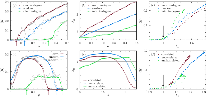
Figure 1: Normalized average Hamming distance $\langle H\rangle$ and $\lambda_{R}$ for a network with XOR, OR, and AND update rules (panels $a$–$c$) and a threshold network (panels $d$–$f$). Filled markers are averaged over $50$ quenched realizations of the thresholds, while hollow markers show a single quenched realization. Squares, circles, and triangles represent different correlations between network topology and update rules; see text for details. ($a$) When $\alpha$ is used as a tuning parameter, the stability transitions for each of the three cases are far apart. Locations where $\lambda_{R}=1$ are marked by arrows. ($b$) Viewing $\lambda_{R}$ as a function of $\alpha$, we see that this behavior agrees with the theoretical prediction for critical stability, $\lambda_{R}=1$. ($c$) Plotting $\langle H\rangle$ against $\lambda_{R}$ directly, we see that the transition for all three curves occurs at $\lambda_{R}=1$. ($d$–$f$) Results for threshold networks are shown, analogous to those in panels ($a$–$c$), using $\bar{\theta}$ as a tuning parameter rather than $\alpha$.

Example 1: XOR, OR, and AND update rules

In our first example, we illustrate the effect of correlations by assigning a node either a highly “sensitive” update rule (XOR) or a less sensitive update rule (OR or AND) based on the node’s in-degree. That is, the update rule at each node $i$ is randomly drawn from three classes: (a) XOR, whose output is one (zero) if $i$ has an odd (even) number of inputs that are one; (b) OR, whose output is one if and only if at least one input is one; or (c) AND, whose output is one if and only if all $K_{i}$ inputs are one. Following [22], we refer to XOR as highly sensitive because any single input flip will cause its output to flip, so $R_{ij}=1$ whenever there is an edge from $j$ to $i$. On the other hand, if node $i$ has OR or AND as its update rule, flipping node $j$ will cause node $i$ to flip only if every node other than $j$ is zero or one, respectively. Thus in cases (b) and (c), $R_{ij}$ depends on the node biases $p_{j}$ which are obtained by solving Eqs. (5–6). For OR, $R_{ij}=\prod_{k}(1-p_{k})$, and for AND, $R_{ij}=\prod_{k}p_{k}$, where the products are taken over all inputs $k$ which are not equal to $j$.

Figure 1($a$–$c$) shows results for a network with these three classes of update rules. We assign a fraction of nodes $\alpha$ to have XOR update rules, and the remaining nodes are evenly split between OR and AND rules. We consider three cases: (1) XOR is assigned to the $\alpha N$ nodes with the largest in-degree; (2) XOR is randomly assigned to $\alpha N$ nodes irrespective of their degrees; or (3) XOR is assigned to the $\alpha N$ nodes with smallest in-degree. In all three cases, the remainder are randomly assigned OR or AND. In numerical simulations, all update rule assignments are quenched. In order to find appropriate semi-annealing probabilities to use in our theoretical prediction, we note that the initial assignment of XOR is deterministic in cases (1) and (3), but OR and AND are assigned randomly. Therefore, in the theory, we treat the network and the identity of the XOR nodes as fixed, and anneal over the OR and AND nodes, assigning a probability of $\nicefrac{{1}}{{2}}$ to choosing either OR or AND on each time step. (Other annealing choices are also possible, but we choose this because it most straightforwardly resembles the quenched assignment of update rules above.)

As can be seen in Fig. 1($a$), the values of $\alpha$ at which the three cases become unstable are quite different, thus demonstrating that stability is strongly affected by correlation between the local topological property of nodal in-degree and the sensitive XOR update rule. As shown in Fig. 1($c$), however, when we re-plot $\langle H\rangle$ against $\lambda_{R}$, we see that in each case the network becomes unstable at $\lambda_{R}\approx 1$, as predicted by the theory. This is also strikingly illustrated by the vertical arrows in Fig. 1($a$) marking the values of $\alpha$ at which $\lambda_{R}=1$ [c.f., Fig. 1($b$)].

Example 2: Threshold networks

We now consider networks with threshold rules as given in Eq. (3); such threshold rules may be re-cast as Boolean functions $F_{i}$ by enumerating all possible $X_{i}$ and calculating whether the weighted sum of inputs exceeds the threshold $\theta_{i}$. Conversely, threshold rules are appropriate for Boolean network applications in which each edge has a fixed “activating” or “repressing” character.

Our results for threshold networks are shown in Fig. 1($d$–$f$) and are generated in the following manner. To assign the weight $w_{ij}$ for each edge $j\to i$, we first assign half of the edges to be activating and half to be repressing. Then, the weight is drawn from a normal distribution with mean $1$ (activating) or $-1$ (repressing) and standard deviation $\nicefrac{{1}}{{4}}$. We also consider two additional cases where the weights are either correlated or anticorrelated to a topological property of the network, the product of a node’s in-degree and out-degree. (Nodes with a high degree product play a crucial role in the stability of Boolean networks [31, 8, 32].) We generate the correlated and anticorrelated cases by exchanging weights between pairs of edges in the original (“uncorrelated”) case. Specifically, we repeat the following procedure. First, we select two random edges $j_{1}\to i_{1}$ and $j_{2}\to i_{2}$ in the network. Next, we identify the edge for which $i$ has a higher degree product. Finally, in the correlated (anticorrelated) case, we exchange the values of the two weights if doing so would increase (decrease) the weight going to the node with the higher degree product. We repeat this procedure $E/2$ times, where $E$ is the number of edges in the network, so that each edge is expected to be considered for one exchange.

In this example, we model the case in which the thresholds of different nodes are similar, but not necessarily equal. In the theory, we treat this case by annealing the thresholds $\theta_{i}$ over a gaussian distribution with a mean $\bar{\theta}$ and standard deviation $\sigma_{\theta}=\nicefrac{{1}}{{10}}$. By Eq. (3),

$$q_{i}(X_{i})=\Phi{\bigg{[}}\frac{1}{\sigma_{\theta}}{\bigg{(}}\sum_{j}w_{ij}x_{j}-\bar{\theta}{\bigg{)}}{\bigg{]}},$$ (17)

where $\Phi(x)=(2\pi)^{-1/2}\int_{-\infty}^{x}\exp(-t^{2}/2)\text{d}t$. Similarly, we find that $d_{i}(X_{i},X_{i}^{j})=|q_{i}(X_{i})-q_{i}(X_{i}^{j})|$. These expressions can be used to calculate $p_{i}$, $R_{ij}$, and $\lambda_{R}$ using Eqs. (5–6,14). (Here, as in many cases, it is not necessarily to list the ensemble of update rules ${\mathcal{T}}_{i}$ explicitly, because $q_{i}$ and $d_{i}$ can be calculated directly.) In our numerical simulations, we treat $\theta_{i}$ as quenched by writing $\theta_{i}=\bar{\theta}+\delta\theta_{i}$, where $\delta\theta_{i}$ is drawn from a normal distribution with mean $0$ and standard deviation $\sigma_{\theta}$.

In Fig. 1($d$–$f$), we show results for both a single quenched set of $\delta\theta_{i}$ (hollow markers) as well as an average over $50$ quenched sets of $\delta\theta_{i}$ (filled markers). In each case, single quenched realizations show similar behavior to the average, in agreement with the semi-annealing hypothesis. More striking is the qualitative difference between the anticorrelated case and the two other cases. At low thresholds, the anticorrelated network is stable, whereas both of the other cases are unstable. As the threshold is increased, the anticorrelated network becomes unstable before becoming stable again at large thresholds. This behavior is explained in Fig. 1($e$), where we see that in all three cases, $\lambda_{R}$ initially increases with increasing $\bar{\theta}$, but it is only in the anticorrelated that $\lambda_{R}<1$ initially. Finally, in Fig. 1($f$), we re-plot the same data for $H$ against $\lambda_{R}$. We see that in all three cases the stability transition clearly occurs at $\lambda_{R}=1$, confirming our analysis.

Discussion

We have presented a general framework for predicting orbit stability in large, locally tree-like Boolean networks, given arbitrary network topology and update rules. There are three main steps in this process: (1) select update rule ensembles ${\mathcal{T}}_{i}$ (rather than deterministic rules $F_{i}$), and compute $q_{i}$ and $d_{i}$; (2) calculate the dynamical biases $p_{i}$ of the each node $i$ by iterating Eqs. (5–6); and (3) calculate the activity matrix $\bm{R}$ with elements given by Eq. (14). The largest eigenvalue of this matrix, $\lambda_{R}$, then determines the stability of the system, Eq. (16). As illustrated above, the first step requires a judicious selection of which aspects of the update rules should remain quenched, but is typically straightforward thereafter.

As examples of the application of our general stability criterion, we analyzed both a pedagogical case and the case of threshold networks, where all update rules are assumed to be of the form of Eq. (3). These results show that the stability of a Boolean network is strongly affected not only by the network topology and nodal update rules, but by correlations between the two. Although previous research into the stability of Boolean networks has primarily focused on either topology or update rules alone, Figs. 1($a$,$d$) show that correlations can have profound qualitative effects on the dynamical properties of a network. Presumably, these aspects of biological networks interact strongly during evolution, and so joint effects in topology and update rules should be analyzed carefully when studying genetic or neural systems.

Acknowledgements: This work was funded by ARO grant W911NF-12-1-0101.

Supplemental Information

Abstract

In this supplement, we explore several topics related to our stability condition for Boolean networks. We show that the stability condition is unchanged for asynchronously updated networks, discuss the conditions under which our derivation is valid, analyze the computational complexity of our solution, and calculate the critical slope of the stability transition.

Asynchronous updating

Asynchronous updates may arise in discrete state systems for several reasons. For example, links may have nonuniform delays, $\delta_{ij}$, that model delays arising from, for example, the chemical kinetics of gene regulation. In this case, the dynamics would be described by a modified version of Eq. (4) in which the state of node $i$ at time $t$ depends on the states of its inputs $j$ at times $(t-\delta_{ij})$. Another alternative is a model in which nodes are individually chosen to be updated in a stochastically determined order. Here, we show that the stability condition given in the main text applies not only to the case of synchronous nodal updates, but to asynchronous models as well, including both of these examples.

In particular, we consider update times, $\tau_{1}<\tau_{2}<...<\tau_{t}<...$, where the update intervals, $(\tau_{t+1}-\tau_{t})$, are arbitrary, incommensurate and do not influence the analysis. Since the update times are incommensurate, we approximate the deterministic choice of node to update at each time, indexed by integer $t$, with a stochastic process where node $i$ (and only node $i$) is chosen to be updated by Eq. (4) with probability $\rho_{i}$. This is, of course, also appropriate to systems that are inherently stochastic. To analyze this case, we define the vector $\bm{y}(t)$ as in the main text; however, we must make some adjustments to the approximate update equation, Eq. (14). Since node $i$ is chosen independently of the values of the nodes, the joint probability at time step $t$ that node $i$ is chosen for update and that node $i$ differs between the two initial conditions after the update is given approximately by $\rho_{i}\sum R_{ij}y_{j}(t)$. If node $i$ is not chosen for update at this time step, $y_{i}$ does not change. Putting this together, we get, for small $t$ and small initial perturbations, $y_{i}(t+1)\approx\rho_{i}\sum R_{ij}y_{j}(t)+(1-\rho_{i})y_{i}(t)$, which we rewrite in matrix form as

$$\bm{y}(t+1)=\bm{\rho}(\bm{R}-\bm{I})\bm{y}(t)+\bm{y}(t),$$

where $\bm{\rho}$ is a diagonal matrix with $\rho_{i}$ in each row, $\bm{I}$ is the identity matrix, and $\bm{R}$ is the activity matrix. In order to see that Eq. (16) also applies in this case, we note that, at criticality, $\bm{y}(t+1)=\bm{y}(t)$, so that Eq. (Asynchronous updating) reduces to $\bm{\rho}(\bm{R}-\bm{I})\bm{y}(t)=\bm{0}$. This has a solution for $\bm{y}\neq\bm{0}$ only if $\lambda_{R}=1$. Note, however, that in this case, for $\lambda_{R}>1$, the growth rate of the Hamming distance will be at a rate of the order of $1/N$ smaller than the rate of the synchronously updated networks, because $N$ time steps of asynchronous update correspond to one time step of synchronous update.

Comments on Equations (5–6)

In the main text, we make three simplifying assumptions about the derivation and solution of Eqs. (5–6):

1. The correlations between the states of different inputs to a single node are negligible, because the network is locally treelike.

2. Equations (5–6) have a single stable solution, describing the attractor of the semi-annealed dynamics.

3. This solution can be found by iterating the equations.

Here we add some comments about these assumptions and the conditions under which they are valid.

First, the locally treelike approximation has been effective in describing the structural and dynamical properties of a variety of complex networks, as documented in [15]. In particular, it has been applied successfully to Boolean networks and related percolation problems in [33, 8, 10, 34]. In this context, we may argue as follows that it allows us to assume the independence of two nodes $j_{1}$ and $j_{2}$ which are both inputs to a third node $i$. We would expect correlations between $x_{j_{1}}(t)$ and $x_{j_{2}}(t)$ to arise mainly from the two nodes being mutually influenced by a previous state of a third node, $x_{k}(t-h)$, where node $k$ has paths of length $h$ to both $j_{1}$ and $j_{2}$. But if this is the case, $k$ has two independent paths of length $h+1$ to $i$. In locally treelike networks, the number of such paths is an insignificant fraction of paths of the same length. It is hypothetically possible that this assumption may nonetheless break down in cases where the dynamics exhibit a long correlation length, as might be expected when there is a phase transition in $\langle p_{i}\rangle$. Numerically, however, we find no cause for concern. For example, such a case occurs for the threshold networks studied in Example 2 of the main text, when the stability transition at large $\bar{\theta}$ coincides with a phase transition in $\langle p_{i}\rangle$. In this case, as in all of our numerical work, we observe that the stability transition still occurs at $\lambda_{R}=1$, as predicted by theory.

We next consider the second and third assumptions above. The Brouwer fixed point theorem guarantees that Eqs. (5–6) have at least one solution, but not that it is unique or stable. Non-uniqueness does not present any difficulties for the theory; in this case, each solution represents a separate attractor, and the stability of each attractor may be determined separately. (For example, it is possible to construct threshold networks which have one solution with $p_{i}=0$ for all nodes $i$ and another solution where $p_{i}>0$ for most $i$.) A second, more troublesome scenario is that there are no stable solutions. In this case, iteration of Eqs. (5–6) would not converge to a solution but instead fluctuate periodically or chaotically. An example of this behavior occurs in networks where the update rules are chosen to approximate the logistic map. In this case, as the tuning parameter is changed, the system undergoes a period-doubling cascade. In principle the method could be extended to this situation; however, it seems unlikely that systems undergoing significant dynamics in the biases would be stable with respect to small perturbations. We note, however, that this is a rather pathological case, and that typical biological applications have stable solutions.

One final possibility is that there is a family of marginally stable solutions to Eqs. (5–6). For example, this occurs in a loop with two nodes and the the copy update function (i.e., the output is the input). In this case, iteration oscillates and does not converge, since any solution where $p_{1}=p_{2}$ is valid. We have never observed this phenomenon when $0<q_{i}(X_{i})<1$ for all $i$ and $X_{i}$, but this sometimes occurs when Eqs. (5–6) are applied directly to quenched, deterministic dynamics (i.e., $q_{i}(X_{i})=0$ or $1$ for all $i$ and $X_{i}$). However, when analyzing deterministic dynamics, one may either consider a related semi-annealed problem (that reflects, say, realistic noise models or measurement uncertainty), as we do here, or one may measure $\Pr[X_{i}]$ for a particular attractor directly from numerical simulations, then find the stability condition using Eqs. (14) and (16).

Computational Complexity

We note that the procedure presented in the main text is applicable even to very large networks. The Frobenius-Perron eigenvalue $\lambda_{R}$ may typically be found through power iteration, which requires only $\mathcal{O}(E)$ operations, where $E$ is the number of edges; for sparse networks, this is $\mathcal{O}(N)$. Another advantage of our method is that the use of dynamical biases and the locally treelike approximation offers a tremendous computational improvement over previous theoretical treatments of similar systems. For example, the analysis of probabilistic Boolean networks in Ref. [29] relies upon a state transition matrix of size $2^{N}\times 2^{N}$, which is intractable for networks with more than a few dozen nodes. In contrast, iterating Eqs. (5–6) requires fewer than ${\mathcal{O}}(N2^{K})$ steps, where $K$ is the maximum in-degree of all nodes. This is numerically feasible for large-$N$ networks as long as $K\leq 20$. In many cases, additional simplifying assumptions may offer even greater computational speed.

Critical Slope

The second-order terms in the expansion in Eq. (10) may be used to derive the critical slope of $H$ near $\lambda_{R}=1$. We include a sketch of this derivation because it may be useful for near-critical approximations or for designing networks with extreme behavior near the critical point.

To find the second-order terms in Eq. (10), we need to consider input combinations which differ for two distinct inputs $j$ and $k$, which we denote $\tilde{X}=X_{i}^{j,k}$ in analogy with our definition of $X_{i}^{j}$ in the main text. The probabilities of these input combinations are given, up to ${\mathcal{O}}(y^{2})$, by

$$\begin{split}\Pr\left[X_{i}(t),X_{i}^{j}(t)\right]&=\Pr[X_{i}]\ y_{j}(t)\left(1-\sum_{k\neq j}y_{k}(t)\right)\\ \Pr\left[X_{i}(t),X_{i}^{j,k}(t)\right]&=\Pr[X_{i}]\ y_{j}(t)\ y_{k}(t).\end{split}$$ (S2)

Following similar steps as those that led to Eq. (15), we obtain

$$\begin{split}y_{i}(t+1)&=\sum_{j}R_{ij}y_{j}(t)+\sum_{j,k}R_{ijk}y_{j}(t)y_{k}(t),\\ R_{ijk}&\equiv\frac{1}{2}\sum_{X_{i}}\Pr[X_{i}]d_{i}\left[X_{i},X_{i}^{j,k}\right]-R_{ij},\end{split}$$ (S3)

where $R_{ij}$ is defined as in the main text. Note that when $j=k$, $R_{ijk}=0$.

Now we may derive the critical slope. We consider each $y_{i}$ to have reached a steady state and hence drop the time-dependence in $y_{i}(t)$. Next we write a perturbation expansion for each variable near the critical point, $y_{i}=\varepsilon Hy_{i}^{1}+\varepsilon^{2}y_{i}^{2}$ and $\lambda_{R}=1+\varepsilon\lambda_{R}^{1}$, where superscripts for $y_{i}$ and $\lambda_{R}$ refer to the level of the perturbation expansion. From Eq. (15), $\bm{y}^{1}$ must be the right Frobenius-Perron eigenvector of the first-order $R$-matrix. Here it has been normalized so that $\sum_{i}y_{i}^{1}=1$. Inserting the second-order expansion and simplifying, we obtain

$$y_{i}^{2}=H\lambda_{R}^{1}y_{i}^{1}+\sum_{j}R_{ij}y_{j}^{2}+H^{2}\sum_{j,k}R_{ijk}y_{j}^{1}y_{k}^{1}$$ (S4)

This expression may be further simplified by using left Frobenius-Perron eigenvector of $R$, which we denote $\bm{u}$. Multiplying through by $u_{i}$ and summing over $i$, the left-hand side and the second term on the right-hand side of Eq. (S4) cancel to leading order in $\varepsilon$. With the remaining terms, we find that the critical slope $m_{c}=H/\lambda_{R}^{1}$ is

$$m_{c}=-\frac{\sum_{i}u_{i}y^{1}_{i}}{\sum_{i,j,k}R_{ijk}u_{i}y_{j}^{1}y_{k}^{1}}.$$ (S5)

This result may be used numerically to find the critical slope in particular cases, because the eigenvector $\bm{y}^{1}$ may be found along with $\lambda_{R}$. It may also be used to approximate the critical slope analytically, when good approximations for $\bm{y}^{1}$ are known, as in Refs. [8, 32].

References

- [1] S. A. Kauffman. Metabolic stability and epigenesis in randomly constructed genetic nets. J. Theor. Biol., 22(3):437–467, 1969.
- [2] J. J. Hopfield. Neural networks and physical systems with emergent collective computational abilities. Proc. Natl. Acad. Sci., 79(8):2554–2558, 1982.
- [3] Roy J. Glauber. Time-dependent statistics of the ising model. J. Math. Phys., 4(2):294–307, 1963.
- [4] M. E. J. Newman. Spread of epidemic disease on networks. Phys. Rev. E, 66(1):016128, 2002.
- [5] Claudio Castellano, Santo Fortunato, and Vittorio Loreto. Statistical physics of social dynamics. Rev. Mod. Phys., 81(2):591–646, 2009.
- [6] Barbara Coluzzi, Michael Ghil, Stéphane Hallegatte, and Gérard Weisbuch. Boolean delay equations on networks in economics and the geosciences. Int. J. Bifurcat. Chaos, 21(12):3511–3548, 2011.
- [7] Stuart Kauffman, Carsten Peterson, Björn Samuelsson, and Carl Troein. Random boolean network models and the yeast transcriptional network. Proc. Natl. Acad. Sci., 100(25):14796–14799, 2003.
- [8] Andrew Pomerance, Edward Ott, Michelle Girvan, and Wolfgang Losert. The effect of network topology on the stability of discrete state models of genetic control. Proc. Natl. Acad. Sci., 106(20):8209–8214, 2009.
- [9] B Derrida and Y Pomeau. Random networks of automata: A simple annealed approximation. Europhys. Lett., 1(2):45–49, 1986.
- [10] Andrew Pomerance, Michelle Girvan, and Ed Ott. Stability of boolean networks with generalized canalizing rules. Phys. Rev. E, 85(4):046106, 2012.
- [11] Thimo Rohlf and Stefan Bornholdt. Criticality in random threshold networks: annealed approximation and beyond. Physica A, 310(1–2):245–259, 2002.
- [12] Stuart Kauffman. The Origins of Order: Self-Organization and Selection in Evolution. Oxford Univ. Press, 1993.
- [13] Woodrow L. Shew, Hongdian Yang, Thomas Petermann, Rajarshi Roy, and Dietmar Plenz. Neuronal avalanches imply maximum dynamic range in cortical networks at criticality. J. Neurosci., 29(49):15595–15600, 2009.
- [14] Isabel González-García, Ricard V. Solé, and José Costa. Metapopulation dynamics and spatial heterogeneity in cancer. Proc. Natl. Acad. Sci., 99(20):13085–13089, 2002.
- [15] Sergey Melnik, Adam Hackett, Mason Porter, Peter Mucha, and James Gleeson. The unreasonable effectiveness of tree-based theory for networks with clustering. Phys. Rev. E, 83(3):036112, 2011.
- [16] Ricard V. Solé and Bartolo Luque. Phase transitions and antichaos in generalized kauffman networks. Phys. Lett. A, 196(1–2):331–334, 1994.
- [17] Bartolo Luque and Ricard V. Solé. Phase transitions in random networks: Simple analytic determination of critical points. Phys. Rev. E, 55:257–260, 1997.
- [18] Jeffrey J. Fox and Colin C. Hill. From topology to dynamics in biochemical networks. Chaos, 11(4):809–815, 2001.
- [19] Maximino Aldana and Philippe Cluzel. A natural class of robust networks. Proc. Natl. Acad. Sci., 100(15):8710 –8714, 2003.
- [20] Maximino Aldana. Boolean dynamics of networks with scale-free topology. Physica D, 185(1):45–66, 2003.
- [21] Deok-Sun Lee and Heiko Rieger. Broad edge of chaos in strongly heterogeneous boolean networks. J. Phys. A, 41(41):415001, 2008.
- [22] Ilya Shmulevich and Stuart A. Kauffman. Activities and sensitivities in boolean network models. Phys. Rev. Lett., 93(4):048701, 2004.
- [23] Stuart Kauffman, Carsten Peterson, Björn Samuelsson, and Carl Troein. Genetic networks with canalyzing boolean rules are always stable. Proc. Natl. Acad. Sci., 101(49):17102 –17107, 2004.
- [24] K. E. Kurten. Correspondence between neural threshold networks and kauffman boolean cellular automata. J. Phys. A, 21(11):L615, 1988.
- [25] F. Greil and B. Drossel. Kauffman networks with threshold functions. Eur. Phys. J. B, 57(1):109–113, 2007.
- [26] Agnes Szejka, Tamara Mihaljev, and Barbara Drossel. The phase diagram of random threshold networks. New J. Phys., 10(6):063009, 2008.
- [27] Fangting Li, Tao Long, Ying Lu, Qi Ouyang, and Chao Tang. The yeast cell-cycle network is robustly designed. Proc. Natl. Acad. Sci., 101(14):4781–4786, 2004.
- [28] Matthias Rybarsch and Stefan Bornholdt. Binary threshold networks as a natural null model for biological networks. Phys. Rev. E, 86(2):026114, 2012.
- [29] Ilya Shmulevich, Edward R. Dougherty, Seungchan Kim, and Wei Zhang. Probabilistic boolean networks: a rule-based uncertainty model for gene regulatory networks. Bioinformatics, 18(2):261–274, 2002.
- [30] M. E. J. Newman. The structure and function of complex networks. SIAM Review, 45(2):167–256, 2003.
- [31] D.-S. Lee and Heiko Rieger. Comparative study of the transcriptional regulatory networks of e. coli and yeast: Structural characteristics leading to marginal dynamic stability. J. Theor. Biol., 248(4):618–626, 2007.
- [32] Edward Ott and Andrew Pomerance. Approximating the largest eigenvalue of the modified adjacency matrix of networks with heterogeneous node biases. Phys. Rev. E, 79(5):056111, 2009.
- [33] Juan G. Restrepo, E. Ott, and B. R. Hunt. Weighted percolation on directed networks. Phys. Rev. Lett., 100(5):058701, 2008.
- [34] Shane Squires, Edward Ott, and Michelle Girvan. Dynamical instability in boolean networks as a percolation problem. Phys. Rev. Lett., 109(8):085701, 2012.