Experimental validation of XRF inversion code for Chandrayaan-1

Abstract

We have developed an algorithm (x2abundance) to derive the lunar surface chemistry from X-ray fluorescence (XRF) data for the Chandrayaan-1 X-ray Spectrometer (C1XS) experiment. The algorithm converts the observed XRF line fluxes to elemental abundances with uncertainties. We validated the algorithm in the laboratory using high Z elements (20 $<$ Z $<$ 30) published in Athiray et al., (2013). In this paper, we complete the exercise of validation using samples containing low Z elements, which are also analogous to the lunar surface composition (ie., contains major elements between 11 $<$ Z $<$ 30). The paper summarizes results from XRF experiments performed on Lunar simulant (JSC-1A) and anorthosite using a synchrotron beam excitation. We also discuss results from the validation of x2abundance using Monte Carlo simulation (GEANT4 XRF simulation).

1 Introduction

Solar X-rays impinge on the lunar surface and trigger XRF emission from elements in the upper layers (the major elements being viz., Mg, Al, Si, Ca, Ti and Fe). Chandrayaan-1 X-ray spectrometer (C1XS) (Grande et al.,, 2009) measured this XRF emission during several flares in the period Nov’2008 - Aug’2009. In order to convert the observed X-ray line flux determined from C1XS spectral data, a code ‘x2abundance’ is developed, where a new approach is adopted using Fundamental Parameter method (Criss & Birks,, 1968; Rousseau & Boivin,, 1998). A detailed description of the algorithm of x2abundance along with the fundamental assumptions and limitations are given in (Athiray et al.,, 2013) (here onwards Paper I). In paper I, we validated x2abundance with laboratory XRF experiments using samples containing major elements of high atomic number (20 $<$ Z $<$ 30 - set A samples). However, the major rock forming elements are low Z elements (Z $<$ 26) which makes it necessary to demonstrate the validity using samples with composition similar to the lunar surface. In this paper, we present the validation of x2abundance using XRF experiments on lunar analogues with elements in the range 11 $<$ Z $<$ 26. We also compare x2abundance results with X-ray fluorescence simulation using GEANT4, a Monte Carlo simulation tool kit.

A brief description of the laboratory XRF experiments on lunar analogue samples excited with a synchrotron beam is given in Sec. (2). Details of X-ray spectral analysis along with laboratory experimental results and validation are given in Secs.(3 and 4). GEANT4 XRF simulations, results and validation are summarized in Sec. (5). Finally, a short discussion on the complete work is presented in Sec. (6).

2 XRF experiments

The objective of the current experiment is to validate x2abundance developed for C1XS analysis using samples that are analogous to lunar surface composition. These samples contain elements from Mg to Fe whose K-shell X-ray emission energies ranges from ${\approx}$ 1.2 keV to ${\approx}$ 7.0 keV.

2.1 Sample details

Lunar surface can broadly be classified into two regions viz., (a) dark mare regions (high mafic content) and (b) bright highland regions (concentration of low dense minerals with low mafic content). The mare regions are believed to be the partial melts of lunar interior erupted on the surface. Whereas, highlands are believed to be formed during the end stages of lunar magma ocean where the lighter mineral plagioclase feldspar floated and crystallized on the surface. For our experiment, two samples which closely represent the composition of lunar mare and highland region are used. A brief description of the samples used are given here:

• Lunar Simulant (JSC-1A) : JSC-1A is a lunar mare regolith simulant released by NASA for research studies mined from a commercial cinder quarry at Merriam Crater (35^∘ 20’ N, 111^∘ 17’ W). The volcanic ash deposit of Merriam crater is basaltic in composition, similar to the soil from Maria terrain of the Moon. The mined ash was processed to produce the simulants with mean grain size of ${\approx}$ 190 ${\mu}$m. A complete characterization of lunar simulant (JSC-1A) is reported by (Ray et al.,, 2010).
  

• Sittampundi rock : This sample is taken from the anorthositic rocks available at Sittampundi (near Salem, Tamil Nadu), India, which are considered close to lunar highland rocks in composition. The plagioclase in these rock samples exhibit an anorthite content in the range An_80-100 (Anbazhagan et al.,, 2012) in comparison to that in Apollo returned samples which has an anorthite content of ${\approx}$ An₉₅ on average. Pure calcic-anorthite and labradorite are the dominant minerals in this sample. The sample exhibit a low mafic content and large concentration of Al and Ca. They are pulverized to a grain size of about 100 ${\mu}$m or smaller. Detailed studies on the rocks of this site are reported by (Anbazhagan et al.,, 2012; Aarthy et al.,, 2009).

Pellets of these samples were made after crushing them manually and compressing it with a pelletizer. We assume that the pellets are a close representation of flat and homogeneous sample. However, in reality the size distribution of soil particles on the Moon is not well characterized. It is shown already that, in heterogeneous samples, the observed XRF line strength exhibit a dependence on grain size (Maruyama et al.,, 2008; N$\ddot{a}$r$\ddot{a}$nen et al.,, 2008), which is assumed to be minimal for C1XS observations due to large spatial scales (Weider et al.,, 2012). A detailed description of experimental setup is given in the following section.

2.2 Experiment details

As the samples contain diverse elements ranging from Mg to Fe, we irradiated the samples using a high intense mono-energetic synchrotron X-ray beam. For this purpose, we have utilized the XRF-${\mu}$ probe beam-line (BL-16) at Indus-2 synchrotron beam facility, RRCAT, Indore, India. The Indus-2 electron storage ring is currently operating at 2.5 GeV with nominal current of 100 mA. BL-16 of Indus-2 is installed on the 5^∘ port of bending magnet and operates under high vacuum condition of 10^-6 mbar. It is designed to work in the photon energy range of 4-20 keV. A double crystal monochromator (DCM) with a pair of symmetric and asymmetric Si (111) crystals (mounted side-by-side) is placed ${\approx}$ 19m away from the source. It provides a mono-energetic beam, which in our case is 8.0 keV, with an energy resolution (${\delta}$E/E) of ${\approx}$ 10^-3 - 10^-4. Various salient features of BL-16 beamline and setup are described elsewhere (Tiwari et al.,, 2013). The measured energy resolution (${\delta}$E/E) of the beamline is found to be ${\approx}$ 1.34 ${\times}$ 10^-4 at 10 keV.

However, it is to be noted that the X-rays from solar flares exciting the Moon is mostly a thermal continuum along with many emission lines that dominates in soft X-rays ($<$ 8 keV), which also exhibit spectral variability in time. Under such circumstances, the effect of surface roughness and grain size coupled with observational geometry on XRF line strength becomes important, which is not currently addressed in this work.

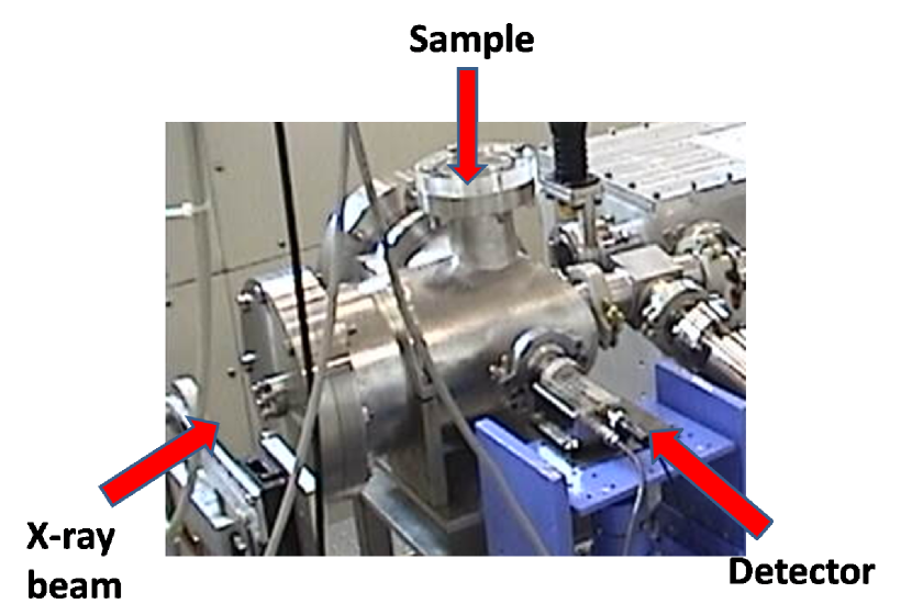
Figure 1: Photograph of the XRF experiment on lunar analogues under vacuum condition using synchrotron facility at RRCAT, Indore.

For the current experiment, the second crystal of DCM is detuned slightly to avoid higher order Bragg reflections from the DCM. The sample holder is placed at 45^∘ with respect to the incident beam direction. The monochromatic beam is allowed to pass through an ionization chamber for monitoring incident flux (I_o) reaching the sample. The fluorescent/scattered X-rays emitted from the sample are detected using a solid state Si PIN detector (XR-100CR - 160 eV at 5.9 keV; Amptek, Inc. USA) coupled to a digital pulse processor unit. The detector is placed in the horizontal plane perpendicular to the incident beam direction making a phase angle (angle between the incident beam, sample and detector) of ${\approx}$ 90^∘. The sample to detector distance is set to ${\approx}$ 10cm. A collimated mono-energetic X-ray beam of energy 8 keV and size ${\approx}$ 1mm ${\times}$ 1mm, is used for the sample excitation. All XRF measurements are done inside a vacuum chamber made out of stainless steel (SS-304) with pressure of ${\approx}$ 10^-2 mbar. Fig. (1) shows the photograph of the experimental arrangement at BL-16.

3 XRF spectral analysis

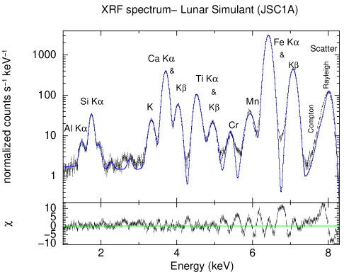
(a) XRF spectrum - Lunar simulant (JSC-1A) - Fit without trace elements

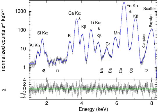
(b) XRF spectrum - Lunar simulant (JSC-1A) - Fit with trace elements

Figure 2: Best fit for the observed XRF spectra of JSC-1A showing the lines of major elements present in the sample (a) without trace elements (b) with trace elements marked vertically. Residuals of fit ie., difference between data and model represented in terms of standard deviation 1${\sigma}$ error bars (ref. delchi - XSPEC manual) are shown in the bottom panel of each figure. Data points are shown with error bars; line shows the spectral model fit to the data.

Observed XRF spectra of laboratory samples are analyzed using the X-ray spectral analysis package (XSPEC) (Arnaud,, 1966). The best spectral fit obtained for the samples JSC-1A and Sittampundi rock excited by an intense 8 keV mono-energetic beam are shown in Fig. (2 & 3). XRF lines of low Z elements like Al, Si, K are clearly visible in the spectrum which are modeled as Gaussian functions. X-ray signature of Mg is not seen in the spectrum of JSC-1A due to reduced efficiency of the detector at lower energies around 1 keV and also from a low probability to excite the relatively less abundant Mg by a 8 keV beam.

3.1 Spectral contamination and corrections

The observed XRF spectra also exhibit lines from elements which are not present in the samples as well as a continuum background emission. Reasons for these features seen in the spectrum and necessary corrections applied to derive the XRF line flux of the samples are discussed below:

• XRF lines of stainless steel arising from the vacuum chamber walls are clearly observed (for example K-${\alpha}$ of Cr @ 5.4 keV). This is probably due to the interaction of uncollimated scattered 8 keV beam with the walls of the vacuum chamber. As some of the elements in SS-304 are also present in the samples (ref. Fig. (2)), we have to estimate the contribution from SS-304. For this, we derived the XRF spectrum of SS-304 excited by an 8 keV beam using GEANT4 Monte Carlo simulation.

• Scattered continuum components of 8 keV incident beam: viz., Rayleigh (elastic) and Compton (inelastic) are also prominently seen in the observed spectra (ref. Fig.(2 &3)). Earlier experiments by Athiray et al., (2013) were performed with a lower intensity X-ray beam and hence did not reveal the presence of scattering components. To model the scattered components, using apriori composition, we simulated both elastic and inelastic scattered spectrum in GEANT4. We generated table models of the XRF spectrum of SS-304 and scatter component spectrum (elastic and inelastic) which are compatible for XSPEC analysis. Table models used in XSPEC are user defined models containing a grid of spectra and range of parameter values used in the model. While fitting the data, normalization of the differential flux is allowed to vary, retaining the the spectral profile.

• The samples also contain many trace elements (in ppm) which are mostly high Z (For JSC-1A ex. Ni, Zr, Sr, Ce, Ba etc.,). Many of these exhibit numerous L- lines which lie very close to/overlap XRF lines of major elements (for eg: L-lines of Ba lie close to Ti & Cr K-lines; Sr L-lines lie close to Si K-lines) in the samples. Presence of these trace element line features are clearly seen in the residuals in Fig. (2 (a)) when the spectrum is modeled only with major elemental lines, SS-304 lines and scatter components. Prominent trace element lines fitted with Gaussian functions in the XRF spectrum are shown in Fig. (2(b) & 3) (labeled vertically below the peaks).

Apart from these factors, a tiny fraction of contamination is expected due to scattering of these lines from perspex target holder. To account for possible contribution from unobserved trace elements and scattering from perspex, XRF line fluxes are considered to have a minimum uncertainty of 2%. Measured XRF line fluxes of the samples are derived after applying corrections for contamination. Figures 2 & 3 shows the best spectral fits to the samples after including all components (walls, trace elements, scattering). Flux-fractions are computed using eq.1 from the observed flux and fed to x2abundance along with the mono-energetic input spectrum.

$$FF_{i}=\frac{F_{i}}{{\sum}_{i=1}^{n}F_{i}}$$ (1)

where i run across all ‘n’ elements in the sample, $F_{i}$ - computed X-ray line flux of $i^{th}$ element, $FF_{i}$ - computed flux fraction of $i^{th}$ element. Elemental abundances are derived using x2abundance with computations performed for both cases ie., fitting with and without trace elements and the results are discussed below.

4 Laboratory experiment results

XRF lines of Mg, Na and O could not be seen in the spectrum of JSC-1A due to the reduced effective area of the detector below 1.2 keV. Hence the weight percentage values of these elements are fixed to values obtained from EDX measurements (2.6%, 1.5% and 52.7% ) respectively. Table 1 compares the elemental abundances of lunar simulant (JSC-1A) derived from x2abundance along with the measured values using EDX facility at ISAC. Column (3 & 4) gives the abundances derived for JSC-1A fitted with and without trace element contribution. Inclusion of trace elements in fitting can gives abundances which are closer to the true values.

For the analysis of Sittampundi sample, abundance of Oxygen is kept fixed as 57.0% (EDX measurement). Trace elements are fitted with Gaussians based on the residuals as a complete chemical characterization of these rocks are unavailable. Figure (4 (b)) compares major elemental abundances derived by x2abundance against the true abundances (EDX measurements) with 2${\sigma}$ residuals shown in the bottom panel. True elemental abundances agree well within 2${\sigma}$ errors of the derived values.

It should be noted that x2abundance does not demand any a priori information on the elemental weight percentages provided all the elements are observed in the spectrum (excluding Z $<$ 10). In this experiment, weight percentages of Mg and Na are obtained from EDX measurement, as they are not observed in the spectrum due to sensitivity of the detector at low X-ray energies. Experiments with Silicon Drift Detectors (SDD) can overcome this problem as it offers better quantum efficiency at low energies around ${\approx}$ 1 keV.

5 GEANT4 simulation and results

GEANT4 is a Monte Carlo based toolkit to simulate the interaction of particles through matter (Agostinelli et al.,, 2003). It incorporates various physics interactions, event tracking system, user-defined geometries, digitization etc., GEANT4 covers a wide range of energies of interaction (say 250eV to TeV energies) from optical to ${\gamma}$-rays and charged particles. It allows the user to define the incident beam, experimental geometry, sample composition and include necessary fundamental physics processes.

We have used GEANT4 (ver 9.4) with electromagnetic physics process including XRF and scattering (both elastic and inelastic). We defined the simulation geometry similar to that used in the laboratory, in order to cross validate x2abundance with laboratory experiments. We simulated XRF emission from a set of samples listed in Table 2. Simulated XRF line fluxes of all the elements are assumed to have Poisson errors. Flux-fractions are computed using eq.(1), which along with incident spectrum serve as input to x2abundance.

A comparison plot of derived abundance vs true abundance of all major elements for the sample JSC-1A simulated in GEANT4 experiment is shown in Fig. (5). It is evident from Fig. (5) that the abundances derived by x2abundance program matches well with the abundances for which GEANT4 simulation is performed. The deviation between the two is plotted as residuals in the bottom panel.

5.1 Cross-validation

We also tested the self-consistency of the inversion process by comparing the measured XRF spectrum with GEANT4 simulated spectrum which used the composition derived by x2abundance and convolved with instrument response. Steps involved in the cross-validation are shown in fig. (6). Elemental abundances of Sittampundi sample obtained from x2abundance are provided as input for GEANT4 XRF simulation. Fig. (7) shows the comparison of simulated flux-fractions plotted against the measured values. The plot also shows the best fit to the data where the slope tending to unity provides a good confidence in the x2abundance output. Deviation from the expected slope of unity could be due to unobserved trace elements not modeled in the spectrum.

6 Conclusion

Using the established FP method, we have developed an algorithm ‘x2abundance’ for remote sensing XRF observations. Major corrections required in the analysis of remote sensing observations viz., time and energy dependent excitation source, varying observation geometry, unknown composition, uncertain matrix effect are all incorporated in x2abundance. It is also to be noted that x2abundance provides the best suite elemental composition and its uncertainties. We have validated our approach using laboratory-based XRF experiments on metal alloys, lunar analogues and also using GEANT4 XRF simulations.

With this work, we complete the process of validation of x2abundance using laboratory XRF experiments on samples with atomic numbers (11 $<$ Z $<$ 30), which include all the major rock forming elements. We also report the validation of the same using simulated XRF spectra. It is shown that in all cases, the true abundances matches well within the uncertainty of our derived abundances.

However, as mentioned earlier, remote sensing measurements from planetary surfaces needs correction for the effect of surface roughness and grain size which are to be incorporated in x2abundance in order to approach the reality. As a future work, experiments are being planned to address the particle size effects along with sensitive measurements of low Z elements, whose characteristic X-ray peaks are around 1 keV.

7 Acknowledgments

The authors thank Dr. P. D. Gupta, Director RRCAT Indore for his encouragement and support in successfully conducting the experiment using the synchrotron facility. Our thanks to Shri. Ajith K Singh, Shri. Ajay Khooha, Shri. Vijendra Prasad and Shri. S. R. Garg of RRCAT Indore for their timely assistance. We also thank Ms. Uma Unnikrishnan for active discussions and help in GEANT4 simulation using user defined samples. We thank Prof. B.R.S. Babu and his team at the Dept., of Physics, University of Calicut for making pellets of the samples.

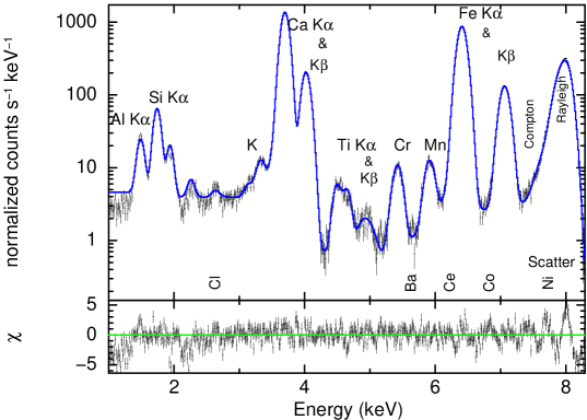
(a) XRF spectrum - Sittampundi Rock - Fit with trace elements

Figure 3: Best fit for the observed XRF spectra of Sittampundi rock sample (anorthositic composition) showing the lines of major elements present in the sample. Prominent trace elements and other components are marked. Residuals of fit represented in terms of sigma (1${\sigma}$) error bars (ref. delchi - XSPEC manual) are shown in the bottom panel of each figure.

(a) Lunar simulant (JSC-1A) - representing lunar mare

(b) Sittampundi sample - representing lunar highland

Figure 4: Comparison plot between the derived abundance (from x2abundance) and true abundance (EDX measurements) of laboratory lunar analogue samples. Residuals are plotted with 2${\sigma}$ confidence in the bottom panel

Table 1: Comparison of weight percentage (wt%) of major elements of JSC-1A as derived from x2abundance and EDX measurement values.

Element	Wt.% from	Wt.% from	Wt.% from
	EDX	x2abundance	x2abundance
	measurement	(with trace	(without trace
		elements$)$	elements$)$
Fe	7.5	7 ${\pm}$ 1	7 ${\pm}$ 1
Ti	1.1	1 $+$ 1	1 + 1
Ca	7.1	7 ${\pm}$ 1	7 ${\pm}$ 1
Si	19.5	18 ${\pm}$ 1	17 ${\pm}$ 1
Al	7.0	9 ${\pm}$ 1	10 ${\pm}$ 1

Figure 5: Comparison of abundance derived from simulated spectrum using x2abundance vs abundance assumed to create simulated spectrum in GEANT4 for the sample JSC-1A. Residuals are shown in the bottom panel.

Table 2: Samples used in GEANT4 simulations

S.No.	Name	Major elements
1	JSC-1A	Fe, Ti, Ca, Si, Al, Mg, Na, O
2	Sittampundi sample	Fe, Ca, Si, Al, Na, O

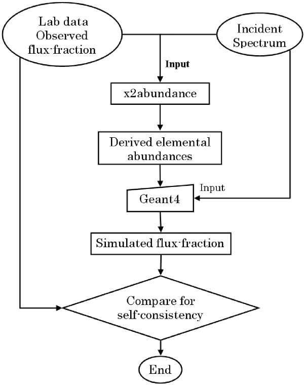
Figure 6: Steps involved in the cross-validation of x2abundance.

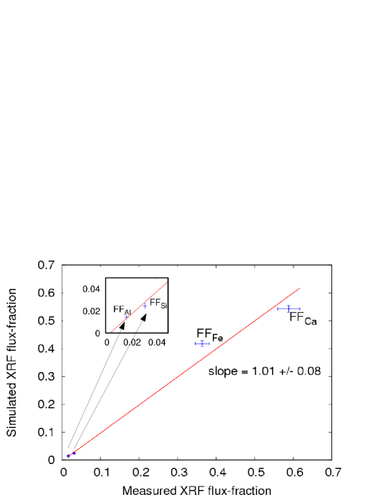
Figure 7: Comparison of XRF flux-fraction - measured vs simulated - Sittampundi sample

References

- Aarthy et al., (2009) Aarthy, R. S., et al., 2009. Spectral studies of Anorthosite and Meteorite. Proc. Lunar Planet. Sci. Conf. 40, 2216
- Agostinelli et al., (2003) Agostinelli, S. et al., 2003. GEANT4 - A simulation toolkit. Nucl. Instr. Meth. Res. A 506, 250-303.
- Anbazhagan et al., (2012) Anbazhagan, S. et al., 2012. Remote sensing study of Sittampundi Anorthosite complex, India. J. Indian Soc. Remote Sens.40, 145-153.
- Arnaud, (1966) Arnaud, K.A., 1966. XSPEC: The first ten years. ASP Conf. Ser. 101, 17–20.
- Athiray et al., (2013) Athiray, P. S., et al., 2013. Validation of methodology to derive elemental abundances from X-ray observations on Chandrayaan-1, Planet. Space Sci. 75, 188-194.
- Bhandari et al., (2005) Bhandari, N., 2005. Chandrayaan-1: science goals. Journal of Earth System Science 114, 701-709.
- Criss & Birks, (1968) Criss, J.W., Birks, L.S., 1968. Calculation methods for fluorescent X-ray Spectrometry: Empirical coefficients vs fundamental parameters. Anal. Chem. 40, 1080–1088.
- Fernandez, (1992) Fernandez, J.E., 1992. Rayleigh and Compton Scattering Contributions to X-ray Fluorescence Intensity, X-ray Spec. 21, 57-68.
- Grande et al., (2009) Grande, M., et al., 2009. The C1XS X-ray Spectrometer on Chandrayaan-1. Planet. Space Sci. 57, 717-724.
- Grieken & Markowicz (2002) Grieken, R.V., Markowicz, A., 2002. Handbook of X-ray Spectrometry. second ed. Marcel Dekker.
- Jenkins (1995) Ron Jenkins, Gould, R.W., Dale Gedcke, 1995. Quantitative X-ray Spectrometry. second ed. Marcel Dekker.
- Maruyama et al., (2008) Maruyama, Y., et al., 2008. Laboratory experiments of particle size effect in X-ray fluorescence and implications to remote X-ray spectrometry of lunar regolith surface. Ear. Planets Space, 60, 293-297.
- Nrnen et al., (2008) Nrnen, J., et al., 2008. Laboratory studies into the effect of regolith on planetary X-ray fluorescence spectroscopy. Icarus, 198, 408-419.
- Ray et al., (2010) Ray, C. S., et al., 2010. JSC-1A lunar soil simulant: Characterization, glass formation and selected glass properties. Jour. Non-crys. solids, 356, 2369-2374.
- Rousseau & Boivin, (1998) Rousseau, R., Boivin, J., 1998. The fundamental algorithm: A natural extension of Sherman equation. The Rigaku J. 15, 13–28.
- Tiwari et al., (2013) Tiwari, M. K., et al., 2013. A microfocus X-ray fluorescence beamline at Indus-2 synchrotron radiation facility. J. Synchrotron. Rad. 20, 386-389.
- Weider et al., (2012) Weider, S. Z., et al., 2012. The Chandrayaan-1 X-ray Spectrometer : First results. Planet. Space Sci. 60, 217-228.