Learning ambiguous functions by neural networks

Abstract

It is not, in general, possible to have access to all variables that determine the behavior of a system. Having identified a number of variables whose values can be accessed, there may still be hidden variables which influence the dynamics of the system. The result is model ambiguity in the sense that, for the same (or very similar) input values, different objective outputs should have been obtained. In addition, the degree of ambiguity may vary widely across the whole range of input values. Thus, to evaluate the accuracy of a model it is of utmost importance to create a method to obtain the degree of reliability of each output result. In this paper we present such a scheme composed of two coupled artificial neural networks: the first one being responsible for outputting the predicted value, whereas the other evaluates the reliability of the output, which is learned from the error values of the first one. As an illustration, the scheme is applied to a model for tracking slopes in a straw chamber and to a credit scoring model.

1 Introduction

When dealing with real-world problems, some degree of uncertainty can rarely be avoided. When modelling physical or social systems, either as a way for further understanding or as a guide for decision processes, dealing with uncertainty is a critical issue.

Uncertainty has been formalized in different ways leading to several uncertainty theories [1]. Here we will be concerned with uncertainty in the construction of models from observed data. In this context uncertainty may arise either from imprecision in the measurement of the observed variables or from the fact that the variables that can be measured do not provide a complete specification of the behavior of the system.

In the context of construction of models of physical phenomena by neural networks, the problem of learning from data with error bars has been addressed before by several authors (see for example [2] [3]). Here we will be mostly concerned not with imprecision in the input data but with the fact that the observed variables do not completely specify the output. In practice this situation is rather complex mainly because, in general, the uncertainty is not uniform throughout the parameter space. That is, there might be regions of the parameter space where the input variables provide an unambiguous answer and others where they are not sufficient to provide a precise answer. For example in credit scoring, which we will use here as an example, the ”no income, no job, no asset” situation is a clear sign of no credit reliability, but most other situations are not so clear-cut. Therefore it would be desirable to develop a method that, for each region of parameter space, provides the most probable outcome but at the same time tells us how reliable the result is.

The purpose of this paper is to develop such a system based on neural networks that learn in a supervised way. In short, the system consists of two coupled networks, one to learn the most probable output value for each set of inputs and the other to provide the expected error (or variance) of the result for that particular input. The system is formalized as the problem of learning random functions in the next section. Then we study two application examples, the first being the measurement of track angles by straw chambers in high-energy physics and the other a credit scoring model.

2 Learning the average and variance of random functions

The general setting which will be analyzed is the following:

The signal to be learned is a random function $y\left(\overset{\longrightarrow}{x}\right)$ with distribution $F_{\overset{\longrightarrow}{x}}\left(y\right)$. For simplicity we take $y$ to be a scalar and the index set $\left\{\overset{\longrightarrow}{x}\right\}$ to be vector-valued, $\overset{\longrightarrow}{x}\in\mathbb{R}^{i}$. Notice that we allow for different distribution functions at different points of the index set.

In the straw chamber example, to be discussed later, $\overset{\longrightarrow}{x}$ would be the set of delay times and $y$ the track angle. For the credit score example, $\overset{\longrightarrow}{x}$ would be the set of client parameters and $y$ the credit reliability.

In our learning system the $\overset{\longrightarrow}{x}$ values are inputs to a (feedforward) network with connection strengths $\left\{W\right\}$, the output being $f_{W}\left(\overset{\longrightarrow}{x}\right)$. The aim is to chose a set of connection strengths $\left\{W\right\}$ that annihilates the expectation value

$$\mathbb{E}\left\{\sum_{\left\{\overset{\longrightarrow}{x}\right\}}\left(f_{W}\left(\overset{\longrightarrow}{x}\right)-y\left(\overset{\longrightarrow}{x}\right)\right)^{2}\right\}=0$$

However, what, for example, the backpropagation algorithm does is to minimize $\mathbb{E}\left(f_{W}\left(\overset{\longrightarrow}{x}\right)-y\left(\overset{\longrightarrow}{x}\right)\right)^{2}$ for each realization of the random variable $\overset{\longrightarrow}{x}$. Let us fix $\overset{\longrightarrow}{x}$ and consider $f_{W}\left(\overset{\longrightarrow}{x}\right)$ evolving in learning time. That is, we are considering, in the learning process, the subprocess corresponding to the sampling of a particular fixed region of the index set. Then

$$f_{W}\left(\overset{\longrightarrow}{x},t+1\right) = f_{W}\left(\overset{\longrightarrow}{x},t\right)+\frac{\partial f_{W}}{\partial W}\bullet\Delta W$$

$$= f_{W}\left(\overset{\longrightarrow}{x},t\right)-\eta\frac{\partial f_{W}}{\partial W}\bullet\frac{\partial e}{\partial W}$$

$$= f_{W}\left(\overset{\longrightarrow}{x},t\right)-2\eta\frac{\partial f}{\partial W}\bullet\left(f_{W}\left(\overset{\longrightarrow}{x}\right)-y\left(\overset{\longrightarrow}{x}\right)\right)\frac{\partial f_{W}}{\partial W}$$

where $\Delta W=-\eta\frac{\partial e}{\partial W}$, $\eta$ being the learning rate and $e=\left(f_{W}\left(\overset{\longrightarrow}{x}\right)-y\left(\overset{\longrightarrow}{x}\right)\right)^{2}$ the error function.

If the learning rate $\eta$ is sufficiently small for the learning time scale to be much smaller than the sampling rate of the $y\left(\overset{\longrightarrow}{x}\right)$ random variable, the last equality may be approximated by

$$f_{W}\left(\overset{\longrightarrow}{x},t+1\right)=f_{W}\left(\overset{\longrightarrow}{x},t\right)-2\eta\frac{\partial f}{\partial W}\bullet\left(f_{W}\left(\overset{\longrightarrow}{x}\right)-\overline{{y}}\left(\overset{\longrightarrow}{x}\right)\right)\frac{\partial f_{W}}{\partial W}$$

$\overline{{y}}\left(\overset{\longrightarrow}{x}\right)$ denoting the average value of the random variable $y$ at the argument $\overset{\longrightarrow}{x}$. Then a fixed point is obtained for

$$f_{W}\left(\overset{\longrightarrow}{x}\right)=\overset{-}{y}\left(\overset{\longrightarrow}{x}\right)$$

That is, $f_{W}\left(\overset{\longrightarrow}{x}\right)$ tends to the average value of the random variable $y$ at $\overset{\longrightarrow}{x}$.

Similarly if a second network (with output $g_{W^{\prime}}\left(\overset{\longrightarrow}{x}\right)$) and the same input $\overset{\longrightarrow}{x}$ is constructed according to the learning law

$$g_{W^{\prime}}\left(\overset{\longrightarrow}{x},t+1\right)=g_{W^{\prime}}\left(\overset{\longrightarrow}{x},t\right)+\frac{\partial g_{W^{\prime}}}{\partial W^{\prime}}\bullet\Delta W^{\prime}$$

with error function

$$e^{\prime}=\left(g_{W^{\prime}}\left(\overset{\longrightarrow}{x}\right)-\left(f_{W}\left(\overset{\longrightarrow}{x}\right)-y\left(\overset{\longrightarrow}{x}\right)\right)^{2}\right)^{2}$$

and $\Delta W^{\prime}=-\eta^{\prime}\frac{\partial e^{\prime}}{\partial W^{\prime}}$, then

$$g_{W^{\prime}}\left(\overset{\longrightarrow}{x},t+1\right)=g_{W^{\prime}}\left(\overset{\longrightarrow}{x},t\right)-2\eta^{\prime}\frac{\partial g_{W^{\prime}}}{\partial W^{\prime}}\bullet\frac{\partial g_{W^{\prime}}}{\partial W^{\prime}}\left(g_{W^{\prime}}\left(\overset{\longrightarrow}{x}\right)-\left(f_{W}\left(\overset{\longrightarrow}{x}\right)-y\left(\overset{\longrightarrow}{x}\right)\right)^{2}\right)$$

and, under the same assumptions as before concerning the smallness of learning rates, $g_{W^{\prime}}\left(\overset{\longrightarrow}{x}\right)$ has the fixed point

$$g_{W^{\prime}}\left(\overset{\longrightarrow}{x}\right)=\overline{{\left(y\left(\overset{\longrightarrow}{x}\right)-\overline{{y}}\left(\overset{\longrightarrow}{x}\right)\right)^{2}}}$$

In conclusion: the first network reproduces the average value of the random function $y$ for each input $\overset{\longrightarrow}{x}$ and the second one, receiving as data the errors of the first, reproduces the variance of the function at $\overset{\longrightarrow}{x}$. Instead of the variance, the second network might as well be programed to learn the expected value of the absolute error $\mathbb{E}\left|y\left(\overset{\longrightarrow}{x}\right)-\overset{-}{y}\left(\overset{\longrightarrow}{x}\right)\right|$. Actually, for numerical convenience, we will use this alternative in the examples of the next section (Fig.3).

In practice the training of the second network should start after the first one because, before the first one becomes to converge, its errors are not representative of the fluctuations of the random function. In general it seems reasonable to have $\eta^{\prime}\left(t\right)<\eta\left(t\right)$with $\eta\left(t\right)$decreasing in time towards a small fixed value $\neq 0$.

3 Examples:

3.1 Measuring track angles by straw chambers

One of the first applications of neural networks to the processing of high-energy physics data was the work by Denby, Lessner and Lindsey [4] on the slopes of particle tracks in straw tube drift chambers. In a straw chamber (Fig.1) each wire receives a signal delayed by a time proportional to the distance of closest approach of the particle to the wire.

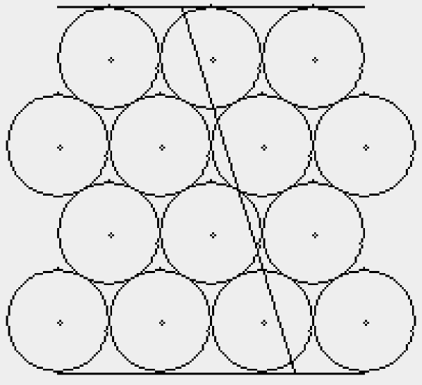
Figure 1: A particle track through a straw chamber. The input values to the neural networks are the delay times, proportional to the distances of the particle to the wires

The neural network receives these times as inputs $\left\{\overset{\longrightarrow}{x}\right\}$, with as many inputs as the number of wires and, for the training, the track angle $y\left(\overset{\longrightarrow}{x}\right)$is the objective function. The half cell shift of alternate layers in the straw chamber solves some of the left-right ambiguities but this ambiguity still remains for many directions (Fig.2).

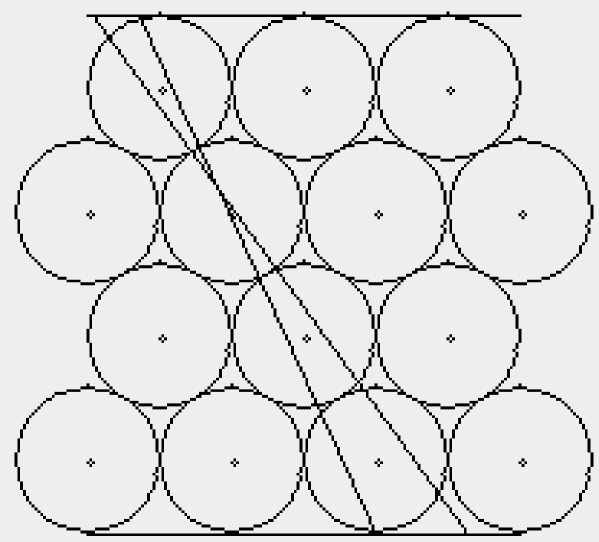
Figure 2: An example with two different beam track angles generating the same input signal

The authors of [4] required the training and test events to pass through at least four straws to avoid edge effects. Nevertheless they consistently find large non-Gaussian error tails when testing the trained network. The authors have not separated the contribution to the tails coming from the ambiguities from those arising from eventual inadequacies on training or network architecture. We have repeated the simulations and our results essentially reproduce those of [4], showing that the non-Gaussian tails do indeed originate from the left-right ambiguities. If edge effects are allowed for, including in the training set events that pass through less than four straws, the degree of ambiguity and the tails increase even further.

This example is therefore a typical example of the situation described in the introduction, where some regions of the input data correspond to a unique event but others have an ambiguous identification. As the example shows it is not easy to separate the ambiguous regions from the non-ambiguous ones because they are mixed all over parameter space. It is therefore important to have a system that not only provides an answer but also states how reliable that answer is.

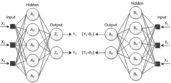
Figure 3: A two-network system that, given inputs $X_{i}$ and objective values $\theta_{k}$, learns the average values $\overline{Y_{k}}\left(X_{i}\right)$ and average errors $\overline{\left|Y_{k}-\theta_{k}\right|}$for each set $\left\{X_{i}\right\}$of input values

We have applied to this example the two-network scheme (Fig.3) described before. Both networks have the same architecture and train using the same exact input data, the first one (at left in Fig.3) with the objective track angles and the second (at right in Fig.3) with the absolute value of the errors of the first. To avoid big fluctuations in training convergence, the second network starts learning after the first has stabilized and finished training. Both networks have a feed-forward network architecture with three neuron layers: input, hidden and output. They both train using a supervised backpropagation algorithm. The neuron activation function is the logistic sigmoid.

For the results presented here we use 14 input neurons (representing the drift times in each straw), 25 hidden neurons and an output neuron for the slope of each track. We use Monte Carlo generated data coded as follows: If the track does not meet the straw the input value is zero and if the track crosses the straw the input value is the difference between the straw radius and the distance to the wire in the center of the straw. The output is the angle in degrees of the track slope. A training sample of $25000$ simulated tracks was generated which trained for $12.5\times 10^{6}$ iterations. After training, the performance of the network was tested using a new set of $5000$ independent tracks. Fig.4 shows a plot of the first network errors obtained with the test set. The distribution does present large non-Gaussian tails because of the left-right ambiguity.

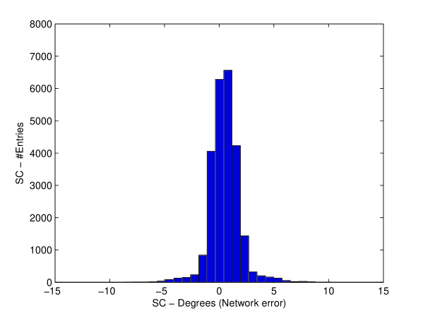
Figure 4: Error distribution in the first network (straw chamber data)

Fig.5 compares the actual error of the first network with the uncertainty predicted by the second. One sees that the largest actual errors do indeed correspond to good uncertainty predictions by the second network. Of course in a few cases large uncertainty is predicted when the actual error is small. It only means that particular result is unreliable in the sense that it was by chance that it fell in the middle of the error bar interval.

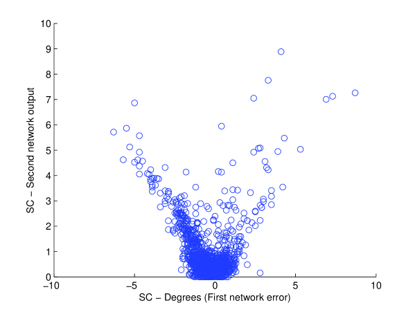
Figure 5: Comparison of the actual error of the first network and the estimated uncertainty predicted by the second network (straw chamber data)

Now that we are equipped with a system that predicts both an angle and its probable uncertainty, it makes sense to state that the result of a measurement is $\theta\pm\Delta_{ann}$, $\theta$ being the output of the first network and $\Delta_{ann}$the output of the second. In this sense we will count an output as an error only when the objective value is outside the error bars. The effective error will be the distance of the objective value to the boundary of the error bars. Fig.6 plots the effective error for a sample of $1000$ tracks. Comparison with Fig.4 shows how the reliability of the system is improved, because each time an output value is obtained one has a good estimate of how accurate it is.

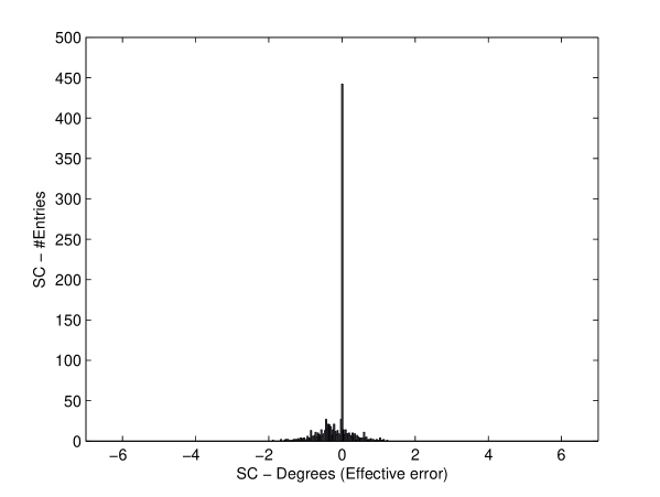
Figure 6: Effective error (straw chamber data)

3.2 A credit scoring model

Defaulting on loans has recently increased, promoting the search for accurate techniques of credit evaluation by financial institutions. Credit scoring is a quantitative method, based on credit report information that helps lenders in the credit granting decision. The objective is to categorize credit applicants into two separate classes: the ”good credit” class, that is, the one likely to repay loans on time and the ”bad credit” class to which credit should be denied, due to a high probability of defaulting. For a more detailed understanding of credit scoring models, with and without neural networks, we refer to [5] [6] [7] [8].

Here we have developed a credit scoring model based on the two-network scheme discussed before. Because complete information on the credit applicants is impossible to obtain and human behavior is dependent on so many factors, credit scoring is also a typical example of a situation where one is trying to predict an outcome based on incomplete information.

For the purpose of an open illustration of our system we use here a publicly available credit data of anonymous clients, downloaded from UCI Irvine Machine [9]. It is composed of $1000$ cases, one per applicant, of which $700$ cases correspond to creditworthy applicants and $300$ cases correspond to applicants which were later found to be in the bad credit class. Each instance corresponds to $24$ attributes (e.g., loan amount, credit history, employment status, personal information, etc.) with the corresponding credit status of each applicant coded as good ($1$) or bad ($0$). Inspecting the database, it is clear that some apparently good attributes correspond, in the end, to bad credit performance and conversely, putting into evidence the incomplete information nature of the problem.

For our system the attributes are numerically coded and we use a neural network architecture with $24$ input neurons (representing the $24$ numerical attributes), $14$ hidden neurons and an output neuron indicating good or bad credit. The network trained $1000000$ times. To ensure that the network learns evenly, we randomly alternate between good and bad applicants instances. After training, the performance of the network was tested. Fig.7 shows a plot of the errors of the first network after training. Although, in general, the network provides good estimations, there are several customers classified as good when they are bad and vice-versa. In fact, there are some extremely incorrect network predictions, as can easily been perceived by the bins at the two ends of the histogram. These bins clearly reveal lack of information in the dataset.

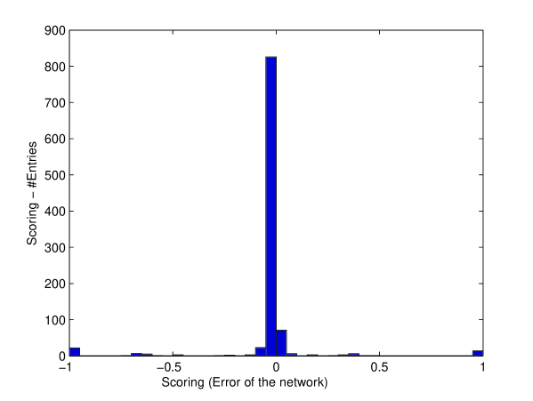
Figure 7: Error distribution in the first network (credit scoring)

As in the previous example, Fig.8 shows the comparison of the errors in the first network with the estimated uncertainty obtained by the second network and Fig.9 shows the effective error distribution. Similarly to the previous straw chamber example, one obtains good uncertainty predictions by the second network. The second network wrongly classified very few cases: only two occurrences with no actual errors were predicted having maximum uncertainty and only three critical errors were unsuccessfully predicted without uncertainty.

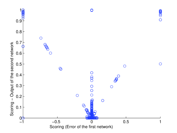
Figure 8: Comparison of the actual error of the first network and the estimated uncertainty predicted by the second network (credit scoring)

Looking at the effective error distribution plot, it is easy to confirm the refinement in the degree of certainty in each estimation. Nevertheless, there still are a very few occurrences of estimations outside the error bar interval. Complexity of the human behavior?

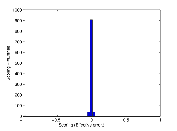
Figure 9: Effective error (credit scoring)

3.3 Conclusions

The goal of this research was to develop a computational scheme with the ability to evaluate the degree of reliability of predictive models. Two application examples were studied, the first one being the measurement of track angles by straw chambers in high-energy physics and the other a credit scoring model. Both examples use data with incomplete information. A two-network system is used which, although not perfect, greatly improves the reliability check of the predicted results.

References

- [1] G. J. Klir; Developments in uncertainty-based information, Advances in Computers 36 (1993) 255-332.
- [2] K. A. Gernoth and J. W. Clark; A modified backpropagation algorithm for training neural networks on data with error bars, Computer Physics Commun. 88 (1995) 1-22.
- [3] B. Gabrys and A. Bargiela; Neural network based decision support in presence of uncertainties, ASCE J. of Water Resources Planning and Management 125 (1999) 272-280.
- [4] B. Denby, E. Lessner and C. S. Lindsey; Test of track segment and vertex finding with neural networks, Proc. 1990 Conf. on Computing in High Energy Physics, Sante Fe, NM. 1990, AIP Conf Proc. 209, 211.
- [5] D. Lando; Credit Risk Modeling, Princeton U. P. 2004.
- [6] T. Van Gestel and B. Baesens; Credit Risk Management: Basic concepts: Financial risk components, Rating analysis, models, economic and regulatory capital, Oxford, 2009.
- [7] E. M. Lewis; An Introduction to Credit Scoring, Fair, Isaac and Co., San Rafael 1992.
- [8] D. West; Neural network credit scoring models, Computers and Operations Research 27 (2000) 1131-1152.
- [9] UCI Machine Learning Repository; URL http://archive.ics.uci.edu/ml/