Compression of animated 3D models using HO-SVD

Abstract

This work presents an analysis of Higher Order Singular Value Decomposition (HO-SVD) applied to lossy compression of 3D mesh animations. We describe strategies for choosing a number of preserved spatial and temporal components after tensor decomposition. Compression error is measured using three metrics (MSE, Hausdorff, MSDM). Results are compared with a method based on Principal Component Analysis (PCA) and presented on a set of animations with typical mesh deformations.

1 Introduction

The goal of this paper is to provide an analysis of Higher Order Singular Value Decomposition [DLDMV00] (HO-SVD) applied to lossy compression of 3D mesh animations. The paper includes an estimation of compression quality using three error metrics, a discussion about selection of parameters and a comparison with a method based on Principal Component Analysis (PCA). We provide a simple, heuristic method for HO-SVD parameter selection. Results are presented using a diverse set of well-known mesh animations, representing several common cases of 3D shape deformation.

HO-SVD is a multi-linear generalization of Singular Value Decomposition. It has been shown (e.g. in [IU05]) that HO-SVD is an efficient method for dimensionality reduction of data represented as tensors, also called N-way arrays. While consecutive frames of a 3D animation can naturally be represented as a 3-mode tensor (a data cube), by stacking arrays of their vertices, application of HO-SVD for such data requires additional considerations.

When using PCA-based compression, only a single parameter related to the number of preserved principal components is needed. Usually (e.g. [AM00], [SSK05]), dimensionality reduction is applied to animation frames, reducing their number to a sequence of significant key-frames. On the contrary, HO-SVD-based compression allows for multidimensional reduction of the data tensor, so it is possible to achieve the desired compression ratio with multiple sets of parameters. In our experiment we truncated the number of mode-$1$ (mesh vertices) and mode-$3$ (animation frames) components obtained through tensor decomposition. Reduction of mode-$2$ components (3D coordinates of vertices) is not advised since it results in a significant loss of information and low quality of reconstructed data. We assume that the best set of parameters for a desired compression ratio is the one introducing the lowest distortion of reconstructed objects.

For estimation of the quality of lossy compression we used three metrics. The Mean Squared Error (MSE) and the Hausdorff distance are both widely used for measuring 3D mesh distortions. Additionally, we decided to include a third metric, the Mesh Structural Distortion Measure (MSDM), since according to [LDD^∗06], it correlates well with human perception of errors in 3D data. Fig.1 presents an example of a distortion, resulting from a reconstruction of an animation compressed with HO-SVD.

The article is organised as follows. In the two following subsections, the related work and HO-SVD decomposition are presented. Definitions and methodology of our experiments are presented in Section 2. Obtained results can be found in Section 3, while their summary along with our comments are presented in Section 4.

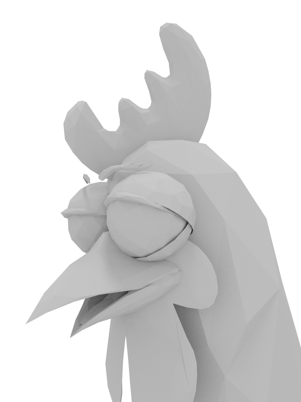
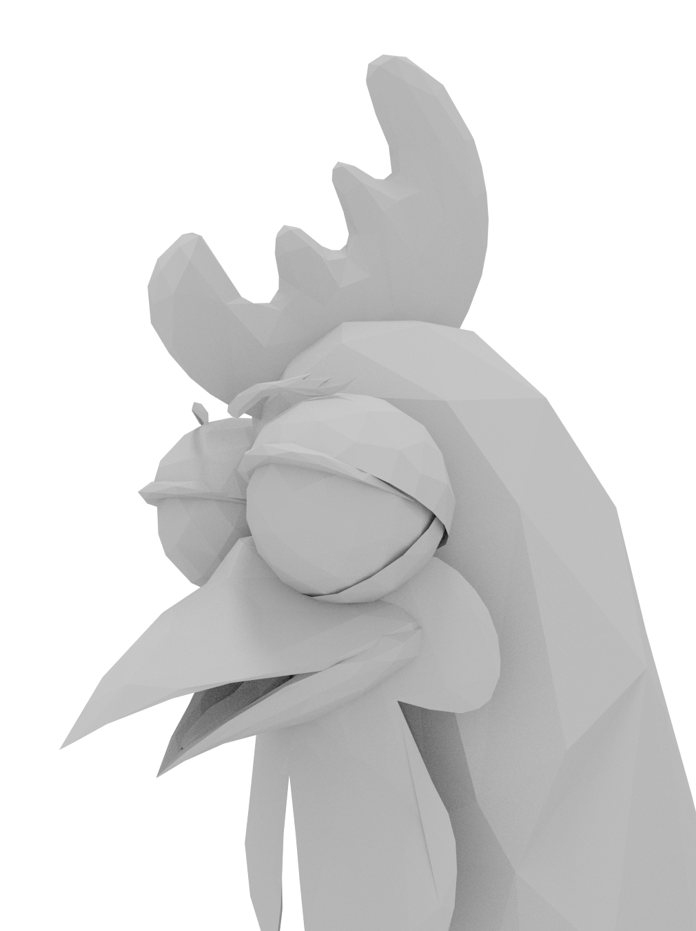
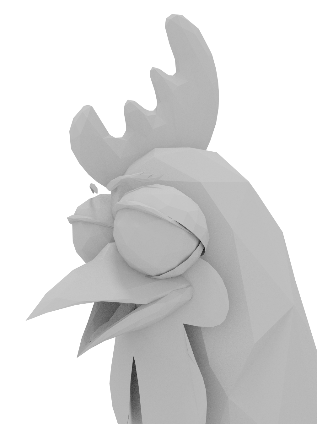
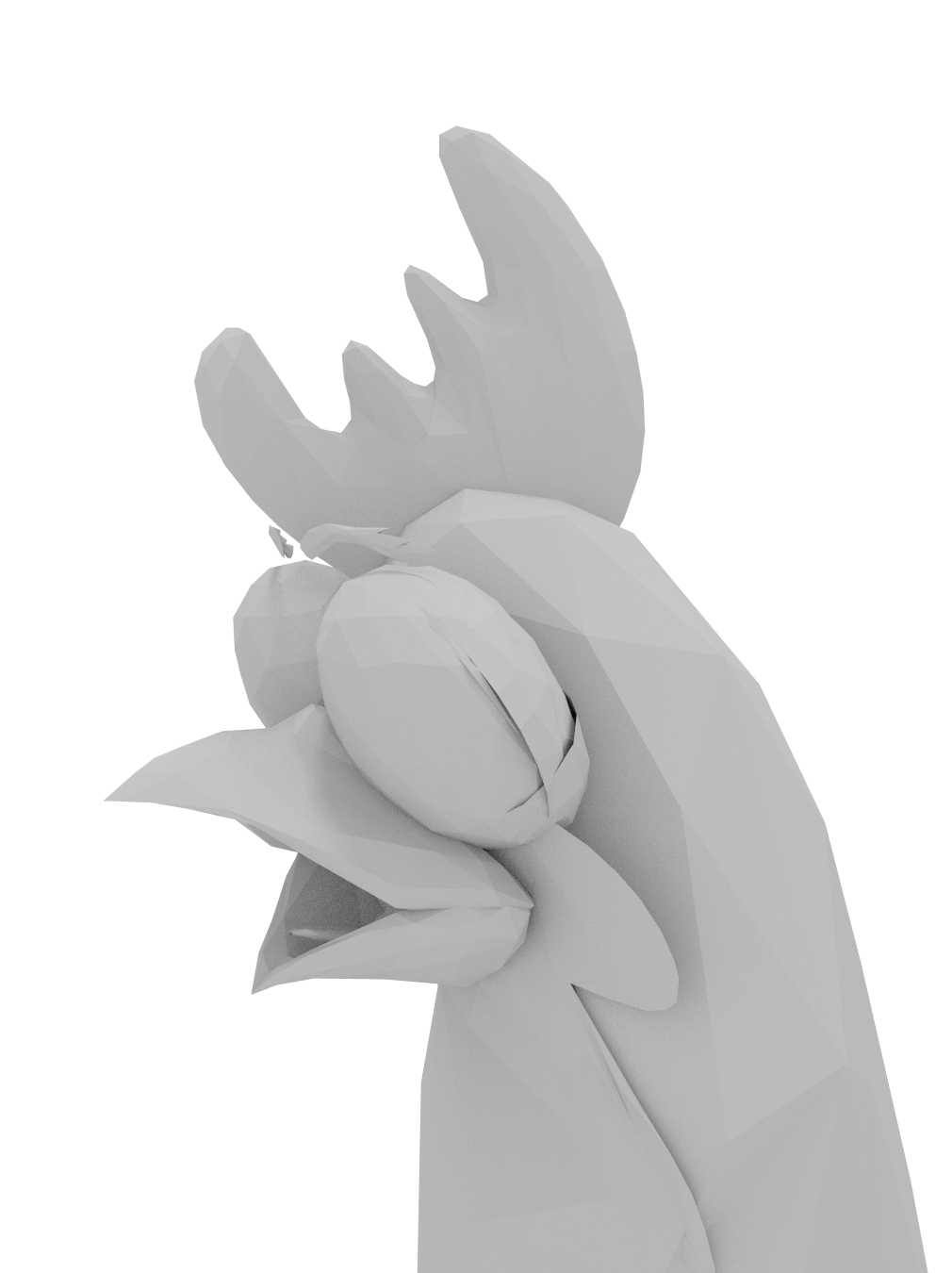
Figure 1: A fragment of a reconstructed animation sequence for Chicken animation. Panel (a) presents an original model, in further panels the data tensor is compressed to (b): 5.1%, (c): 2.1%, and (d): 1.1% of its original size.

1.1 Related work

Due to their amount, data generated by using 3D scanners or animation software require effective compression methods for their storage, transmission, and processing. An in-depth survey of 3D mesh compression techniques along with formulation of related problems is provided in [PKK05]. Various approaches for 3D data modelling, e.g. using efficient octree coding and attribute quantization [HPKG08] or combining surface and probabilistic approximation [GS13] are used to effectively store and reproduce digitized objects.

Frame-based Animated Mesh Compression was recently promoted within the MPEG-4 standard as Amendement 2 to part 16 (AFX, Animation Framework eXtension) and is described in [MZP08]. A representation of animation sequences using Principal Component Analysis (PCA) was introduced in [AM00]. This approach was further refined in [SSK05] where authors performed motion clustering on an animation and applied PCA to its subsegments, substantially improving the reconstruction quality. A summary of PCA-based applications to 3D animation compression, along with a broad analysis of related topics is provided in [AS09].

Higher Order Singular Value Decomposition (HO-SVD) may be treated as a natural extension of PCA for high-dimensional data. A survey of tensor properties as well as the description of higher-order tensor decomposition is provided in [KB09]. An application of HO-SVD to face recognition is presented in [WA03]. The authors used a data tensor consisting of a classification index, along with subspaces corresponding to human facial features and expressions. After tensor decomposition, face recognition was performed using the $k$-NN classifier.

An interesting representation of 3D animation using HO-SVD is provided in [ASK^∗12], with applications including dimensionality reduction, denoising and gap filling. HO-SVD was also used in [MK07] for level-of-detail reduction in animations of human crowds, where encoded motion tensors are represented with a number of components dependent on the distance from the camera.

1.2 Higher Order Singular Value Decomposition

Higher Order Singular Value Decomposition, also called Tucker decomposition, is a generalisation of SVD from matrices to tensors (N-way arrays). In this section we recall basic facts about tensors and HO-SVD. We follow conventions presented in [KB09].

To describe this decomposition, first we will recall basic notions regarding operations on tensors. Let a tensor

$$\mathcal{T}=\{t_{i_{1},i_{2},\ldots,i_{n}}\}_{i_{1},i_{2},\ldots,i_{n}=0}^{I_{1}-1,I_{2}-1,\ldots,I_{N}-1}\in\mathbb{R}^{I_{1},I_{2},\ldots,I_{N}}$$ (1)

be given — we say that this tensor has $n$ modes. Each of the indices corresponds to one of the modes i.e. $i_{l}$ to mode $l$.

By multiplication of tensor $\mathcal{T}$ by matrix $\mathbf{U}=\{u_{i_{l}d}\}_{i_{l},d=0}^{I_{l}-1,D}\in\mathbb{R}^{I_{l},D}$ in mode $l$ we define tensor $\mathcal{T}^{\prime}\in\mathbb{R}^{I_{1},\ldots,I_{l-1},D,I_{l+1},\ldots,I_{N}}$, such that:

$$\mathcal{T}^{\prime}=(\mathcal{T}\times_{l}\mathbf{U})_{i_{1}\ldots i_{l-1}d\,i_{l+1}\ldots i_{N}}=\sum_{{i}_{l}=0}^{I_{l}-1}t_{i_{1}i_{2}\ldots{i}_{l}\ldots i_{N}}u_{i_{l}d}.$$ (2)

By unfolding tensor $\mathcal{T}$ in mode $l$ we define matrix $\mathbf{T}_{(l)}$ such that

$$(\mathbf{T}_{(l)})_{i,j}=t_{i_{1}\ldots i_{l-1}j\,i_{l+1}\ldots i_{N}},$$ (3)

where

$$i=1+\sum_{\begin{subarray}{c}k=1\\ l\neq l\end{subarray}}^{N}J_{k}\text{ \ and \ }J_{k}=\prod_{\begin{subarray}{c}m=1\\ m\neq l\end{subarray}}^{k-1}I_{m}.$$

Given tensor $\mathcal{T}$, defined as in Eq. (1), a new sub-tensor $\mathcal{T}_{{i}_{n}=\alpha}$ can be created according to the equation with the following elements:

$$\mathcal{T}_{{i}_{l}=\alpha}=\{t_{i_{1}i_{2}\ldots i_{l-1}i_{l+1}\ldots i_{n}}\}_{i_{1}=0,i_{2}=0,\ldots,i_{l}=\alpha,\ldots,i_{n}=0}^{I_{1}-1,I_{2}-1,\ldots,\alpha,\ldots,I_{N}-1}\in\mathbb{R}^{I_{1},I_{2},\ldots,1,\ldots,I_{N}}.$$ (4)

The scalar product $\langle\mathcal{A},\mathcal{B}\rangle$ of tensors $\mathcal{A},\mathcal{B}\in\mathbb{R}^{I_{1},I_{2},\ldots,I_{N}}$ is defined as

$$\langle\mathcal{A},\mathcal{B}\rangle=\sum\limits_{i_{1}=0}^{I_{1}-1}\sum\limits_{i_{2}=0}^{I_{2}-1}\ldots\sum\limits_{i_{N}=0}^{I_{N}-1}b_{i_{1},i_{2},\ldots,i_{n}}a_{i_{1},i_{2},\ldots,i_{n}}.$$ (5)

We say that if scalar product of tensors equals 0, then they are orthogonal.

The Frobenius norm of tensor $\mathcal{T}$ is given by

$$||\mathcal{T}||=\sqrt{\langle\mathcal{T},\mathcal{T}\rangle}.$$ (6)

Given tensor $\mathcal{T}$, in order to find its HO-SVD, in the form of the so called Tucker operator $\llbracket\mathcal{C};\mathbf{U}^{(1)},\ldots,\mathbf{U}^{(N)}\rrbracket$, such that $\mathcal{C}\in\mathbb{R}^{I_{1},\ldots,I_{N}}$ and $\mathbf{U}^{(k)}\in\mathbb{R}^{I_{k}\times I_{k}}$ are orthogonal matrices, Algorithm 1 can be used.

Input: Data Tensor $\mathcal{T}$

Output: Tucker operator $\llbracket C;\mathbf{U}^{(1)},\ldots,\mathbf{U}^{(N)}\rrbracket$

for $k\in\{1,\ldots,N\}$ do

       $\mathbf{U}^{(k)}=\text{ left singular vectors of }T_{(k)}\text{ in unfolding }k$;

      

end for

$C=\mathcal{T}\times_{1}\mathbf{U}^{(1)T}\times_{2}\mathbf{U}^{(2)T}\ldots\times_{N}\mathbf{U}^{(N)T}$;

return $\llbracket C;\mathbf{U}^{(1)},\ldots,\mathbf{U}^{(N)}\rrbracket$;

Algorithm 1 HO-SVD algorithm

Tensor $\mathcal{C}$ is called the core tensor and has the following useful properties.

• Reconstruction:

  $$\mathcal{T}=\mathcal{C}\times_{1}\mathbf{U}^{(1)}\times_{2}\mathbf{U}^{(2)}\times_{3}\ldots\times_{N}\mathbf{U}^{(N)},$$ (7)

  where $\mathbf{U}^{(i)}$ are orthogonal matrices;

• Orthogonality:

  $$\langle\mathcal{C}_{{i}_{l}=\alpha},\mathcal{C}_{{i}_{l}=\beta}\rangle=0$$ (8)

  for all possible values of $l$, $\alpha$ and $\beta$, such that $\alpha\neq\beta$;

• Order of sub-tensor norms:

  $$||\mathcal{C}_{{i}_{n}=1}||\leq||\mathcal{C}_{{i}_{n}=2}||\leq\ldots\leq||\mathcal{C}_{{i}_{n}=I_{n}}||$$ (9)

  for all $n$.

Therefore, informally, one can say that larger values of a core tensor are denoted by low values of indices. This property is the basis for the development of compression algorithms based on HO-SVD.

Formally

$$\mathcal{\tilde{T}}=\tilde{\mathcal{C}}\times_{1}\tilde{\mathbf{U}}^{(1)}\times_{2}\tilde{\mathbf{U}}^{(2)}\times_{3}\ldots\times_{N}\tilde{\mathbf{U}}^{(N)},$$ (10)

where

$$\mathcal{\tilde{C}}=\{c_{i_{1},i_{2},\ldots,i_{n}}\}_{i_{1},i_{2},\ldots,i_{n}=0}^{R_{1}-1,R_{2}-1,\ldots,R_{N}-1}\in\mathbb{R}^{R_{1},R_{2},\ldots,R_{N}}$$ (11)

is a truncated tensor in such a way that in each mode $l$ indices span from 0 to $R_{l}-1\leq I_{l}-1$ and $\tilde{\mathbf{U}}^{(l)}\in\mathbb{R}^{R_{l}\times I_{l}}$ matrices whose columns are orthonormal and rows form orthonormal basis in respective vector spaces. A visualization of $3$-mode truncated tensor is provided in Fig. 2

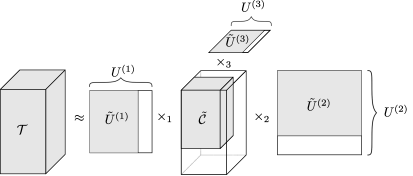
Figure 2: Truncated HO-SVD decomposition of tensor $\mathcal{T}$. Its approximation, tensor $\tilde{\mathcal{T}}$, can be reconstructed from a truncated tucker operator $\llbracket\tilde{C};{\tilde{\mathbf{U}}^{(1)},\tilde{\mathbf{U}}^{(2)},\tilde{\mathbf{U}}^{(3)}}\rrbracket$. The visualization is inspired by [KB09].

Given $(R_{l})_{l=1}^{N}$ one can form tensor $\mathcal{\tilde{T}}$ that approximates tensor $\mathcal{T}$ in the sense of their euclidean distance $||\mathcal{\tilde{T}}-\mathcal{T}||$. This approximation can be exploited to form lossy compression algorithms of signals that are indexed by more than two indices. It should by noted that the choice of $(R_{l})_{l=1}^{N}$ in a given application is non-obvious and depends on the properties of processed signals.

2 Method

Our experiments aim to assess the effectiveness of HO-SVD for compression of 3D animations. Additionally we want to present a clear strategy for choosing the proportion of preserved spatial and temporal components in order to maintain good quality of reconstructed data. We will present results using multiple error metrics and compare them to a method based on PCA.

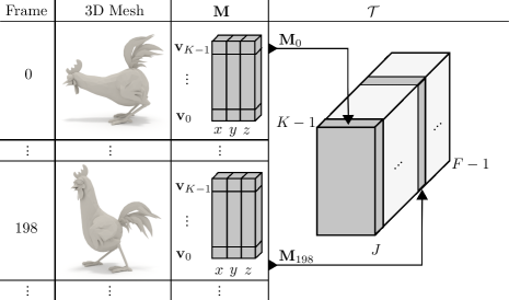
Figure 3: Visualization of data tensor $\mathcal{T}$. It is formed by stacking vertices of meshes, corresponding to $F$ animation frames, represented as $K\times J$ arrays.

2.1 Input data

Three-dimensional mesh will be treated as a $K\times J$ matrix $\mathbf{M}$, with mesh vertices $\mathbf{v}_{i}\in\mathbb{R}^{J},i\in\{0,\dots,K-1\}$ as rows, together with a set of edges $\mathfrak{G}$. We denote $J=3$ as a number of spatial dimensions. An animation consists of $F$ successive frames enumerated with $k$, each containing a mesh $\mathbf{M}_{k},k\in\{0,\dots,F-1\}$, with the same topology, but different coordinates of vertices. Therefore, input data can form tensor $\mathcal{T}=t_{i,j,k}\in\mathbb{R}^{K\times J\times F}$ while meshes $\mathbf{M}_{k}$, following the notation in [KB09], form frontal slices $\mathcal{T}_{::i}$. Tensor visualization is presented in Fig. 3. A pair $(\mathcal{T},\mathfrak{G})$ contains all available information about the animation. We apply compression only to $\mathcal{T}$, a set of edges $\mathfrak{G}$ is used only for data visualization.

2.2 Compression testing procedure

Algorithm 2 presents stages of the procedure aimed at calculating the quality of mesh reconstruction.

Input: Data Tensor $\mathcal{T}$, Compression rate $CR$, Quality metric $d$

Output: Quality of $\mathcal{T}^{\prime}$

/* $\mathcal{X}$ is a normalised tensor */

/* $\mathfrak{R}$ is a sequence of homography matrices */

$\mathcal{X}$, $\mathfrak{R}$ = Rigid Motion Estimation($\mathcal{T}$);

/* $\llbracket C;\mathbf{U}^{(1)},\mathbf{U}^{(2)},\mathbf{U}^{(3)}\rrbracket$ is the Tucker operator */

$\llbracket C;\mathbf{U}^{(1)},\textbf{U}^{(2)},\textbf{U}^{(3)}\rrbracket$ = HOSVD Decomposition(X);

/* $VTF$ is a scalar of Vertex-to-Frame ratio */

$VTF$ = Estimate VTF($\llbracket C;\mathbf{U}^{(1)},\mathbf{U}^{(2)},\mathbf{U}^{(3)}\rrbracket$, $CR$);

$\llbracket\tilde{C};{\tilde{\mathbf{U}}^{(1)},\tilde{\mathbf{U}}^{(2)},\tilde{\mathbf{U}}^{(3)}}\rrbracket$ = Truncate(($\llbracket C;{\mathbf{U}^{(1)},\mathbf{U}^{(2)},\mathbf{U}^{(3)}}\rrbracket$)

$\tilde{\mathcal{T}}$ = Reconstruct($\llbracket\tilde{C};{\tilde{\mathbf{U}}^{(1)},\tilde{\mathbf{U}}^{(2)},\tilde{\mathbf{U}}^{(3)}}\rrbracket$, $VTF$, $CR$, $\mathfrak{R}$);

return $\mathrm{d}(\mathcal{T},\tilde{\mathcal{T}})$;

Algorithm 2 A procedure for estimating the quality of HO-SVD compression for 3D animation. Similar procedure is performed for PCA.

The algorithm consist of the following steps:

1. Rigid motion estimation:
   The rigid motion of a mesh over the whole animation is estimated and subtracted from consecutive frames. Sequence $\mathfrak{R}=(\mathbf{R}_{i})_{i=0}^{F-1}$ is created where $\mathbf{R}_{i}$ is a matrix of an affine transformation between frame $i$ and $0$. Consecutive frames are translated into the coordinates of the first frame, forming normalised data tensor $\mathcal{X}:\forall_{i}\mathcal{X}_{::i}=\mathcal{T}_{::i}\mathbf{R}_{i}^{T}$, used in the following steps.

2. Tensor decomposition:
   Tensor $\mathcal{X}$ is decomposed using HO-SVD, so Tucker decomposition
   $\llbracket C;{\mathbf{U}^{(1)},\mathbf{U}^{(2)},\mathbf{U}^{(3)}}\rrbracket$ is obtained.

3. HO-SVD compression parameter estimation:
   We estimate the Vertices-to-Frame ratio $VTF$ between a number of spatial and temporal components of the decomposed tensor $\mathcal{X}$, required to achieve the desired compression rate, by searching for the best set in the parameter space.

4. HO-SVD compression:
   Compression is performed by truncating a number of spatial and temporal components of $\llbracket C;{\mathbf{U}^{(1)},\mathbf{U}^{(2)},\mathbf{U}^{(3)}}\rrbracket$, forming truncated Tucker operator $\llbracket\tilde{C};{\tilde{\mathbf{U}}^{(1)},\tilde{\mathbf{U}}^{(2)},\tilde{\mathbf{U}}^{(3)}}\rrbracket$.

5. Reconstruction:
   Tensor $\mathcal{\tilde{X}}$ is reconstructed from $\llbracket\tilde{C};{\tilde{\mathbf{U}}^{(1)},\tilde{\mathbf{U}}^{(2)},\tilde{\mathbf{U}}^{(3)}}\rrbracket$. Then, frames of the animation are transformed to their original coordinates by applying a corresponding inverse transformation from $\mathfrak{R}$ to each frame, forming tensor $\mathcal{\tilde{T}}:\forall_{i}\mathcal{\tilde{T}}_{::i}={\mathcal{\tilde{X}}}_{::i}(\mathbf{R}_{i}^{T})^{-1}$.

6. Estimation of the reconstruction quality:
   The quality of reconstruction $\mathrm{d}(\mathcal{T},\mathcal{\tilde{T}})$ is computed using three 3D quality metrics: Mean Squared Error, Hausdorff distance and Mesh Structural Distortion Measure.

Steps 1 to 4 correspond to the animation compression process. Step 5 represents data decompression. After step 4, an additional lossless compression of floating-point data may be performed. We provide a detailed description of these steps in the following subsections.

2.3 Rigid motion estimation

The first step of the algorithm follows the idea from [AM00]. If a set of edges $\mathfrak{G}$ of mesh $\mathbf{M}$ is constant through the animation, mesh state in frame $i$, can be described by the sum of changes applied to $\mathbf{M}$ in each frame: $\mathbf{M}_{i}=\sum_{j=1}^{i}(\mathbf{M}_{j}-\mathbf{M}_{j-1})=\sum_{j=1}^{i}\Delta{\mathbf{M}_{j}}$ . Assuming that animation is represented in homogeneous coordinates, the difference between two consecutive frames $\Delta{\mathbf{M}_{j}}=\mathbf{D}_{j}\mathbf{R}_{j}^{T}$, where $\mathbf{R}_{j}$ is an affine transformation between frames, and $\mathbf{D}_{j}$ corresponds to deformation of mesh vertices. Therefore $\mathbf{M}_{i}=\sum_{j}\mathbf{D}_{j}\mathbf{R}_{j}^{T}$, where $\mathbf{R}_{j}$ is an affine transformation between frames $0$ and $j$.

The output of this step is sequence $\mathfrak{R}=(\mathbf{R}_{1},\dots,\mathbf{R}_{F}$) of transformation matrices between frame $0$ and all consecutive ones, as well as a new, transformed data tensor $\mathcal{X}:\forall_{i}\mathcal{X}_{::i}=\mathcal{T}_{::i}\mathbf{R}_{i}^{T}$.

2.4 Higher Order Singular Value Decomposition

For the purpose of our compression algorithm, data tensor $\mathcal{X}$ containing normalised animation frames is decomposed using HO-SVD. The resulting Tucker operator $\llbracket C;\mathbf{U}^{(1)},\textbf{U}^{(2)},\textbf{U}^{(3)}\rrbracket$ is passed to further steps of the algorithm.

2.5 Compression and reconstruction

Vertices of a 3D mesh form $K\times J$ matrix $\mathbf{M}$, where $J=3$. The number of memory units required to store or transmit an animation of $F$ frames, not considering a set of edges $\mathfrak{G}$, may be expressed as:

$$S=K\times F\times J\times d_{s},$$

where $d_{s}$ is the size of a single floating-point variable, e.g. $d_{s}=4$ bytes. HO-SVD allows to reduce the amount of memory required to store an animation, by decomposing data tensor $\mathcal{T}$ and storing only the truncated Tucker operator $\llbracket\tilde{C};{\tilde{U}^{(1)},\tilde{U}^{(2)},\tilde{U}^{(3)}}\rrbracket$. Theoretically there are three compression parameters, corresponding to $J$ dimensions of $\mathcal{T}$. However, since the reduction of mode-$2$ components heavily impacts the quality of the reconstructed mesh, we will only consider the reduction of $K$ mode-$1$ and $F$ mode-$3$ components. The amount of data required to store the Tucker operator $\llbracket C;\mathbf{U}^{(1)},\textbf{U}^{(2)},\textbf{U}^{(3)}\rrbracket$ equals

$$S^{(\mathrm{hosvd})}=(v\times K+J^{2}+f\times F+v\times J\times f)\times d_{s},$$

where $v$ corresponds to the number of mode-$1$ and $f$ to mode-$3$ components kept. Therefore

$$CR^{(\mathrm{hosvd})}=\frac{S^{(hosvd)}}{S}=\frac{v\times K+J^{2}+f\times F+f\times F+v\times J\times f}{K\times F\times J}.$$ (12)

For visualization of results, space savings ($SS$) will be used in place of compression rate, defined as:

$$SS=(1-CR)100\%,$$ (13)

so $SS=99\%$ denotes only $1\%$ of data remaining after compression.

In addition, we need to store a set of transformation matrices $\mathfrak{R}$, obtained during the first step of the algorithm. Its size is $S^{\mathrm{(\mathfrak{R})}}=12\times F$, and it will be included in our results.

2.6 HO-SVD compression parameter estimation

Application of HO-SVD for 3D mesh compression requires a strategy of choosing the proportion of preserved components for each mode, resulting in the required $CR$. Mode-1 components correspond to spatial information (vertices) and mode-3 to temporal information (frames). If we denote the number of preserved mode-$1$ components as $v$ and the number of mode-$3$ components as $f$, $\frac{v}{f}$ is the Vertices-To-Frames ratio ($VTF$).

We estimate $VTF$ by searching for a pair ($v_{\mathrm{min}}$,$f_{\mathrm{min}}$) that gives the lowest reconstruction error among candidates obtained by using Algorithm 3. This task is time consuming since the reconstruction must be performed for every pair. Therefore we considered two simplified solutions for estimating $VTF$, namely:

• a diagonal strategy, where the number of mode-$1$ and mode-$3$ components is similar,

• an iterative solution, where we search for the best pair, assuming that the function obtained by interpolating values of the reconstruction error for pairs from Algorithm 3 is unimodal.

The diagonal solution assumes that a similar number of components of each mode is preserved. Therefore, there is no additional cost associated with finding $VTF$. Intuitively, this strategy may be suboptimal if there is a large difference in the number of components in each mode (e.g. an animation with only a couple of frames, but with a large number of vertices). However, we will show that usually the diagonal strategy is sufficient, and its results are comparable with a more robust approach.

The iterative solution results from our observation that for a list of parameters obtained from Algorithm 3, the distortion of reconstruction performed by truncating the Tucker operator $\llbracket C;{\mathbf{U}^{(1)},\mathbf{U}^{(2)},\mathbf{U}^{(3)}}\rrbracket$ can usually be approximated using an unimodal function. Therefore, a minimum can be estimated with a simple iterative procedure presented as Algorithm 4.

/* $\delta$ is a tolerance margin. */

Input: $K$, $F$, $\lambda$, $\delta$

Output: a sequence of ($v$,$f$) pairs

$\mathfrak{P}$=all pairs ($v$,$f$) such that $v\in\{1,\dots,K\}$,$f\in\{1,\dots,F\}$ and $\Psi(v,f)-\lambda\leq\delta$;

/* List is an empty sequence of pairs. */

if $V>F$ then

       for $v\in\mathfrak{P}$ do

             List = create sequence of pairs $(v,f)$ such that $|\Psi(v,f)-\lambda|$ is minimal amongst all values of $f$;

       end for

      

else

       for $f\in\mathfrak{P}$ do

             List = create sequence of pairs $(v,f)$ such that $|\Psi(v,f)-\lambda|$ is minimal amongst all values of $v$;

       end for

      

end if

if $V>F$ then

      Sort(List) by $v$

else

      Sort(List) by $f$

end if

return List

Algorithm 3 A search for a sequence of ($v$,$f$) parameters, that allow to obtain the truncated Tucker operator $\llbracket\tilde{C};{\tilde{\mathbf{U}}^{(1)},\tilde{\mathbf{U}}^{(2)},\tilde{\mathbf{U}}^{(3)}}\rrbracket$ with the desired compression rate $CR$. $K$ is the number of mesh vertices, $F$ is the number of animation frames, and $\lambda$ denotes the desired $CR$. The relation between ($v$,$f$) parameters and $CR$ is described by Eq. (12) and will be denoted as $\Psi$.

Function FindMinimum(List)

       Input: List: a sequence of ($v$,$f$) pairs

       Output: Index of the best element $i_{\mathrm{min}}$

       /* $s$ is a number of samples. */

       indices = $s$ indices of a uniformly sampled List;

       /* Errors is an empty sequence. */

       for $i\in$ indices do

             /* $\mathcal{T}$ is a data tensor */

             /* $\llbracket C;{\mathbf{U}^{(1)},\mathbf{U}^{(2)},\mathbf{U}^{(3)}}\rrbracket$ is a tucker operator */

             /* $\mathfrak{R}$ is a sequence of homography matrices */

             $\llbracket\tilde{C};{\tilde{\mathbf{U}}^{(1)},\tilde{\mathbf{U}}^{(2)},\tilde{\mathbf{U}}^{(3)}}\rrbracket$ =Truncate(($\llbracket C;{\mathbf{U}^{(1)},\mathbf{U}^{(2)},\mathbf{U}^{(3)}}\rrbracket$)

             $\tilde{\mathcal{T}}$ = Reconstruct($\llbracket\tilde{C};{\tilde{\mathbf{U}}^{(1)},\tilde{\mathbf{U}}^{(2)},\tilde{\mathbf{U}}^{(3)}}\rrbracket$, $VTF$, $CR$, $\mathfrak{R}$);

             Append ($\mathrm{d}(\mathcal{T},\tilde{\mathcal{T}})$) to Errors;

            

       end for

       $i_{\mathrm{min}}$=ArgMin(Errors);

       /* $I$ is a limit for iterations. */

       if recursion depth==$I$ then

            return $i_{\mathrm{min}}$

      else

             return FindMinimum (List[indices[$i_{\mathrm{min}}-1$]:indices[$i_{\mathrm{min}}+1$]])

       end if

      

Algorithm 4 Estimation of the best pair of parameters ($v$,$f$), that allows reconstruction of $\mathcal{T}$ from $\llbracket\tilde{C};{\tilde{\mathbf{U}}^{(1)},\tilde{\mathbf{U}}^{(2)},\tilde{\mathbf{U}}^{(3)}}\rrbracket$ with a minimal error.

2.7 Reconstruction quality estimation

Reconstruction errors were measured by using two standard metrics:

• Mean Squared Error: $\mathrm{d}_{\mathrm{MSE}}(\mathbf{v},\mathbf{v}^{\prime})=\frac{1}{n}\sum_{i=1}^{n}(\mathbf{v}^{\prime}-\mathbf{v})^{2}$, where $\mathbf{v}$ is the original data vector and $\mathbf{v}^{\prime}$ is its reconstruction.

• Hausdorff distance:

  $$\mathrm{d}_{\mathrm{H}}(\mathfrak{A},\mathfrak{B})=\max\{\adjustlimits{\sup}_{x\in\mathfrak{A}}{\inf}_{y\in\mathfrak{B}}\mathrm{d}_{\mathrm{e}}(x,y),\adjustlimits{\sup}_{y\in\mathfrak{A}}{\inf}_{x\in\mathfrak{B}}\mathrm{d}_{\mathrm{e}}(x,y)\},$$

  where $\mathfrak{A}$ is the original, $\mathfrak{B}$ – a reconstructed data set and $\mathrm{d}_{\mathrm{e}}$ denotes the euclidean distance.

Since these metrics may not correspond well with human perception of quality for 3D objects, an additional metric called Mesh Structural Distortion Measure (MSDM) described in [LDD^∗06] was applied. This metric compares two shapes based on differences of curvature statistics (mean, variance, covariance) over their corresponding local windows. A global measure between the two meshes is then defined by the Minkowski sum of the distances over local windows.

2.8 Comparison of HO-SVD and PCA application for 3D animation compression

In order to verify the performance of HO-SVD, we compared it with another method of 3D animation compression. Following the idea from [AM00] we performed experiments using PCA.

Principal Component Analysis [Jol02] may be defined as follows:

Let $\mathbf{X}=[\mathbf{x}_{1},\mathbf{x}_{2}\ldots,\mathbf{x}_{L}]$ be a data matrix, where $\mathbf{x}_{i}\in\mathbb{R}^{p}$ are data vectors with zero empirical mean. The associated covariance matrix is given by $\mathbf{E}=\mathbf{X}\mathbf{X}^{T}$. By performing eigenvalue decomposition of $\mathbf{E}=\mathbf{O}\mathbf{D}\mathbf{O}^{T}$ such that eigenvalues $\lambda_{i},i=1,..,p$ of $\mathbf{D}$ are ordered in a descending order $\lambda_{1}\geq\lambda_{2}\geq\ldots\geq\lambda_{p}>0,$ one obtains the sequence of principal components $[\mathbf{o}_{1},\mathbf{o}_{2},\ldots,\mathbf{o}_{p}]$ which are columns of $\mathbf{O}$. One can form a feature vector $\mathbf{y}$ of dimension $p^{\prime}\leq p$ by calculating $\mathbf{y}=[\mathbf{o}_{1},\mathbf{o}_{2},\ldots,\mathbf{o}_{p^{\prime}}]^{T}\mathbf{x}.$

In order to apply PCA, tensor $\mathcal{T}=t_{i,j,k}\in\mathbb{R}^{F\times J\times K}$ must be unfolded according to Eq. (3). Therefore mode-1 unfolding is performed so the data is flattened row by row to form matrix $\mathbf{X}_{\mathcal{T}}\in\mathbb{R}^{F\times JK}$.

Compression is performed by storing only a limited number of principal components of $\mathbf{E}$. When reconstructing matrix $\mathbf{X}$, the dimension of the desired feature vector $p^{\prime}$ equals the number of principal components $\mathbf{y}=[\mathbf{o}_{1},\mathbf{o}_{2},\ldots,\mathbf{o}_{p^{\prime}}]^{T}\mathbf{x}$ used for its calculation and is the only parameter. The ratio of reduction depends on number $f^{\prime}$ of the key-frames left. The compression rate for an animation of a 3D mesh using PCA can be expressed as:

$$CR^{(pca)}=\frac{(V\times J+F)\times f^{\prime}\times d_{s}}{S}$$

3 Results

Presentation of results is performed by using a set of well-known 3D animations, summarised in Table 1. Chicken and Gallop are artificial sequences of moving animal models. Collapse uses the same model as Gallop but the applied deformation is an elastic, non-rigid transformation. Samba, Jumping, Bouncing are motion capture animations of moving and dancing humans.

Name	Referenced as	Vertices	Frames	Description
Chicken Crossinga	Chicken	$3030$	$400$	animation
Horse Gallopb	Gallop	$8431$	$48$	animation
Horse Collapse	Collapse	$8431$	$48$	animation
Sambac	Samba	$9971$	$174$	motion capture sequence
Jumping	Jumping	$10002$	$149$	motion capture sequence
Bouncing	Bouncing	$10002$	$174$	motion capture sequence

• Chicken animation was published by Jed Lengyel (http://jedwork.com/jed)

• Gallop and Collapse animations, described in [JT05], were obtained from the website of Doug L. James and Christopher D. Twigg (http://graphics.cs.cmu.edu/projects/sma).

• Motion capture sequences were obtained from the website of Daniel Vlasic (http://people.csail.mit.edu/drdaniel/mesh˙animation).

Table 1: An overview of animations used for visualization of results.

Parameter selection for HO-SVD decomposition has an impact on the reconstruction quality. These parameters are related to the proportion of preserved components in available tensor modes. Fig. 4 presents an effect of parameter selection on MSE reconstruction quality of the Chicken animation. Panel (a) shows how the reconstruction error drops sharply as the number of mode-$1$ and mode-$3$ components grows. For most of the animations, the number of components that are required for each mode to obtain a reconstruction that is very similar to the original is small. Panel (b) presents an error value as a function of possible sets of parameters resulting in the space savings rate of 99% (so the size of the remaining data tensor is only 1% of its original size), as described in subsection 2.6. Annotated solutions were found by using diagonal and iterative strategies. The diagonal strategy is fast and from our observations it usually allows to choose a solution close to the best one. It is therefore a good ’’first guess‘‘ choice and can be used if the encoding speed is critical. On the other hand a solution found by using the iterative strategy is more robust, improving the quality of reconstruction, especially when high compression ratio is needed.

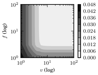
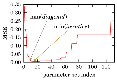
Figure 4: An impact of HO-SVD parameter selection on MSE reconstruction for the Chicken animation. Panel (a) presents the reconstruction error as a function of the number of mode-$1$ ($v$) and mode-$3$ ($f$) components, using the logarithmic scale. Note that the distortion drops sharply with only a few first components. Panel (b) presents the reconstruction error for possible sets of parameters associated with $SS=98.8\%$, obtained by using a method described in 2.6. Annotated sets of best parameters were found by using diagonal and iterative strategies.

Fig. 5 presents $VTF$ ratio for solutions found by using the iterative strategy, as a function of compression ratio. It can be observed that for high $SS$ values, mode-$3$ components, associated with animated frames, tend to be more important than mode-$1$ ones, associated with mesh vertices.

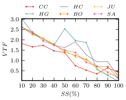
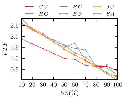
Figure 5: Vertices-to-Frame ratio as a function of $SS$. Experiments were conducted using the best sets of parameters, selected by using the iterative strategy and (a) Hausdorff, (b) MSE metrics.

The distortion introduced by HO-SVD lossy compression, measured with three quality metrics (MSE, Hausdorff, MSDM) is presented in Fig. 6. The method is robust and introduces low distortion even for high compression ratio. Observable deformations for artificial animated meshes (Chicken, Gallop) are almost unnoticeable for $SS\sim 90\%$ and only minor ones are present for $SS\sim 95\%$. For motion capture sequences (Samba, Jumping, Bouncing), major deformations are present for $SS\sim 95\%$, and only minor ones for $SS\sim 85\%$, with unnoticeable distortions for $SS\sim 70\%$. Reconstruction errors are higher for the Collapse mesh, as its animation is hard to describe using rigid transformations. Major deformations are observable for $SS\sim 90\%$, minor ones are present up to $SS\sim 70\%$, and no noticeable distortions for $SS\sim 50\%$ were present. Frames from reconstruction of animations after HO-SVD compression are presented in Fig. 7 (Chicken), Fig. 8 (Collapse) and 9 (Samba). It is worth noting that despite long computation time, MSDM has advantages over other metrics: it is bounded with 1.0 as the maximum value (associated with the worst quality) and it seems to be more sensitive to small, observable distortions of the mesh surface.

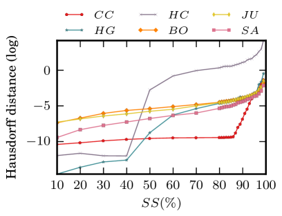
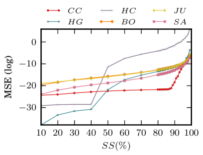
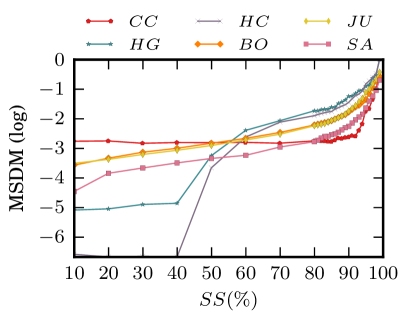
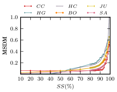
Figure 6: Values of distortion using different 3D quality metrics as a function of $SS$. Panels (a): Hausdorff distance, (b): MSE (c): MSDM are presented in the logarithmic scale. Panel (d) presents the results for the MSDM metric.

A comparison of the reconstruction error occurring when using HO-SVD and PCA is presented in Fig. 10 for Chicken, Gallop, Collapse and Fig. 11 for Samba, Jumping, Bouncing. HO-SVD compression gives better result for a majority of animations. Its advantage is visible especially for motion-capture sequences. Results for Collapse show that both methods have problems with describing non-rigid transformations, and their results are similar for high data compression with HO-SVD introducing lower distortion for low compression.

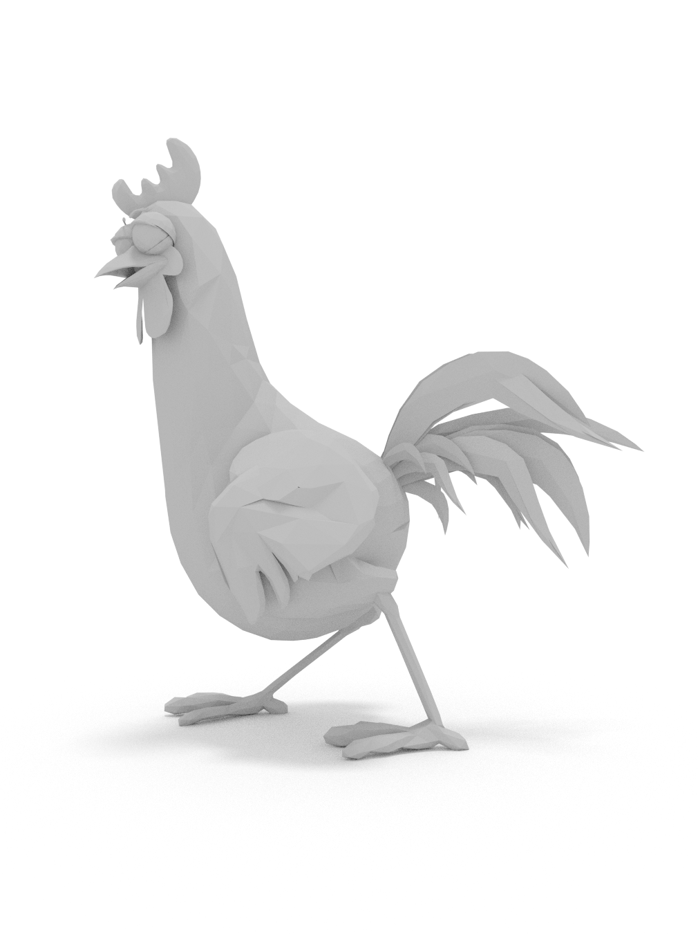
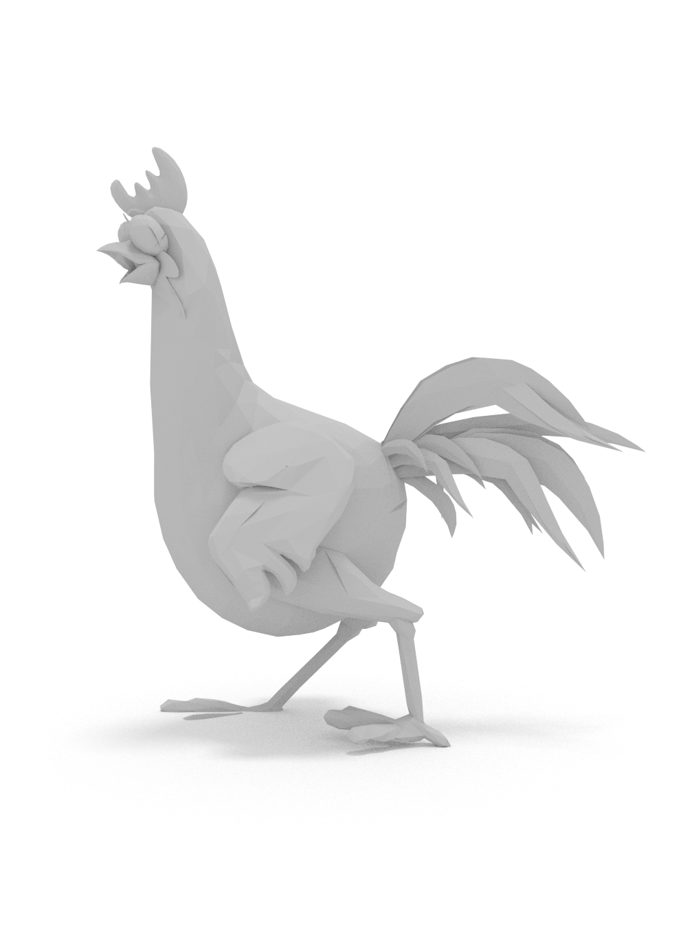
Figure 7: Visualization of a reconstructed model for Chicken. (a): original, (b): SS=94.8%, (c): SS=97.8%, (d): SS=98.8%.

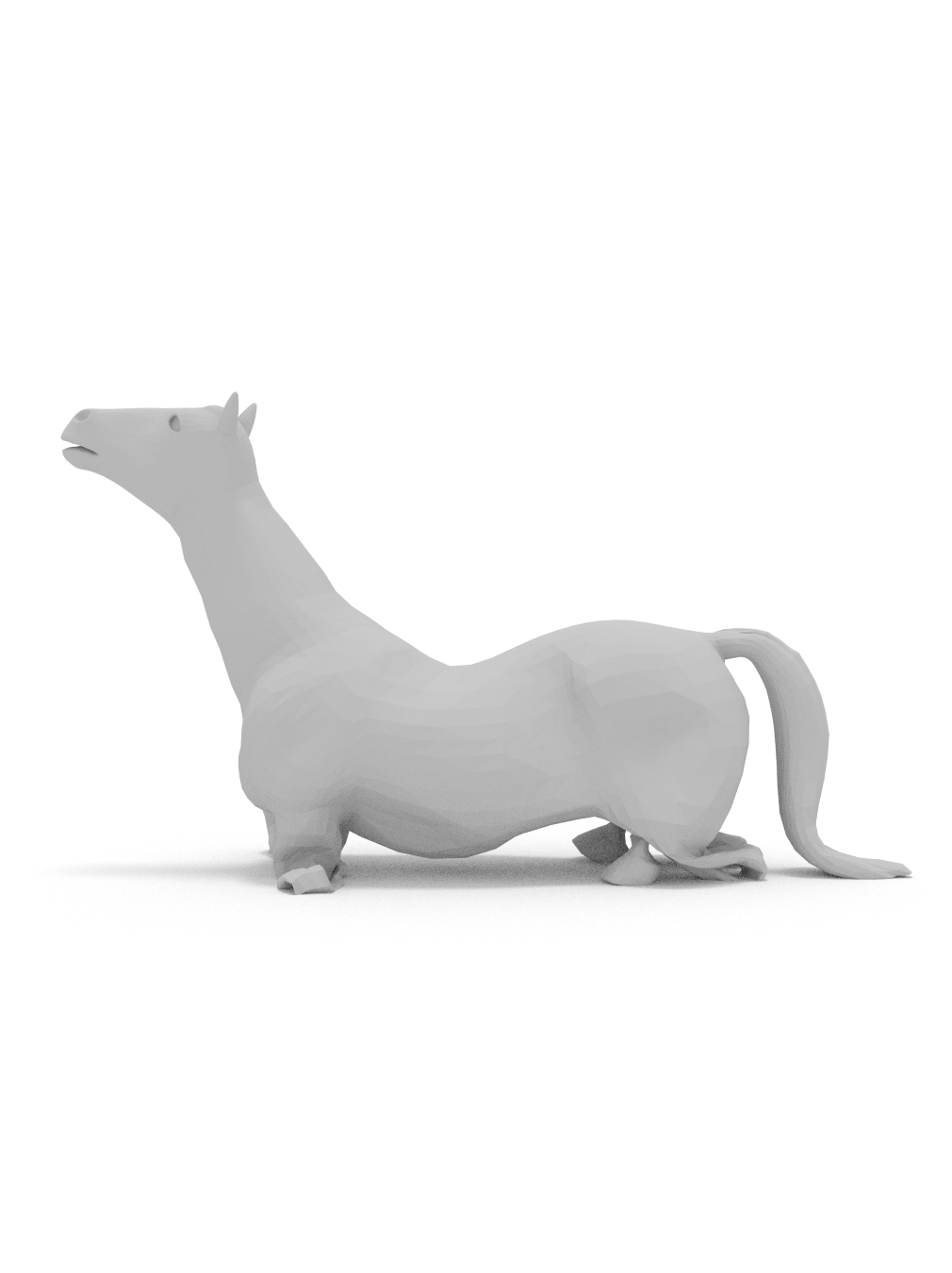
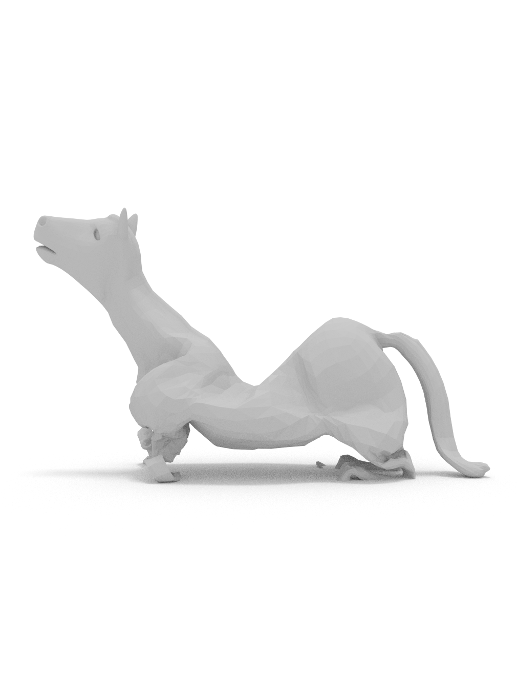
Figure 8: Visualization of a reconstructed model for Collapse. (a): original, (b): SS=69.9%, (c): SS=84.9%, (d): SS=97.9%.

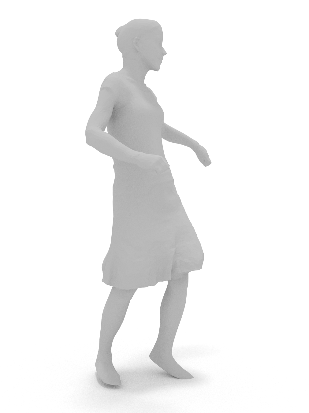
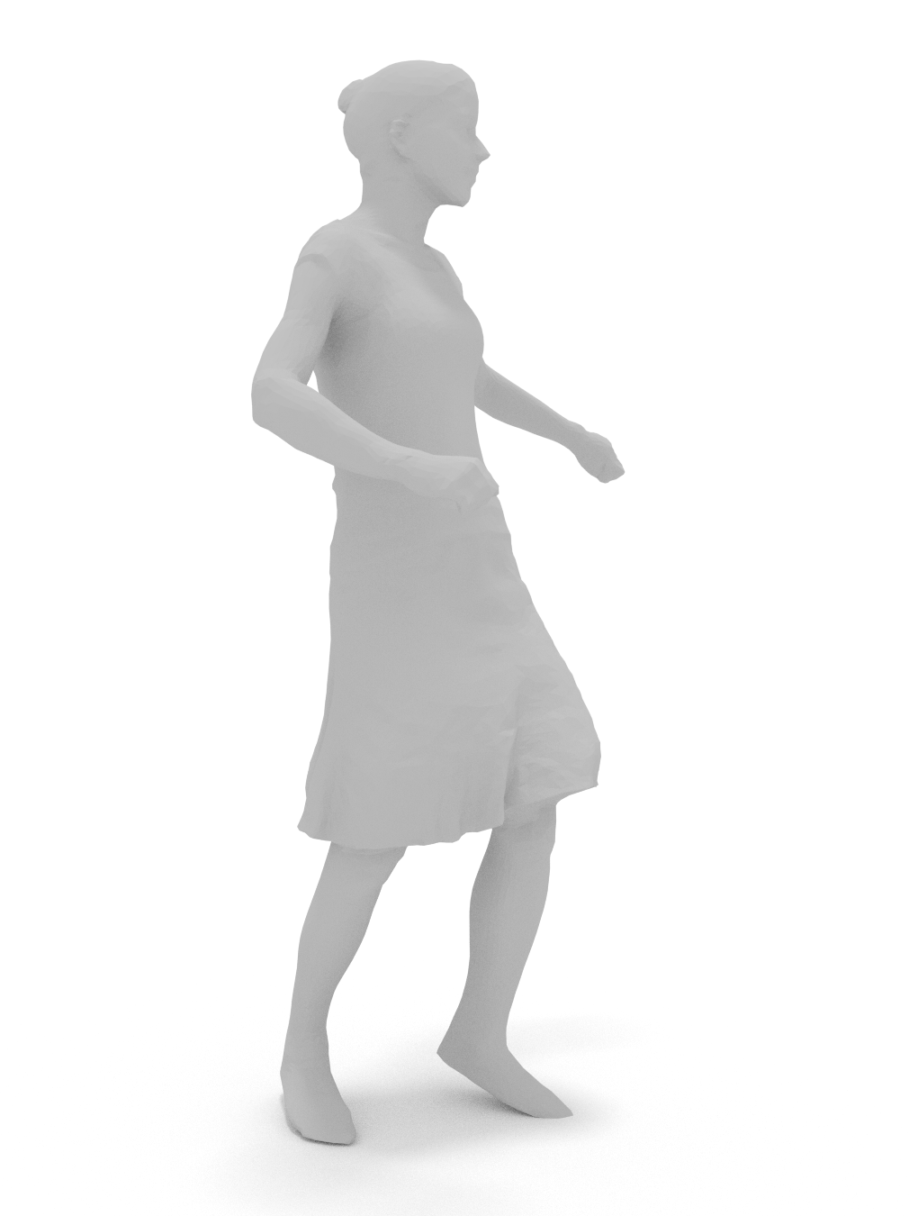
Figure 9: Visualization of a reconstructed model for Samba. (a): original, (b): SS=89.9%, (c): SS=94.9%, (b): SS=97.9%.

4 Conclusions

Our experiments show that HO-SVD allows to achieve good reconstruction quality when applied to compression of 3D animations, and usually outperforms the PCA approach. For most of the animated models and motion-capture sequences, $SS\sim 90\%$ produces a reconstruction similar to the original, especially when lower level-of-detail is required.

The reconstruction error can be measured by using objective metrics, which allows reliable control over compression parameters. For determining the distortion of a reconstructed animation, MSE metric seems to be comparable with the Hausdorff distance while being fast to compute. On the other hand, obtaining MSDM is more time-consuming, but the metric is robust and from our experience it corresponds well with human perception of distortions. Parameters related to the proportion of preserved components in each mode, after performing data decomposition, can be found by using the simple heuristic approach. However, when the speed of coding is critical, the fast strategy for parameter selection is to choose a similar number of components for each mode, which usually produces an acceptable solution.

	Hausdorff	MSDM	MSE
Chicken
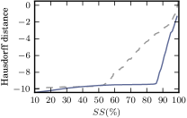
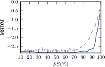
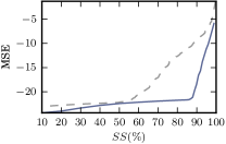
Gallop
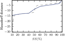
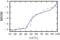
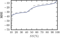
Collapse

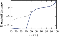
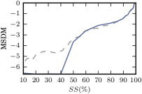
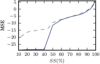
Figure 10: A comparison of HO-SVD (solid line) and PCA (dashed line) reconstruction errors for artificial animations. Distortion is presented in the logarithmic scale as a function of $SS$. Lower values of distortion indicate higher reconstruction quality.

	Hausdorff	MSDM	MSE
Bouncing
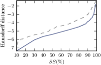
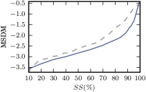
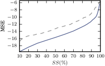
Jumping
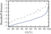
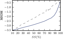
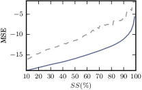
Samba

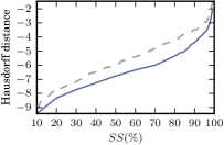
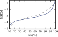
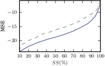
Figure 11: A comparison of HO-SVD (solid line) and PCA (dashed line) reconstruction errors for artificial animations. Distortion is presented in the logarithmic scale as a function of $SS$. Lower values of distortion indicate higher reconstruction quality.

References

- [AM00] Alexa M., Müller W.: Representing Animations by Principal Components. Computer Graphics Forum 19, 3 (2000), 411–418.
- [AS09] Amjoun R., Straíer W.: Single-rate near lossless compression of animated geometry. Comput. Aided Des. 41, 10 (Oct. 2009), 711–718.
- [ASK∗12] Akhter I., Simon T., Khan S., Matthews I., Sheikh Y.: Bilinear spatiotemporal basis models. ACM Transactions on Graphics 31, 2 (Apr. 2012), 17:1–17:12.
- [DLDMV00] De Lathauwer L., De Moor B., Vandewalle J.: A multilinear singular value decomposition. SIAM journal on Matrix Analysis and Applications 21, 4 (2000), 1253–1278.
- [GS13] Głomb P., Sochan A.: Surface Mixture Models for the optimization of object boundary representation. Submitted to International Journal of Computational Geometry and Applications (2013).
- [HPKG08] Huang Y., Peng J., Kuo C.-C., Gopi M.: A Generic Scheme for Progressive Point Cloud Coding. IEEE Transactions on Visualization and Computer Graphics 14, 2 (2008), 440–453.
- [IU05] Inoue K., Urahama K.: DSVD: a tensor-based image compression and recognition method. In Circuits and Systems, 2005. ISCAS 2005. IEEE International Symposium on (2005), pp. 6308–6311 Vol. 6.
- [Jol02] Jolliffe I.: Principal Component Analysis (2nd ed). Springer, 2002.
- [JT05] James D. L., Twigg C. D.: Skinning Mesh Animations. ACM Trans. Graph 24 (2005), 399–407.
- [KB09] Kolda T. G., Bader B. W.: Tensor Decompositions and Applications. SIAM Review 51, 3 (September 2009), 455–500.
- [LDD∗06] Lavoué G., Drelie Gelasca E., Dupont F., Baskurt A., Ebrahimi T.: Perceptually driven 3D distance metrics with application to watermarking. In SPIE Applications of Digital Image Processing XXIX (Aug. 2006).
- [MK07] Mukai T., Kuriyama S.: Multilinear Motion Synthesis with Level-of-Detail Controls. In Computer Graphics and Applications, 2007. PG ‘07. 15th Pacific Conference on (2007), pp. 9–17.
- [MZP08] Mamou K., Zaharia T., Preteux F.: FAMC: The MPEG-4 standard for Animated Mesh Compression. IEEE, Oct 2008, pp. 2676–2679.
- [PKK05] Peng J., Kim C.-S., Kuo C. C. J.: Technologies for 3D mesh compression: A survey. J. Vis. Comun. Image Represent. 16, 6 (Dec. 2005), 688–733.
- [SSK05] Sattler M., Sarlette R., Klein R.: Simple and efficient compression of animation sequences. In Proceedings of the 2005 ACM SIGGRAPH/Eurographics symposium on Computer animation (New York, NY, USA, 2005), SCA ‘05, ACM, pp. 209–217.
- [WA03] Wang H., Ahuja N.: Facial expression decomposition. In Computer Vision, 2003. Proceedings. Ninth IEEE International Conference on (2003), pp. 958–965 vol.2.